Simulations and Effects of Natural Environments on Low Frequency
Antennas with Three-Dimensional FDTD Method
Julien Vincent1, *, Pierre Borderies1, Jean-Ren´e Poirier2, and Vincent Gobin1
Abstract—Three-dimensional Finite-Difference in Time-Domain method is applied to simulate Low
Frequency antennas in the presence of natural environments. All antennas are made up of wires set down on a square shaped ground plane and their dimensions depend on the wavelength of the source. Both monopole and inverted L antennas are considered in this paper. The antenna systems are computed in the presence of two examples of natural elements: a large forest and then on the top of a hill. The main aim of this paper is to show the effects of these environments on the properties of the antennas and on the efficiency of the ground wave excitation. The outcome of these investigations shows a power ratio enhancement of several decibels when the two kinds of antenna described in this paper are located on the top of a hill. On the other hand, the effects of a large forest depend on the geometry of the antenna. It doesn’t affect the radiation of a quarter-wave monopole antenna, on the contrary losses disrupt radiation when an inverted L antenna is built in the middle of a large forest.
1. INTRODUCTION
Low Frequency band (LF) is also known as the kilometer band because the wavelengths λrange from 100 m to 10 km. The radio waves can travel long distance with — at least — three propagation modes: direct (line-of-sight), surface (groundwave) and ionospheric (skywave) modes. Antennas used to transmit information at these frequencies are mainly wire type antennas [1] and the electromagnetic field propagation over usual soils is known [2, 3]. These papers and the references herein deal with the radiation of a dipole over a flat terrain, or over an irregular one at a significant distance from the dipole. As shown in [3], the problem may be split in two steps: the computation of the radiated field at approximately three wavelengths and then the subsequent computation of the propagation with propagation algorithms. For the first step, according to the type of antenna and ground several approaches may be used including full wave ones like integral equation with vertically stratified media [4], which is available in commercial codes. These full wave approaches do not consider to our best knowledge the irregularities of the terrain in the vicinity of the antenna, and however it is well known that such irregularities are influent on the radiation properties since their experimental observations are widely reported, see [5] for example. It is interesting to know how the ground wave reacts when the antenna system is located close to natural elements and how it affects its excitation. The goal of this paper is to treat their 3D modelling.
Finite-Difference in Time-Domain (FDTD) is a well-known method used for computational electromagnetics [6, 7]. The advantages of this technique include a wide frequency range with one single run simulation and conveniences to treat heterogeneous dielectric materials. This method is perfectly adequate here but on the other hand, this scheme requires an upper bound on the time-step, which depends upon space steps to ensure numerical stability and, at low frequencies, we at least have to represent the details of the antenna, leading to small mesh cells. In [8], bi-dimensional FDTD algorithm
Received 7 May 2014, Accepted 10 August 2014, Scheduled 16 August 2014
* Corresponding author: Julien Vincent ([email protected]).
1 Electromagnetism and Radar Department — ONERA, 2 Avenue Edouard Belin, Toulouse 31000, France. 2 Research Group in
is applied to calculate the field strength of Low Frequency (LF) ground wave propagating over irregular terrains. In this paper, three-dimensional FDTD is applied to compute LF wire antennas in the presence of two types of natural environments.
The paper is organized as follows. In Section 2, FDTD method and its principles are described and the formalism of wires is presented. The efficiency of the boundary conditions is then examined and discussed. The geometries of the computed antennas are chosen and all results of the numerical simulations are presented in Section 3. The positions for the antennas are in the middle of a large and high forest and on the top of a hill. In the last part, the conclusions and future prospects are presented.
2. PRINCIPLES OF COMPUTING AND DESIGN OF THE ANTENNAS
In our FDTD code, all wires are implemented with Holland and Simpson formalism [9]. A voltage source can be added on the wire with a time signal known as Rayleigh pulse [10] which presents a null zero-frequency component, helpful for Fourier Transform and frequency domain analysis. The soil of the Earth is considered in this paper as an infinite homogeneous half-plane with relative permittivityεrsand electrical conductivityσs. These parameters depend on the characteristics of the soil and representative values can be found in [11] and reported in Table 1.
Table 1. Dielectric constants and conductivities for different soils.
Earth’s soils εrs σs (S·m−1)
Dry 5 10−4
Medium wet 15 10−3
Wet 30 10−2
Boundary conditions are important parameters in electromagnetic modeling with FDTD. The spatial domain of the computed field is unbounded in real life but it has to be confined for antenna modeling. An absorbing boundary condition is introduced in order to exponentially attenuate the electromagnetic field to reduce reflection. Since they were introduced by Berenger in [12], thePerfectly
Matched Layers (PML) have been extended in many papers [13, 14]. It has been illustrated clearly
in [15] that a strong numerical reflection occurs from the PML of Berenger at low frequencies. Uniaxial-PML (UUniaxial-PML) [16] are then used here to terminate the three-dimensional numerical domain because care should be taken in extending the soil inside the boundary layers. The PML loss parameters are determined by a geometric grading. Firstly, conductivityσ0 at the interface is computed with
σ0 =−
ln(R)·ln(g) 2Z0Δi(gN −1)
(1)
where R is the reflection coefficient, g the scaling factor, Z0 the impedance of free space, Δi the space
step in the PML direction, andN the number of PML cells. Then the PML loss factor is given by the average value in the cell around the index locationL:
σe(0) = σ0·
√g−1
ln(g) (2)
σe(L >0) = σe(0)·gL−1/2 (3)
In this paper, the PML parameters are set to R = 10−4, g = 2 and N = 10 in all computations. Fig. 1 shows the geometry of the problem solved by Sommerfeld [17]: an infinitesimal vertical electric dipole over a dielectric half-space (ε0εrs, μ0, σs) is computed with FDTD and UMPL boundaries. The
electric current element I0l at heighth above the soil transmits to a receiver M at heightz.
At f0 = 100 kHz, with l = 25 m, h = 37.5 m and z = 1 m, propagation of vertical component Ez
ez
eρ eφ
I0l(0, 0, h)
M
(r,0, z)
UPML region
(ε0εrs,μ0,σs)
(ε0,μ0, 0)
→ → →
Figure 1. Geometry of the problem of
Sommerfeld for FDTD computation. The vertical z-directed electric current elementI0lis at height
h above a planar soil with electrical parameters (ε0εrs, μ0, σs). The receiving pointM is at heigth
z and distance r. UPML boundaries terminate the three-dimensional numerical domain.
0 1000 2000 3000 4000 5000 6000 7000 8000 9000 10-5
100 105
Ez (real)
distance (m)
V.m
-1
FDTD FEKO
0 1000 2000 3000 4000 5000 6000 7000 8000 9000 10-5
100 105
Ez (imag)
distance (m)
V.m
-1
FDTD FEKO
Figure 2. Solution comparison of the problem of
Sommerfeld with two different methods, FDTD and MoM computed with the integral solver of F EKO. The vertical electric complex — real and imaginary parts — component Ez with logarithmic scale is computed along the distance r from λ0/10 to 3λ0 at f0 = 100 kHz (300 m to
9 km).
λ
4 −40λ
λ
40
λ
4
(ε0εrs,μ0,σs) (ε0εrs,μ0,σs)
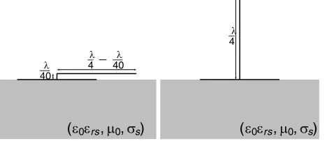
Figure 3. Geometry of the antennas. The inverted L antenna, a small vertical wire (dl=λ0/40) and
a bigger horizontal one (dL=λ0/4−λ0/40), is on the left and the quarter-wave monopole antenna is
on the right. Both antennas are in the middle of a squared ground plane (width =λ0/4).
modeling of the soil for our distance of interest: fromλ0/10 to 3λ0. Remotely from this distance, one can
use propagation techniques of DeMinco [3]. More complex natural environments can be implemented in the FDTD model which is done in the following.
3. RESULTS AND DISCUSSIONS
The simulated antennas are an inverted L antenna and a quarter-wave monopole antennas at the frequencyf0 = 100 kHz. They are both made up of two parts: a wire and a square shaped ground, as
shown in Fig. 3. We shall now introduce the examples of natural environments.
3.1. Large Forest
According to [18], a forest can be represented by a dielectric slab with corresponding dielectric constant εrf and σf for this range of frequency. The values (εrf = 1.065;σf = 10−3S·m−1) are used here for a
3.1.1. Inverted L Antenna
At the frequency f0 = 100 kHz, an inverted L antenna is located at the center of a square shaped
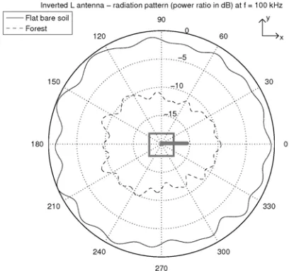
(width = 12 km, height = 25 m) forest. Fig. 4 and Fig. 5 show the results of the simulations. On the first one the squared magnitude of the electric field |E|2 is sampled at 9 km around the antenna, 1 m over the ground and then normalized by the input power. In Fig. 5 the power ratio in dB is sampled along the y direction of propagation, 1 m over the ground.
One can observe in Fig. 4 that the shape of the radiation pattern does not change when this type of antenna is placed in the forest. Nevertheless a 10 dB loss occurs with the natural element. The modelling in Fig. 5 shows that the signal partially recovers itself beyond the forest at 6 km. This effect is similar to the Millington recovery effect [19]. However due to losses inside the dielectric slab, the power density at the end of the forest is smaller than the power density obtained with the flat bare soil case.
Figure 4. Simulations of an inverted
L antenna at f = 100 kHz with and without the large forest. The antenna is drawn in the middle, according to the axes orientation the horizontal wire is along x
direction.
1000 2000 3000 4000 5000 6000 7000 8000 9000 -50
-40 -30 -20 -10 0
distance (m)
|E|
2/P
in
(dB)
Inverted L antenna - Propagation of electric field along y direction
Flat bare soil Forest
Figure 5. Simulations of an inverted L antenna at
f = 100 kHz with and without the large forest along
y direction from 1.2 km to 9 km. With the environment a recovery effect known as Millington effect is observed at the end of the forest (6 km).
3.1.2. Quarter-Wave Monopole Antenna
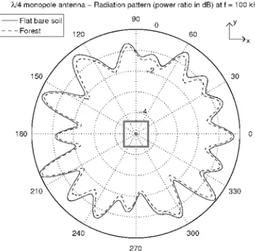
The same methodology was applied to a quarter-wave monopole antenna emitting at f0 = 100 kHz. It
was computed in the presence of the forest described in the previous section. The squared magnitude of the electric field|E|2at 9 km around the antenna and 1 m over the ground is normalized by the input power.
As shown in Fig. 6 the radiation patterns are similar, one deduces that the forest do not interfere with this type of antenna. This is quite logical because only a small part of the antenna is inside the forest in this (rather theoretical) case. This is confirmed with the results in Fig. 7. The power ratio is lower in the forest from 0 to 6 km and it completely recovers itself a little further.
Figure 6. Simulations of a quarter-wave monopole antenna with and without the forest. At f0 = 100 kHz, the antenna is
built in the middle of the system and the results are sampled at 9 km around it and normalized by the input power.
1000 2000 3000 4000 5000 6000 7000 8000 9000 -35
-30 -25 -20 -15 -10 -5 0
Inverted L antenna − Propagation of electric field along y direction
distance (m)
|E|
2/P
in
(dB)
Flat bare soil Forest
Figure 7. Simulations of a quarter-wave monopole
antenna atf = 100 kHz with and without the forest along
y direction from 1.2 km to 9 km.
soil is modified by the presence of the forest. This frequency change is taken into account by the input power normalization. Secondly one can observe power losses presumably due to the natural element wich absorbs a part of the energy emitted by this antenna.
3.2. On the Top of a Hill
The cartesian grid of the FDTD method requires the use of multiple dielectric blocks defined by (εrh; σh). They are created with different sizes in order to build a hill with an average slope, see Fig. 8. The hill and the soil have the same dielectric constants (εrh=εrs; σh =σs).
(ε0εrs,μ0,σs)
(ε0,μ0, 0)
Figure 8. Hill created for FDTD simulations, in this case: four 25 m height dielectric slabs are stacked
on each other, their widths are chosen in order to create an average eleven percent slope. The height of antennas equals three times of the height of a dielectric slab. The antenna is located on the top of the hill.
3.2.1. Inverted L Antenna
An inverted L antenna at the frequencyf0= 100 kHz is located on the top of a hill made up of 4 square
shaped dielectric blocks. All of them are 25 m high and their width are calculated so as to create an eleven percent average slope.
The interactions with two different soils — dry (εrs = 5; σs = 10−4S·m−1) and medium
Figure 9. Simulations of an inverted L antenna at f = 100 kHz with and without the hill on dry soil (εrs = 5; σs = 10−4S·m−1). The squared magnitude of the electric field is sampled at 9 km around the antenna and 1 m over the ground and normalized by the input power.
1000 2000 3000 4000 5000 6000 7000 8000 9000 -25
-20 -15 -10 -5 0
Inverted L antenna − Power ratio in dB along y direction
distance (m)
|E|
2/P
in
(dB)
Flat bare soil Hill
Figure 10. Simulations of an inverted L antenna with
and without the hill on dry (εrs= 5; σs= 10−4S·m−1) soil along y direction.
Figure 11. Simulations of an inverted L
antenna at f = 100 kHz with and without the hill on medium wet (εrs = 15; σs = 10−3S·m−1) soil. The squared magnitude of the electric field is sampled at 9 km around the antenna and 1 m over the ground and normalized by the input power.
1000 2000 3000 4000 5000 6000 7000 8000 9000 -25
-20 -15 -10 -5 0
Inverted L antenna − Power ratio in dB along y direction
distance (m)
|E|
2/P
in
(dB)
Flat bare soil Hill
Figure 12. Simulations of an inverted L antenna at
f = 100 kHz with and without the hill on medium wet (εrs= 15; σs= 10−3S·m−1) soil along y direction.
Now the power ratio in dB is computed along y direction of propagation in Fig. 10 and Fig. 12. The values are sampled from 1.5 km to 9 km and 1 m over the soil far from the antenna and the end of the hill. One can see on these figures that the system is more efficient when it is located on the top of a hill, the gain of efficiency increasing with the wetness: 3 dB with on a dry soil and 6 dB on a medium wet soil.
3.2.2. Quarter-Wave Monopole Antenna
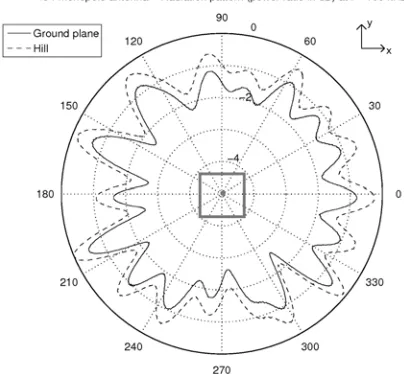
The inverted L antenna is replaced by a quarter-wave monopole antenna on a medium soil. The outputs shown in Fig. 13 and Fig. 14 are the same as the previous section. In all directions and on all distances of observation, the power ratio is upper of a few dB when the quarter-wave monopole antenna is built on the top of a hill, but of a much smaller amount.
Figure 13. Simulations of a quarter-wave
monopole antenna at f = 100 kHz with and without the hill on medium wet (εrs = 15; σs = 10−3S·m−1) soil. The squared
magnitude of the electric field is sampled at 9 km around the antenna and 1 m over the ground and normalized by the input power.
1000 2000 3000 4000 5000 6000 7000 8000 9000
-15 -10 -5 0
distance (m)
|E|
2/P
in
(dB)
λ/4 monopole antenna − Power ratio in dB along y direction
Flat bare soil Hill
Figure 14. Simulations of a quarter-wave monopole
antenna at f = 100 kHz with and without the hill on medium wet (εrs = 15; σs = 10−3S·m−1) soil along y
direction.
4. CONCLUSIONS
REFERENCES
1. Rudge, A. W., K. Milne, A. D. Olver, and K. Knight, The Handbook of Antenna Design Volumes
1 and 2, Peter Peregrinus Ltd, London, 1986.
2. Maclean, T. S. M. and Z. Wu, Radiowave Propagation Over Ground, Chapman & Hall, London, 1993.
3. DeMinco, N., “Propagation prediction techniques and antenna modeling (150 to 1705 kHz) for intelligent transportation systems (ITS) broadcast applications,”IEEE Antennas and Propagation
Magazine, Vol. 42, No. 4, 9–34, August 2000.
4. Tsang, L., C.-C. Huang, and C. H., Chan, “Surface electric fields and impedance matrix elements of stratified media,”IEEE Transactions on Antennas and Propagation, Vol. 48, No. 10, 1533–1543, October 2000.
5. Belrose, J. S., W. L. Hatton, C. A. McKerrow, and R. S. Thain, “The engineering of communication systems for low radio frequencies,” Proceeding of the IRE, Vol. 47, No. 5, 661–680, May 1959. 6. Yee, K. S., “Numerical solution of initial boundary value problems involving Maxwell’s equations
in isotropic media,” IEEE Transactions on Antennas and Propagation, Vol. 14, No. 3, 302–307, May 1966.
7. Taflove, A. and S. C. Hagness,The Finite-Difference Time Domain Method, Artech House, London, 2005.
8. Zhou, L., X. Xi, J. Liu, and N. Yu, “LF ground-wave propagation over irregular terrain,” IEEE
Transactions on Antennas and Propagation, Vol. 59, No. 4, 1254–1260, April 2011.
9. Holland, R. and L. Simpson, “Finite-difference analysis of EMP coupling to thin struts and wires,”
IEEE Transactions on Electromagnetic Compatibility, Vol. 23, No. 2, 88–97, May 1981.
10. Hubral, P. and M. Tygel, “Analysis of the Rayleigh pulse,” Geophysics, Vol. 54, No. 5, 654–658, May 1989.
11. Von Hippel, A. R., Dielectric Materials and Applications, M.I.T. Press, Cambridge, 1954.
12. Berenger, J. P., “A Perfectly Matched Layer for the absorption of electromagnetic waves,” J.
Computational Physics, Vol. 114, 185–200, 1994.
13. Chew, W. C. and W. H. Weedon, “A 3D perfectly matched medium from modified Maxwell’s equations with stretched coordinates,”IEEE Microwave Guided Wave Lett., Vol. 7, 599–604, 1994. 14. Roden, J. A. and S. D. Gedney, “Convolutional PML (CPML): An efficient FDTD implementation
of the CFS-PML for arbitrary media,”Microwave Optical Tech. Lett., Vol. 27, 334–339, 2000. 15. De Moerloose, J. and M. A. Stuchly, “Behavior of Berenger’s ABC for evanescent waves,” IEEE
Microwave and Guided Wave Letters, Vol. 5, No. 10, 344–346, October 1995.
16. Gedney, S. D., “An anisotropic Perfectly Matched Layer absorbing medium for the truncation of FDTD lattices,” IEEE Transactions on Antennas and Propagation, Vol. 44, No. 12, 1630–1639, December 1996.
17. Sommerfeld, A., “Propagation of waves in wireless telegraphy,”Annalen der Physik, Vol. 28, 665– 736, March 1909.
18. Tewari, R. K., S. Swarup, and M. N. Roy, “Evaluation of relative permittivity and conductivity of forest slab from experimental measured data on lateral wave attenuation constant,” International
Journal of Electronics, Vol. 61, 597–605, November 1986.