Inverse Wave Scattering of Rough Surfaces with Emitters
and Receivers in the Transition Zone
Slimane Arhab1, * and Gabriel Soriano2
Abstract—We deal with the problem of determining the profile of a perfectly conducting rough surface
from single-frequency and multistatic data. The two fundamental polarizations are investigated, in a two-dimension scattering configuration. Emitting and receiving antennas are positioned on a probing line some wavelengths above the profile. It is shown how the boundary integral equation method can be adapted to the case where the antenna footprint is much wider that the rough part of the profile. The Newton-Kantorovich iterative inversion process is then performed on these synthetic data. Its accuracy and robustness to additive noise are studied in the context of random rough surfaces with correlation length smaller than the wavelength and slope root mean square up to 0.9.
1. INTRODUCTION
The problem of determining the roughness of a surface from scattering data is encountered in many applications in both microwave and optical domains. The microwave remote sensing of natural surfaces such as sea, sand, soils or snow [1] is a major topic in geoscience. The scattered field from a rough soil can also hinder the detection, localization and characterization of some buried objects. Optical profilers provide through several chromatic or interferometric technologies non-contact surface metrology for design characterization and process control [2].
Methods were developed to deal with the difficulties associated to this class of inverse problem [3], namely non-linearity and ill-posedness [4]. Most common approaches consider approximate surface scattering theories [5] for describing the interaction between the electromagnetic field and the roughness. Those single scattering approximations are of theoretical and practical importance, since they can often be inversed analytically. In the early nineties were published inversion schemes based on the small perturbation method [6–8], the Kirchhoff approximation [9, 10] and the Rytov approximation [11]. More recently, a scattered field correlation procedure was developed in the framework of the small perturbation theory to characterize both the surface roughness and buried objects [12]. Each method has its own validity domain [13], but they are all restricted to configurations (roughness, angles) where multiple scattering is negligible.
For the scattering from a rough surface, the boundary integral equation method [14, 15] is the most fitted and commonly used numerical solution of the rigorous direct scattering problem, since it requires only the surface to be sampled. This method was efficiently implemented in inverse scattering schemes for two-dimensional [6, 16, 17] and three-dimensional [18] scattering. However, one requisite of the method is that the incident field is a tapered wave, usually a gaussian beam. This is a way to avoid the unphysical scattering from the edges of the sampled surface. In this paper, another approach is followed [19], where the rough surface is a local deformation of a plane. Stability and convergence of this finite section method when the roughness becomes non-local was studied in [20]. A classical configuration
Received 30 October 2015, Accepted 15 December 2015, Scheduled 2 January 2016 * Corresponding author: Slimane Arhab ([email protected]).
1 Universit´e d’Avignon et des Pays de Vaucluse, UMR 1114 EMMAH, Avignon Cedex 84018, France. 2 Aix-Marseille Universit´e,
in microwaves is addressed where a set of antennas positioned on a horizontal line successively illuminate the rough surface that stands some wavelengths below. On one hand, the antennas are too distant from the surface for evanescent waves to rule the interaction, as in near-field. On the other hand, that distance is too short for far-field regime to be reached. The antennas are in the transition or intermediate zone. The forward model is presented in Section 2 for both fundamental polarization cases. The paper is restricted to two-dimensional scattering and perfectly conducting profiles.
The inverse problem is solved iteratively with the Newton-Kantorovich method [21, 22]. To constitute the data set, emitters also function as receivers. The profile cannot be estimated directly from that data set. The inverse problem is thus recasted as an optimization problem. The solution is built up iteratively by successively solving the forward problem and a local linear inverse problem. With the locally rough plane approach, the forward problem can be accurately modelized despite the fact that the emitters footprints on the profile are much wider than the sampled part of the profile. The local linear inverse problem relies on the calculus of the Fr´echet derivative of the non-linear scattering operator. Based on the reciprocity theorem, this calculus was first proposed in far-field configuration [23]. It is here adapted to localized emitters and receivers. The inverse problem is detailed in Section 3.
This inversion scheme is tested on synthetic data. Realizations of Gaussian random rough profiles with varied correlation length are reconstructed, starting from the undeformed plane. Influence of polarization is underlined. Note that unusually rough surfaces are investigated in this paper, with the will to push the method to its limits. Section 4 is devoted to these numerical results. The paper is concluded in Section 5.
2. FORWARD PROBLEM
2.1. Configuration of the Study
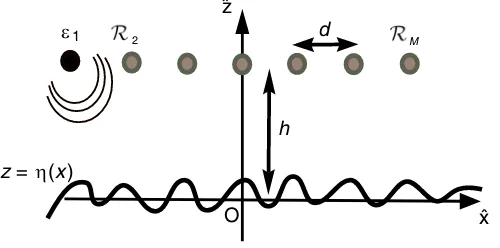
In a Cartesian coordinates system (O, x, y, z) the rough surface Γ is invariant along the Oy axis (see Figure 1). Its profile is described by the equation z =η(x). The function η is twice differentiable and non-zero only for |x| ≤ T/2. The unit vector ˆn normal to the surface is directed toward the air. The field of study is the y-component of the electric field in the TE case (E = ψte(x, z) ˆy), while it is the
y-component of the magnetic field in the TM case (H=ψtm(x, z) ˆy). We assume a time dependence e−iωt at a fixed angular frequencyω.
O ˆx
ˆz
z=η (x)
ε1 2 M
h d
Figure 1. Geometry of the problem.
2.2. Incident Field
Let us now consider a set of M antennas located along a horizontal line with an interdistance d, at a height h from the average plane z = 0 of the surface. Each one of them plays the role of emitter and receiver but not simultaneously. When an antenna l acts like an emitter E, l ∈ {1,2, . . . ,M}
For the TE polarization, an emitter E located at r = xxˆ + zˆz is set to produce an incident electric field on the pointr = xˆx +zˆz of space:
Einc =ψi,te(r) ˆy=−
1 4ωμo H
(1)
0 (k|r − r|) ˆy (1)
in order to mimic an electric dipole with moment oriented along the invariance direction ˆyof the surface. H(1)0 is the first-kind Hankel function of zero-order whilekdenotes the wavenumber in the air at angular frequencyω.
Rotating the electric dipole of the emitterE of a quarter turn in the (xOy) plane gives an electric dipole moment along ˆx, that is associated to an illumination under the TM polarization:
Hinc =ψi,tm(r) ˆy=−
i k 4 H
(1)
1 (k|r − r|)
z−z
|r − r|yˆ (2)
with H(1)1 the first-kind Hankel function of first-order.
2.3. Boundary Integral Formalism
Since the surface is a local deformation of the horizontal plane, the total field ψ writes as the sum of the incident field ψi as defined previously and the field ψr that would be reflected by the horizontal
plane according to the boundary conditions and the scattered fieldψs that represents the contribution of the roughness.
ψ =ψi +ψr+ψs (3)
This scattered fieldψs, that satisfies a radiation condition in the air, has a Kirchhoff-Helmholtz integral
representation in this half-space: for an observation pointr=xxˆ+zˆz outside Γ,
Γ
∂ng(r,r)ψs(r) −g(r,r)∂nψs(r)
dΓ =
ψs(r) z > η(x)
0 z < η(x) (4)
with r =xxˆ+η(x)ˆz the integration point over Γ, or source point. The scattered fieldψs(r) and its
normal derivative ∂nψs(r) are taken at the limit from the air onto the surface. The free space Green’s
function in the air is g(r,r) = 4iH0(1)(k|r−r|), and ∂ng(r,r) = ˆn(r)· ∇rg(r,r) denotes its normal
derivative with respect to the source point.
At the limit when the observation point r tends toward the profile, from air or from the metal, formula (4) leads to the integral equation:
1 2ψ
s(r)−
Γ
∂ng(r,r)ψs(r)dΓ +
Γ
g(r,r)∂nψs(r)dΓ = 0 (5)
where bothrandrare points on the profile Γ. With two independant unknown surface densitiesψsand
∂nψs, Equation (5) can only be solved with a supplementary equation, that is the boundary condition
on the profile. Depending on the polarization case,
ψte = 0 = ψi,te+ψr,te+ψs,te (6)
∂nψtm = 0 = ∂nψi,tm+∂nψr,tm+∂nψs,tm (7)
on any point of the profile Γ.
Therefore, the forward problem can be solved by means of two coupled equations. The first one, denoted as observation equation, relates the scattered field measured on the receivers to the unknown surface density. This unknwon is obtained by solving the second equation, the so-called state equation, for a given profile-function and a well known incident field. We now summarize the two different polarization cases. Under the TE polarization, where the surface unknown is given by the normal derivative of the scattered field on the rough surface∂nψte, the observation Equation (8) and the state
Equation (9) write:
ψtem =ψim,te+ψrm,te−
Γ
g(rm,r)∂nψs,te(r) dΓ−
Γ
∂ng(rm,r) (ψi,te(r) +ψr,te(r)) dΓ (8)
Γ
g(r,r)∂nψs,te(r)dΓ =
1 2(ψ
i,te(r) +ψr,te(r))−
Γ
In TE polarization, receivers are sensitive to the total fieldψtem=ψte (rm), while it is the derivative with respect to the z variable ∂zψtmm = ∂zψtm (rm) in TM polarization, since measurement is proportional to the total electric field component along the receiver electric dipole moment. Therefore, the forward model in the TM case is
∂zψmtm=∂zψim,tm+∂zψmr,tm+
Γ
∂zg(rm,r)(∂nψi,tm(r)+∂nψr,tm(r))dΓ+
Γ
∂z∂ng(rm,r)ψs,tm(r) dΓ (10)
1 2ψ
s,tm(r)−
Γ
∂ng(r,r)ψs,tm(r)dΓ =
Γ
g(r,r)(∂nψi,tm(r) +∂nψr,tm(r))dΓ (11)
For both polarizations, the data setU (U ={ψtem}m, orU ={∂zψtmm}m,) is related to the profile-functionη via a non-linear operator Finvolving the coupled equations of fields reported in (8) and (9) for TE polarization and in (10) and (11) for TM polarization:
η→ U =Fη (12)
Full details about the numerical implementation of these equations can be found in the reference [14]. To solve the inverse problem of determining the profile function from the scattered field data, a naive approach is to try finding the inverse operator F−1. In practice however, such a direct approach proves impossible because of forward operator Fnon-linearity.
3. INVERSE PROBLEM
3.1. Fr´echet Derivative of the Scattering Operator
To solve this inverse problem, Newton-Kantorovich linearization is considered. This is done by finding
D the Fr´echet derivative ofFat η involved in the linear relationship:
F(η+δη) =Fη+Dδη+ o(δη2), as δη2 →0
F(η+δη)−Fη =δU Dδη, (13)
Here, δη symbolizes a small variation of the profile-function and δU the linked small variation of the scattered field. The expression of the linear operator D can be deduced from the reciprocity theorem. In [23], it was introduced in far-field configuration with an illumination by plane waves. In this work, we adapt this approach to emission of the incident field and reception of the total field by electric dipoles, localized in the transition zone, and for a perfectly conducting rough surface. With an invariance axis, the Fr´echet operatorD takes the following forms
δUte =Dteδη δψtem = −i
ωμo
Γ
∂nψ(r)∂nψm(r)δη(r) dΓ (14)
in TE polarization, while in the TM case,
δUtm =Dtmδη δ∂zψsm =
Γ
{∂tψ(r)∂tψm(r)−k2ψ(r)ψm(r)}δη(r) dΓ (15)
3.2. Iterative Process
It is now possible to estimate the actual profile-functionηa of a rough surface for which we measure the
dataUmes, by building an iterative process of updating the profile at each stepn:
ηn=ηn−1+δηn (16)
The correctionδηn is obtained by minimizing the cost functionalξ. It expresses in the sense ofL2 norm
the error (δU −Dδη) of the linear system of equations (Equation (13)). Therefore, we have: ⎧
⎪ ⎨ ⎪ ⎩
ξ(δη) =(Umes − Un−1)−Dn−1δη2 2
minξ(δη)⇔δη =δηn
With:δηn= [D†n−1Dn−1]−1D†n−1(Umes− Un−1)
The † symbol stands for the transposed complex conjugation. Un−1 in Equation (18) denotes the data
associated to the best available estimation of the profile-functionηn−1computed thanks to Equations (8)
and (9) in TE polarization and to Equations (10) and (11) in TM polarization. Unfortunately, the solution δηn obtained at this stage is unstable. The inverse problem remains ill-posed because the
continuity of the solution against data is not satisfied. Numerically, the consequence is an ill-conditioned matrixD†n−1Dn−1. Noise due to model errors is thus amplified in the data (Umes− Un−1). This leads
to grossly erroneous estimation ofδηn. To overcome this difficulty, we introduce a mixture of zero and
second order standard Tikhonov regularization [4]. The cost functional is thus changed fromξ to ˜ξ: ⎧
⎪ ⎨ ⎪ ⎩
˜
ξ(δη) =(Umes− Un−1)−D
n−1δη22 + μ2(αSδη22 + (1−α)Iδη22)
min ˜ξ(δη)⇔δη=δη˜n
δη˜n= [D†n−1Dn−1 + μ2(αS†S+ (1−α)I)]−1D†n−1(Umes− Un−1),
(18)
I being the identity operator. S stands for the second-order derivative operator such as S[δη] =
d2
dx2[δη(x)]. Both regularization terms serve to stabilize the solution by adding a constraint on the
profile height and curvature, each weighted by the mixing parameter α. Note that the regularization parameterμ2 does not vary during the iterative process and its value is chosen by trial and error.
3.3. The First-Order Small Perturbation Method
The small perturbation method is the oldest and perhaps most popular method in wave scattering from rough surfaces. It is a perturbative expansion of the field scattered from a rough surface with respect to a small height over wavelength ratio. Derivation of that method for a one-dimensional perfectly conducting surface can be found up to the second order in many classical textbooks such as [24]. In such a classical derivation, incident field is a plane wave, while scattered field is approximated in the far-field regime. It is remarkable that Equations (14) and (15), when applied to a flat profile η = 0, form expressions of the first-order small perturbation method (SPM1) generalized to arbitrary incident and scattered fields.
Since the iterative process described in paragraph 3.2 is precisely started at first stepn= 1 from the horizontal planeη0 = 0, the profile variationδη1, solution of the linear problem (18), can be considered
as a regularized inverse ηSP M1 of the SPM1 approximate scattering theory. This profile ηSP M1 =δη1
will be used in the Section 4 on numerical results as a representative of the approximate methods.
4. NUMERICAL RESULTS ON SYNTHETIC DATA
Synthetic data are generated with the forward model presented in Section 2. The number of points to describe the actual profile is Nr = 5280. To avoid as much as possible an inverse crime, the profile estimated at each iteration is discretized with a different number of points N = 2640. Note that this amount of data is much smaller than the number of points on the profile.
The emitters wavelength in the air is denotedλ, and is used as the length unit in the whole section. The number of emitters/receivers used is M= 21. It consists in a set of electric dipoles located along a horizontal line piece with an interdistance d = 2.4λ, at a height h = 4λ from the average plane of the surface. Backscattering is disregarded, since the dipole cannot act simultaneously as an emitter and as a receiver. Therefore, the total number of redundancy-free scattered field data is equal to (M −1)M/2 = 210.
The studied surfaces are realizations of a Gaussian random process with Gaussian spectrum [14]. The roughness is thus characterized by two statistical parameters, the height root mean square hrms
and the correlation length lcor. For such a spectrum, the profile slope root mean square is simply given by srms =√2hrms/lcor. First, we set their root mean square height hrms = 0.095λ and we vary the correlation length in the range lcor ∈ [0.15; 0.5]λ. Second, the correlation length is fixed to
T = 48λ. This flattening aims at suppressing numerical artefacts due to edge effects (see Sections 2 and [19]).
To monitor the iterative process, we introduced two convergence criteria, namely REFnthe residual
error field and REPn the residual error profile. They are both calculated in the sense ofL2 norm. The
first is defined as the difference between the simulated data and the measured field, while the second gives the difference between the estimated profile and the actual profile:
REFn=Umes− Un22/Umes22 REPn=ηa−ηn22/ηa||22 (19)
The main objective here is to test the ability of the algorithm to reconstruct the surface roughness by processing the data. We proceed in three different ways. First and second, a single-polaization data set is processed, that is TE or TM, respectively. Third, the profile is estimated from dual-polarized data, that is by processing simultaneously the TE and TM data sets.
In the TE-only and TM-only cases, the solution is obtained by minimizing the cost functional (Equation (18)), starting from thez= 0 horizontal plane as the profile initial guess. For the TE data, we note that the residual error between the actual profile and the reconstructed profile (Figure 2(a)) increases continuously with decreasing correlation length.
For the TM data, we observe (Figure 2(a)) a same continuous behaviour until the correlation length reaches the value lcor= 0.4λ. At this point, the residual error increases suddenly giving an incorrect estimation of the profile.
lcor [wavelength]
0.15 0.2
0.25 0.3
0.35 0.4
0.45 0.5
Residual Error Profile [%]
0 20 40 60 80 100
REP (last iteration step) based on TE data REP (last iteration step) based on TM data REP (last iteration step) based on TE-TM data
lcor [wavelength]
0.15 0.2
0.25 0.3
0.35 0.4
0.45 0.5
Residual Error Profile [%]
0 5 10 15 20 25 30 35
REP (last iteration step) based on TE data
REP (last iteration step) based on TE-TM data (a)
(b)
Figure 2. The last iteration step residual error profile as a function of the profile correlation length
In order to process TE and TM data together, we introduce a new weighting parameter ν in the cost functional:⎧
⎪ ⎪ ⎪ ⎪ ⎪ ⎪ ⎪ ⎨ ⎪ ⎪ ⎪ ⎪ ⎪ ⎪ ⎪ ⎩
˜
ξ∗(δη) =(Utemes − Uten−1)−Dte,n−1δη22+ν2(Utmmes− Utmn−1)−Dtm,n−1δη22
+μ2(αSδη2
2 + (1−α)Iδη22)
min ˜ξ∗(δη)⇔δη =δη˜∗n
δη˜n∗ = [D†te,n−1Dte,n−1+ν2D†tm,n−1Dtm,n−1 +μ2(αS†S+ (1−α)I)]−1
(D†te,n−1(Utemes− Uten−1) + ν2D†tm,n−1(Utmmes− Utmn−1) )
(20)
With ν2 = 10−3, the TM data weight is lowered in the algorithm, so that the reconstructed profile for short correlation lengths (Figure 2(b)) gets improved. Evolution of the residual error profile at short correlation length lcor= 0.2λagainst the varying height root mean square is plotted in Figure 3. As usual, the z = 0 plane is used as initial guess. For a profile which has a correlation length equal to
lcor = 0.2λ, the behaviour of the two objective criteria (REFn, REPn) during the iterative process
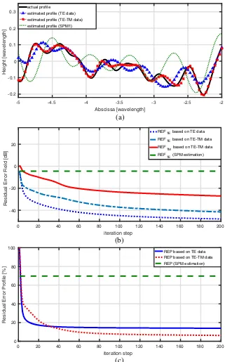
(Figures 4(b) and 4(c)), shows a significant improvement compared to the TE data inversion. Indeed, the depth of some hollows is poorly estimated with the first set of data (TE data), while a simultaneous use of all the data sets (TE-TM data), allows a reconstruction of almost all the hollows of the roughness and the finest details of the surface (Figures 4(a) and 4(b)). For both residual errors REF and REP, plots in Figures 4(b) and 4(c) clearly indicate that the first iteration solution (SPM1) is a very coarse estimation of the profile. Here, the SPM1 residual error profile reaches 70%. For this error to be reduced, the first dozen iterations appear particularly profitable.
hrms [wavelength]
0.08 0.09 0.1 0.11 0.12 0.13 0.14
Residual Error Profile [%]
0 5 10 15 20 25
REP (last iteration step) based on TE-TM data
Figure 3. The last iteration step residual error profile as a function of the profile height root mean
square hrms,∈ [0.08λ; 0.14λ] for a correlation length lcor= 0.2λ: inversions of the combined TE-TM data sets.
To summarize those results on noiseless synthetic data, the residual error profile after one hundred iterations remains smaller than 2.5% for correlation length larger than 0.3λ(RMS slope smaller than 0.45), and smaller than 10% for correlation length larger than 0.18λ (RMS slope smaller than 0.75). These outstanding performances are obtained with our iterative process applied on dual-polarized data. Note that an inversion process of data under both polarizations takes around one hour run time for one hundred iterations. These simulations were performed using MATLAB with no particular optimizations on a personal computer, with a dual-core processor at 2.67 GHz and 4 Gb central memory.
Abscissa [wavelength]
-5 -4.5 -4 -3.5 -3 -2.5 -2
Height [wavelength]
-0.2 -0.1 0 0.1 0.2 0.3
actual profile
estimated profile (TE data) estimated profile (TE-TM data) estimated profile (SPM1)
(a)
iteration step
0 20 40 60 80 100 120 140 160 180 200
Residual Error Field [dB]
-40 -20 0 20
REFTE based on TE data REF
TE based on TE-TM data
REF
TM based on TE-TM data
REFTE (SPM estimation)
iteration step
0 20 40 60 80 100 120 140 160 180 200
Residual Error Profile [%]
0 20 40 60 80 100
REP based on TE data REP based on TE-TM data REP (SPM estimation) (b)
(c)
Figure 4. Inversion of noiseless synthetic data from a rough profile with statistical parameters
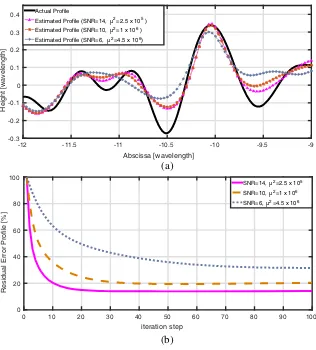
Abscissa [wavelength]
-12 -11.5 -11 -10.5 -10 -9.5 -9
Height [wavelength]
-0.3 -0.2 -0.1 0 0.1 0.2 0.3
0.4 Actual Profile
Estimated Profile (SNR=14,µ2
=2.5 x 10⁵) Estimated Profile (SNR=10,µ2=1 x 10⁶)
Estimated Profile (SNR=6, µ2=4.5 x 10⁶)
iteration step
0 10 20 30 40 50 60 70 80 90 100
Residual Error Profile [%]
0 20 40 60 80 100
SNR=14, µ2
=2.5 x 10⁵ SNR=10, µ2
=1 x 10⁶ SNR=6, µ2
=4.5 x 10⁶ (a)
(b)
Figure 5. Inversion of noisy synthetic TE-TM data from a rough profile with statistical parameters
hrms= 0.095λ, lcor= 0.3λ: (a) comparison between the actual profile and the estimated profiles, and (b) residual error profile as a function of the iteration step. Three values of the signal-to-noise ratio are studied: 14, 10 and 6.
5. CONCLUSION
An effective inversion algorithm was proposed for reconstructing a one-dimensional perfectly conducting rough surface from electromagnetic wave scattering data. Those data correspond to the interactions between the rough surface and electric dipoles in the transition zone for both fundamental polarizations. The electric dipoles also play the role of receivers. For inversion, and contrary to several other approaches, the electromagnetic interactions are modeled rigorously following the boundary integral equation method. In such a numerical simulation, tapered waves are classically used to avoid spurious edge effects. However, localized sources in the vicinity of the surface do not radiate tapered waves. In this paper, the locally perturbated plane approach [19] was implemented to curcumvent this obstacle.
Solving the inverse scattering problem consists in determining the best estimate of the actual profile from its scattered field. We implemented the Newton-Kantorovich iterative method. The calculus of the Fr´echet derivative of the scattering operator is performed at each iteration step. Then, determining a new estimation of the profile involves the resolution of a regularized local linear inverse problem.
TM data are not redudant, and should be systematically processed together to obtain the most reliable and stable solution. With the correct cost functional that mixes TE and TM data, we can show no counterexample where single-polarization inversion overperforms dual-polarization reconstruction. These results prove that the Newton-Kantorovich method can accurately inverse very rough surfaces, with correlation length much smaller than the electromagnetic wavelength. It should be pointed out that the residual error profile after one hundred iterations remains smaller than 2.5% for a profile with root mean square slope smaller than 0.45, and smaller than 10% for RMS slope smaller than 0.75.
Robustness to noise is checked and it appears that by adjusting the regularization parameter to the noise level, we can still get good quality reconstructions even at low values of the signal-to-noise ratio. For a profile with RMS slope of 0.45, the residual error profile is 2.5% on noiseless data, 14% for a signal-to-noise ratio of 14, 20% for SNR = 10 and 31% for SNR = 6.
The inversion scheme presented in this paper can directly be applied to microwave measurements on metallic surfaces with an invariance direction. The first improvement that can enhance the practicality of the algorithm is to modelize the scattering diagram of the antennas. This is particularly easy and meaningfull for the direct field between antennas. Extension to bad conductors or dielectrics, transparent or lossy, in the microwave regime is also at hand, since boundary integral equations and associated Fr´echet operators exist for such boundary condictions. Finally, our approach is not limited to two-dimensional scattering. Numerical solutions for the forward problem on two-dimensional surfaces can be coupled to the locally perturbated plane approach [19]. However, with antennas on a grid and a two-dimensional surface, the size of matrix D in the iterative process (Section 3) turns so large that specific numerical developments are to be planned.
REFERENCES
1. Ulaby, F. T., R. K. Moore, and A. K. Fung, Microwave Remote Sensing: Radar Remote Sensing and Surface Scattering and Emission Theory, Vol. II, Reading, Artech House, MA, 1982.
2. Leach, R., Optical Measurement of Surface Topography, Springer, 2011.
3. Kress, R. and T. Tran, “Inverse scattering for a locally perturbed half-plane,” Inverse Problems, Vol. 16, No. 5, 1541, 2000.
4. Tikhonov, A. and V. Arsenin, Solutions of Ill-posed Problems, Scripta Series in Mathematics, Winston, 1977.
5. Elfouhaily, T. and C. A. Gu´erin, “A critical survey of approximate scattering wave theories from random rough surfaces,” Waves in Random Media, Vol. 14, R1–R40, 2004.
6. Mendez, O., A. Roger, and D. Maystre, “Numerical solution for an inverse scattering problem of non-periodic rough surfaces,”Applied Physics B: Lasers and Optics, Vol. 32, No. 4, 199–206, 1983. 7. Wombell, R. and J. A. DeSanto, “The reconstruction of shallow rough-surface profiles from
scattered field data,”Inverse Problems, Vol. 7, No. 1, L7, 1991.
8. Afifi, S. and M. Diaf, “Scattering by random rough surfaces: Study of direct and inverse problem,”
Optics Communications, Vol. 265, No. 1, 11–17, 2006.
9. Wombell, R. and J. DeSanto, “Reconstruction of rough-surface profiles with the Kirchhoff approximation,” Journal of the Optical Society of America A, Vol. 8, No. 12, 1892–1897, 1991. 10. Sheppard, C., “Imaging of random surfaces and inverse scattering in the Kirchoff approximation,”
Waves in Random Media, Vol. 8, No. 1, 53–66, 1998.
11. Schatzberg, A. and A. J. Devaney, “Rough surface inverse scattering within the rytov approximation,” JOSA A, Vol. 10, No. 5, 942–950, 1993.
12. Cmielewski, O., H. Tortel, A. Litman, and M. Saillard, “A two-step procedure for characterizing obstacles under a rough surface from bistatic measurements,” IEEE Transactions on Geoscience and Remote Sensing, Vol. 45, No. 9, 2850–2858, 2007.
13. Ogilvy, J. A., Theory of Wave Scattering from Random Rough Surfaces, Adam Hilger, Bristol, 1991.
15. Chew, W., M. Tong, and B. Hu,Integral Equation Methods for Electromagnetic and Elastic Waves, Morgan & Claypool, 2008.
16. Arhab, S., G. Soriano, K. Belkebir, A. Sentenac, and H. Giovannini, “Full wave optical profilometry,” JOSA A, Vol. 28, No. 4, 576–580, 2011.
17. Arhab, S., H. Giovannini, K. Belkebir, and G. Soriano, “Full polarization optical profilometry,”
JOSA A, Vol. 29, No. 8, 1508–1515, 2012.
18. El-Shenawee, M. and E. L. Miller, “Multiple-incidence and multifrequency for profile reconstruction of random rough surfaces using the 3-D electromagnetic fast multipole model,”IEEE Transactions on Geoscience and Remote Sensing, Vol. 42, No. 11, 2499–2510, 2004.
19. Spiga, P., G. Soriano, and M. Saillard, “Scattering of electromagnetic waves from rough surfaces: A boundary integral method for low-grazing angles,” IEEE Trans. Antennas Propag., Vol. 56, 2043–2050, 2008.
20. Meier, A. and S. Chandler-Wilde, “On the stability and convergence of the finite section method for integral equation formulations of rough surface scattering,” Mathematical Methods in the Applied Sciences, Vol. 24, No. 4, 209–232, 2001.
21. Kantorovich, L., “On Newton’s method for functional equations,”Dokl. Akad. Nauk SSSR, Vol. 59, 1237–1240, 1948.
22. Roger, A., “Newton-Kantorovitch algorithm applied to an electromagnetic inverse problem,”IEEE Transactions on Antennas and Propagation, Vol. 29, No. 2, 232–238, 1981.
23. Roger, A., “Reciprocity theorem applied to the computation of functional derivatives of the scattering matrix,”Electromagnetics, Vol. 2, No. 1, 69–83, 1982.
![Figure 2. The last iteration step residual error profile as a function of the profile correlation lengthlcor ∈ [0.15; 0.5] for a profile height root mean square of hrms = 0.095λ: (a) inversions of the TE dataset, of the TM data set, and of the combined TE-TM data sets, and (b) zoom on inversions of the TEdata set and of the combined TE-TM data sets.](https://thumb-us.123doks.com/thumbv2/123dok_us/1987351.1262850/6.612.151.470.328.677/iteration-residual-prole-correlation-lengthlcor-inversions-inversions-combined.webp)
![Figure 3. The last iteration step residual error profile as a function of the profile height root meansquare hrms, ∈ [0.08λ; 0.14λ] for a correlation length lcor = 0.2λ: inversions of the combined TE-TMdata sets.](https://thumb-us.123doks.com/thumbv2/123dok_us/1987351.1262850/7.612.154.470.355.499/iteration-prole-function-prole-meansquare-correlation-inversions-combined.webp)