Optimal Design of Magnetically Levitated Permanent-Magnet
Planar Motors Using THD
2DMethod
Xinhua Zhang1, *, Hao Luo1, Zebin Yang1, Xiaodong Sun1, and Jinchun Hu2
Abstract—In order to reduce the higher harmonic component of the magnetic field in magnetically levitated permanent-magnet planar motors (PMPMs), a sinusoidal index for 2-dimensional (2D) wave is proposed and verified by calculating the average total harmonic distortion (THD) of the discrete
waveform. Based on this, a novel optimal design method using THD for 2-dimensional wave (THD2D)
and fundamental amplitude is proposed for PMPMs. The finite element analysis and experimental results show that the higher harmonic component of magnetic field is reduced with average fundamental amplitude invariant, and the back-EMF is better. So the optimal design method can improve the electromagnetic performance of magnetically levitated PMPMs.
1. INTRODUCTION
With requirements of high acceleration and high precision for direct planar motions, planar motors have been paid more and more attention in the academic and engineering field [1–3]. Planar motors can be classified into three categories, i.e., induction planar motors, sawyer motors and permanent-magnet synchronous planar motors [4]. Induction planar motors are made in laboratory level. Sawyer motors have some disadvantages such as heating problem and requirement of precisely manufactured teeth [5]. With the development of rare-earth permanent-magnet material, permanent-magnet synchronous planar motors attract widespread attention. Permanent-magnet synchronous planar motors can realize large-range planar motion with high speed and high precision. Usually permanent-magnet synchronous planar motors have either moving magnets and stationary coils, or moving coils and stationary magnets. The mover of planar motor is controlled in six degrees of freedom and magnetically levitated by the Lorentz force generated between the mover and stator [6].
In order to improve the dynamic performance of permanent-magnet motors, many analysis and optimization methods have been proposed. In [7, 8], the analytical expression of the magnetic field created by a radially magnetized tile permanent magnet was proposed. In [9], on the basis of magnetic vector potential, the analytical solutions for magnetic field were derived. In [10], a new technique using the hybridization of finite element analysis and permeance network method was proposed, and then a multi-objective optimization method was performed to reduce cogging torque and increase torque capability. When the acceleration for magnet array was chosen as objective, an optimization method
for the sizes of the N-S array and Halbach array under different topologies and load conditions was
proposed in [11]. In order to obtain a sinusoidal distribution of air gap magnetic field, an extra 2D analytical method was proposed in [12]. In [13], a new 2D magnet array for planar motors was proposed, and the harmonic model was developed to predict the flux density of this array. In [14], to minimize the resistive loss, geometrical optimization and parametric search were performed. In addition, many important issues, such as thrust and real-time control, were also concerned [15–18]. However, there is not much research on the optimization of Halbach magnetic field in PMPMs.
Received 3 February 2015, Accepted 30 March 2015, Scheduled 6 April 2015
* Corresponding author: Xinhua Zhang ([email protected]).
1 School of Electrical and Information Engineering, Jiangsu University, 301 Xuefu Road, Zhenjiang 212013, China.2 Department of
The stator of magnetically levitated PMPMs with moving coils adopts Halbach array [19], which can increase the amplitude but decrease the distortion of the magnetic flux density. In order to increase the thrust density and decrease the difficulty of control, the air gap flux density must be as large as possible while making the magnetic distribution close to a sinusoidal wave. The magnetic surface charge model and harmonic model have been proposed in literatures. The magnetic surface charge model can predict magnetic field accurately, but the calculation is very complicated and the simulation is time-consuming [20]. However, the harmonic model is based on the Fourier transform, and it can evaluate the magnetic field in a short time. A 3-dimensional (3D) harmonic model of the mover in magnetically levitated PMPMs with moving magnets was proposed in [21, 22], and it presented a scheme that the width of slave magnets is half of the master magnets. As a result, the magnetic flux distribution does not contain a third harmonic component. If the PMPM is driven by a balanced three-phase sine-wave current, the third harmonic component will not work, and the higher harmonic component is still high. Therefore, it is necessary to give a new optimization scheme to reduce the harmonic component.
This paper proposes a novel optimization scheme that utilizes THD2D and fundamental amplitude
to optimize the magnetic field in magnetically levitated PMPMs. Because the calculation is simple, the optimization scheme can give a better result and reflect the performance of the magnetic field in a short time. According to the result of the optimization scheme, the research prototype and simulation model confirm that the magnetic field and back-EMF are better than before.
This paper is organized as follows. The basic operation principle of magnetically levitated PMPMs is introduced in Section 2. The harmonic model of magnetic flux density is briefly described in Section 3. In Section 4, the 3D map of the magnetic field is exhibited. The sinusoidal index for 2D wave and its verification is proposed in Section 5, and the quality indicator, utilizing sinusoidal index, is also proposed. Then in Section 6, the finite element and experimental results are used to verify the proposed optimization scheme. Finally, a conclusion is drawn in Section 7.
2. OPERATION PRINCIPLE OF THE PLANAR MOTOR
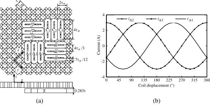
The magnetically levitated PMPM with moving coils consisting of mover and stator is shown in Figure 1(a). The stationary magnets glued to an aluminum plate adopt Halbach permanent-magnet
array. The cube magnets magnetized in thez-direction are master magnets, and meanwhile the rectangle
magnets magnetized in the x- or y-direction are slave magnets. For the existence of Halbach array, the magnetic flux density on one side of the magnet array is enhanced. The coils are placed at an angle of
45◦ with respect to the magnets and divided into 4 sets of three-phase coil (A, B, C and D), and they
are a team. The size of the coil is shown in Figure 1(a). The coils can be controlled with six degrees of freedom when they are magnetically levitated upon the permanent-magnet array. Figure 1(b) shows the current in set-A when it is working. The current in each coil is dependent on the position of the
+ + + + + + + + + + + + + + + + + + + + + + + +
+ + + + + +
+ + + +
+
n 2τ
m
z
+ + + + +
+ + +
+ + +
+ +
+ + + +
+ + +
x
y
x
n 4τ
1
D
2
D
3
D
1C2C3
C
1
B2 B3
B
1A2A3
A
n 7τ /12
n 4τ /3
0.283τ
0 45 90 135 180 225 270 315 360 Coil displacement (°)
iA2 iA3 iA1
(a) (b)
τ τ
-4 -2 0 2 4
Current (A)
air Region 3
air
permanent magnet b
Region 2
Region 1
coil
y
z x
z= -∞
z=-m
z=+∞
z=0
Figure 2. Three regions of model.
mover with respect to the stator and each coil must be energized individually. The control scheme is very difficult because all six degrees of freedom must be controlled and coupling exists between them. When coils are energized, the electromagnetic force and torque, which drive the mover in any direction, can be calculated by Lorentz law.
3. HARMONIC MODEL
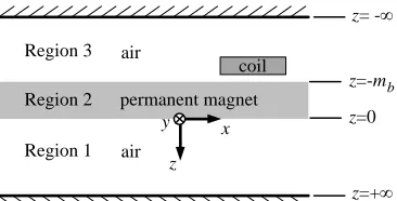
To get the expression of magnetic flux density around magnet array, the analytical model of the stator, as shown in Figure 2, is developed. Magnetic field in region 3 is enhanced. According to [21], and set
α=πx/τ and β =πy/τ, the magnetic flux density distributes in region 3 is
B3 =
⎡ ⎣BB33xy
B3z
⎤ ⎦=−μ0
∞
p=1
∞
q=1
K3(p, q)ezλ(p,q)
⎡ ⎢ ⎢ ⎣
pπ
τ cos (pα) sin (qβ) qπ
τ sin (pα) cos (qβ) λ(p, q) sin (pα) sin (qβ)
⎤ ⎥ ⎥
⎦ (1)
wherepand q are the harmonic numbers forx-,y- andz-direction. Br is the remanence of
permanent-magnet, μ0 the permeability of vacuum,mb the thickness of permanent-magnets,τ the pole pitch, τm
the length of master magnets, and
K3(p, q) =Br 1−embλ(p,q)
bpbqπp2+q2+apbqp τ λ(p, q) +aqbpqτ λ(p, q) 2 (p2+q2)πμ
0λ(p, q)
ap=pπ4 cos pτ2mτπ
sin pπ
2
, aq= qπ4 cos qτ2mτπ
sin qπ
2
bp= 4
pπsin
pτmπ
2τ
sin pπ
2
, bq = 4
qπsin
qτmπ
2τ
sin qπ
2
λ(p, q) = pπ τ
2
+ qπ
τ
2
, τn= √τ
2
It can be seen from (1) that B3 is a function of x,y and z. The harmonic numbers forx-,y- and z-directions change from 1 to ∞. The amplitude of B3 exponentially decreases in the z-direction and
trigonometrically changes in the x- and y-directions.
4. MAGNETIC FIELD DISTRIBUTION
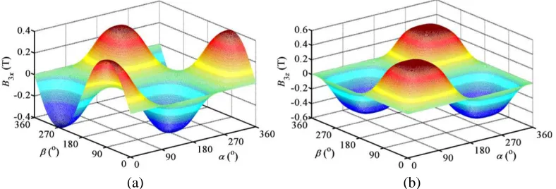
The 3D map of magnetic flux density is obtained when τ = 24 mm, τm = 16 mm and mb = 10 mm.
(a) (b)
Figure 3. The 3D map of magnetic flux density when z =−10 mm. (a) In x- (y-) direction. (b) In z-direction.
(a) (b)
Figure 4. The 3D map of magnetic flux density when z =−14 mm. (a) In x- (y-) direction. (b) In z-direction.
5. OPTIMIZATION SCHEME 5.1. Sinusoidal Index
Since the magnetic field has a significant impact on the electromagnetic force and torque, and the harmonic distortion of the magnetic field near the permanent-magnet is serious, it is important to optimize the size of permanent-magnet to enhance the magnetic field.
Traditionally, the THD for 1-dimensional periodic wave Gis THD1D(G), and it can be described
as
THD1D(G) =
∞
h=2 G2(h)
G(1) (2)
wherehis the harmonic number,G(h) the amplitude of each harmonic, andG(1) fundamental amplitude of waveform.
Since 2D waveform trigonometrically changes in the x- and y-directions, the THD in (2) is not
suitable for this case. In order to resolve this problem, a sinusoidal index for 2D wave as Equation (1) is given as
THD2D=
∞
q=2
F2(1, q) + ∞
p=2
F2(p,1) + ∞
p=2
∞
q=2
F2(p, q)
where F(1, q), F(p,1) and F(p, q) are the amplitudes of each harmonic, and F(1,1) is fundamental amplitude of the 2D waveform.
5.2. Sinusoidal Index Verification
In order to verify the correctness of the sinusoidal index, the waveform is analyzed by using fast Fourier transform. THDav is defined as the average of the THD1D in [0, π],
THDav=
⎡
⎣THDTHDavavxy
THDavz
⎤ ⎦= ⎡ ⎢ ⎢ ⎢ ⎢ ⎢ ⎢ ⎣ 1 π π 0
THD1D(B3x(β)) dβ
1 π
π
0
THD1D(B3y(α)) dα
1 π
π
0
THD1D(B3z(β)) dβ
⎤ ⎥ ⎥ ⎥ ⎥ ⎥ ⎥ ⎦ (4)
where THDavx, THDavyand THDavzare the values of THDavin thex-,y- andz-directions, respectively.
THD1D(B3x(β)), THD1D(B3y(α)) and THD1D(B3z(β)) are the THD1D(G) of different waves withαorβ
different andzconstant in thex-,y- and z-directions, respectively. SinceB3x,B3y andB3z periodically
change as shown in Figures 3 and 4, α and β are required only between 0 andπ.
To simplify the calculation, discretization will be applied to THDav. Meanwhile, [0, π] is divided
intoM subintervals averagely, where M is an integer. In this case, (4) is expressed as
THDav=
⎡
⎣THDTHDavavxy
THDavz
⎤ ⎦= 1
M ⎡ ⎢ ⎢ ⎢ ⎢ ⎢ ⎢ ⎢ ⎢ ⎢ ⎣ M m=0
THD1D B3x m
Mπ
M
m=0
THD1D B3y m
Mπ
M
m=0
THD1D B3z m
Mπ ⎤ ⎥ ⎥ ⎥ ⎥ ⎥ ⎥ ⎥ ⎥ ⎥ ⎦ (5)
According to (1) and (3), THD2D can be described as
THD2D=
THD
2Dx
THD2Dy
THD2Dz
= ⎡ ⎢ ⎢ ⎢ ⎢ ⎢ ⎢ ⎢ ⎢ ⎢ ⎢ ⎢ ⎣ ∞
p=2(−μ0K3(p,1)e
zλ(p,1)pπ τ )
2
+∞
q=2(−μ0K3(1,q)e zλ(1,q)π
τ) 2 +∞ p=2 ∞
q=2(−μ0K3(p,q)e zλ(p,q)pπ
τ ) 2
−μ0K3(1,1)ezλ(1,1)πτ
∞
p=2(−μ0K3(p,1)e zλ(p,1)π
τ)2+
∞
q=2(−μ0K3(1,q)e zλ(1,q)qπ
τ )2+
∞
p=2
∞
q=2(−μ0K3(p,q)e zλ(p,q)qπ
τ )2 −μ0K3(1,1)ezλ(1,1)πτ
∞
p=2(−μ0K3(p,1)e
zλ(p,1)λ(p,1))2+∞
q=2(−μ0K3(1,q)e
zλ(1,q)λ(1,q))2+∞
p=2
∞
q=2(−μ0K3(p,q)e
zλ(p,q)λ(p,q))2
−μ0K3(1,1)ezλ(1,1)λ(1,1)
⎤ ⎥ ⎥ ⎥ ⎥ ⎥ ⎥ ⎥ ⎥ ⎥ ⎥ ⎥ ⎦ (6)
where THD2Dx, THD2Dyand THD2Dzare the value ofTHD2Din thex-,y- andz-direction, respectively.
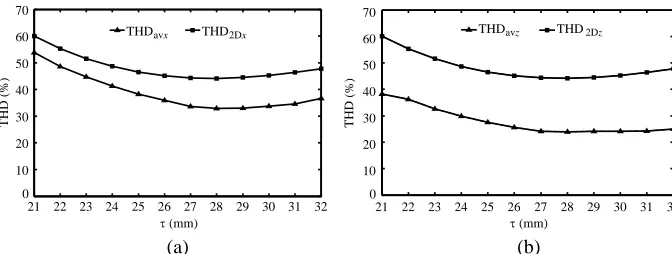
The relationships between THD and τ can be calculated by (5) and (6). Figure 5 shows their
relationships in x- (y-) direction and in z-direction. It can be seen from Figure 5 that THD2D and
THDav have the same trend in the x- (y-) and z-directions, and get the minimum when τ = 28 mm.
Therefore, the quality of a waveform can be evaluated by THD2D.
5.3. Quality Indicator
The amplitude of a waveform should be as large as possible, and its THD2Dshould be as small as possible.
21 22 23 24 25 26 27 28 29 30 31 32
THDavx THD2Dx
21 22 23 24 25 26 27 28 29 30 31 32
THDavz THD2Dz
0 10 20 30 40 50 60 70 THD (%) 0 10 20 30 40 50 60 70 THD (%) (a) (b)
τ (mm) τ (mm)
Figure 5. Relationships on THD−τ. (a) In x- (y-) direction. (b) In z-direction.
amplitude and sinusoidal index. It can be described as
Kwqi =
⎡ ⎣KKwqiwqixy
Kwqiz
⎤ ⎦= 1
hz ⎡ ⎢ ⎢ ⎢ ⎢ ⎢ ⎢ ⎢ ⎢ ⎣
−mb−hz
−mb
F Ax(z)
THD2Dx(z)dz
−mb−hz
−mb
F Ay(z)
THD2Dy(z)dz
−mb−hz
−mb
F Az(z)
THD2Dz(z)dz
⎤ ⎥ ⎥ ⎥ ⎥ ⎥ ⎥ ⎥ ⎥ ⎦ (7)
whereKwqix,Kwqiy andKwqizare quality indicators in thex-,y- andz-directions, respectively. F Ax(z), F Ay(z) and F Az(z) are the different fundamental amplitudes with z different in the x-, y- and z -directions, respectively, and their value is corresponding to F(1,1). THD2Dx(z), THD2Dy(z) and
THD2Dz(z) are different values of THD2D with z different in the x-, y- andz-directions, respectively.
hz is the distance between the top of the measurement domain and the top of the magnets. According
to the requirement of the waveform optimization, the greater the value ofKwqi is, the better the wave
is.
The domain [−mb, −mb−hz] is divided into N subintervals averagely, where N is an integer.
(7) can be expressed as
Kwqi =
⎡ ⎣KKwqiwqixy
Kwqiz
⎤ ⎦= 1
N ⎡ ⎢ ⎢ ⎢ ⎢ ⎢ ⎢ ⎢ ⎢ ⎢ ⎢ ⎢ ⎢ ⎢ ⎢ ⎢ ⎢ ⎢ ⎢ ⎢ ⎢ ⎣ N n=0 F Ax
−nhz
N −mb
THD2Dx
−nhz
N −mb
N
n=0 F Ay
−nhz
N −mb
THD2Dy
−nhz
N −mb
N
n=0 F Az
−nhz
N −mb
THD2Dz
−nhz
N −mb
⎤ ⎥ ⎥ ⎥ ⎥ ⎥ ⎥ ⎥ ⎥ ⎥ ⎥ ⎥ ⎥ ⎥ ⎥ ⎥ ⎥ ⎥ ⎥ ⎥ ⎥ ⎦ (8)
The relationships between wave quality indicator andτ in x- (y-) direction and z-directions when
τm = 16 mm, mb = 10 mm and hz = 8 mm are shown in Figure 6. It can be seen thatKwqi takes the
maximum value whenτ = 26 mm.
6. VERIFICATION
determined by the proposed quality indicator. Considering the amplitude of the magnetic field, the pole
pitch of prototype 2 is 26 mm instead of 28 mm even though the THD2D is minimum whenτ = 28 mm,
which can be seen from Figure 5. The number of turns is 175. The material of permanent magnet is NdFe30, and the simulation model is developed by finite element method. Prototype 2 is manufactured for the verification of optimization scheme. Figure 7 shows a photo of prototype 2.
6.1. Magnetic Field
Figures 8 and 9 show the waveform and harmonic analysis results of B3x and B3z, which are
1-dimensional periodic waves when z =−12 mm andβ = 30◦. It can be seen that the THD1D(B3x(β))
of prototype 1 is 18.88%, and the fundamental amplitude is 0.32 T. Meanwhile, the THD1D(B3x(β)) of
prototype 2 is 13.75%, and the fundamental amplitude is 0.30 T. In thez-direction, the THD1D(B3z(β))
of prototype 1 is 12.25%, and the fundamental amplitude is 0.52 T, while the THD1D(B3z(β)) of
prototype 2 is 8.08%, and the fundamental amplitude is 0.49 T. It is obvious that the fundamental amplitude of prototype 1 is slightly larger than that of prototype 2, but the inhibitory effect on higher
21 22 23 24 25 26 27 28 29 30 31 32 21 22 23 24 25 26 27 28 29 30 31 32
Kwqi
z
Kwq
ix
(a) (b)
τ (mm) τ (mm) 1
1.4 1.8 2.2 2.6 3
0 0.4 0.8 1.2 1.6 2
Figure 6. Relationships on wave quality indicator andτ. (a) In x- (y-) direction. (b) In z-direction.
Prototype 1 Prototype 2
τ (mm) 24 26
τm (mm) 16 16
mb (mm) 10 10
Table 1. Magnet parameters.
(a) (b)
Figure 7. Photo of prototype 2. (a) Permanent-magnet array. (b) Coils.
0 45 90 135 180 225 270 315 360
α (°)
Prototype 1 Prototype 2
(a) (b)
-0.4 -0.3 -0.2 -0.1 0.1 0.2 0.3 0.4
B
(T)
3
x 0
0 45 90 135 180 225 270 315 360
Prototype 1 Prototype 2
(a) (b)
-0.6 -0.4 -0.2 0 0.2 0.4 0.6
B
(T)
3
z
α (°)
Figure 9. Comparison ofB3z whenz=−12 mm and β= 30◦. (a) Waveform. (b) Harmonic analysis.
(a) (b)
Figure 10. Comparison inx- (y-) direction. (a) THD1D(B3x(β)). (b) Fundamental amplitude.
(a) (b)
Figure 11. Comparison inz-direction. (a) THD1D(B3z(β)). (b) Fundamental amplitude.
harmonics of prototype 2 is better than that of prototype 1.
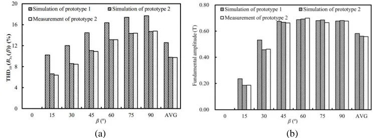
To further investigate their magnetic field distribution, the considered domain is divided into finite subintervals, such as 0◦, 15◦, 30◦, 45◦, 60◦, 75◦ and 90◦. When z = −12 mm, prototypes 1 and 2 are both 1-dimensional periodic waves. The predicted and measured results for prototypes 1 and 2 are given in Figures 10 and 11. The THD1D(B3x(β)) and fundamental amplitude in x- (y-) direction are shown
in Figure 10. It can be seen that prototype 1 has a higher average THD1D(B3x(β)) than prototype 2.
In addition, they have almost the same average fundamental amplitude. The measurement result of prototype 2 agrees with its predicted one if the error of measurement is ignored. The THD1D(B3z(β))
and fundamental amplitude in z-direction are shown in Figure 11, and the situation is the same as
x-direction.
0 45 90 135 180 225 270 315 360
Coil displacement (°)
Simulation of prototype 1 Simulation of prototype 2 Measurement of prototype 2
(a) (b)
-2 -1.5 -1 -0.5 0 0.5 1 1.5 2
Ba
c
k
-E
M
F
(V
)
Figure 12. Back-EMF of one coil and its harmonic analysis. (a) The back-EMF. (b) Harmonic analysis.
6.2. Back-EMF
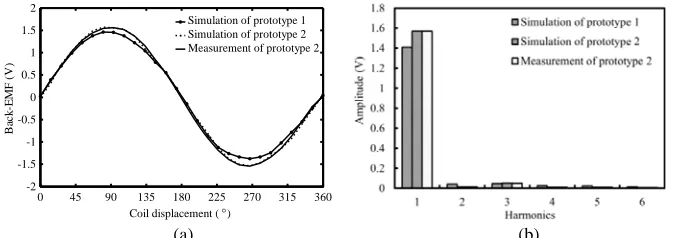
Figure 12 shows the back-EMF of one coil when the coil moves along a direction perpendicular to the coil. The speed is 300 mm/s, and the length of air-gap is 1 mm. The back-EMF of one coil is measured by an oscilloscope. It can be seen that the simulated and measured values of prototype 2 match each other well. The peak simulation value of prototype 1 is 1.41 V, and that of prototype 2 is 1.57 V. It should be noted that the coils become longer after optimization. To further investigate the difference between the two prototypes, the simulation results are analyzed using Fourier transform. The results show that the
THD1D of prototype 1 is 5.61%, and that of prototype 2 is 3.42%, it is means that the performance of
prototype 2 is slightly better than prototype 1. It should be noted that since the distortion of magnetic
field decreases with the increase of the distance from magnet surface, the difference between the THD1D
of back-EMF generated by the coils of two prototypes is smaller than that in the magnetic field of the two prototypes.
7. CONCLUSION
According to the harmonic model of the magnet array in the magnetically levitated PMPMs, the magnetic field distribution has been analyzed, and a sinusoidal index for 2D wave has been proposed and verified. By utilizing the sinusoidal index and fundamental amplitude, a wave quality indicator which can easily describe the performance of the waveform has also been proposed. Compared with the existing optimization method, the proposed scheme has a lower THD and keeps the average fundamental amplitude invariant, and the back-EMF is better. It means that this method can improve the electromagnetic performance of PMPMs. Finally, the effectiveness of the proposed optimal design method has been verified by the finite element analysis and experimental results.
ACKNOWLEDGMENT
This work was supported by the National Natural Science Foundation of China (Projects 51475214, 51305170 and 51175296), by the 2011 Jiangsu Regular High School Postgraduate Students’ Scientific Research Innovation Program (Project CXLX11 0585) and by the Priority Academic Program Development of Jiangsu Higher Education Institutions.
REFERENCES
1. Compter, I. J., “Electro-dynamic planar motor,” Precision Engineering, Vol. 28, No. 2, 171–180,
2004.
2. Min, W., M. Zhang, Y. Zhu, F. Liu, G. Duan, J. Hu, and W. Yin, “Analysis and design of novel overlapping ironless windings for planar motors,”IEEE Transactions on Magnetics, Vol. 47, No. 11, 4635–4642, 2011.
3. Rovers, J. M. M., J. W. Jansen, J. C. Compter, and E. A. Lomonova, “Analysis method of the dynamic force and torque distribution in the magnet array of a commutated magnetically levitated
4. Cho, H.-S. and H.-K. Jung, “Analysis and design of synchronous permanent-magnet planar motors,” IEEE Transactions on Energy Conversion, Vol. 17, No. 4, 492–499, 2002.
5. Cho, H.-S., C.-H. Im, and H.-K. Jung, “Magnetic field analysis of 2-D permanent magnet array for
planar motor,” IEEE Transactions on Magnetics, Vol. 37, No. 5, 3762–3766, 2001.
6. Choi, J. H., J. H. Park, and Y. S. Baek, “Design and experimental validation of performance for
a Maglev moving-magnet-type synchronous PM planar motor,”IEEE Transactions on Magnetics,
Vol. 42, No. 10, 3419–3421, 2006.
7. Ravaud, R. and G. Lemarquand, “Comparison of the coulombian and amperian current models for calculating the magnetic field produced by radially magnetized arc-shaped permanent magnets,” Progress In Electromagnetics Research, Vol. 95, 309–327, 2009.
8. Ravaud, R., G. Lemarquand, V. Lemarquand, and C. Depollier, “The three exact components
of the magnetic field created by a radially magnetized tile permanent magnet,” Progress In
Electromagnetics Research, Vol. 88, 307–319, 2008.
9. Kang, H. B., J. Y. Choi, H. W. Cho, and J. H. Kim, “Comparative study of torque analysis for synchronous permanent magnet coupling with parallel and halbach magnetized magnets based on analytical field calculations,” IEEE Transactions on Magnetics, Vol. 50, No. 11, 8600604, 2014. 10. Touati, S., R. Ibtiouen, O. Touhami, and A. Djerdir, “Experimental investigation and optimization
of permanent magnet motor based on coupling boundary element method with permeances
network,” Progress In Electromagnetics Research, Vol. 111, 71–90, 2011.
11. Boeij, J., E. Lomonova, and A. Vandenput, “Modeling ironless permanent-magnet planar actuator
structures,”IEEE Transactions on Magnetics, Vol. 42, No. 8, 2009–2016, 2006.
12. Jing, L., L. Liu, M. Xiong, and D. Feng, “Parameters analysis and optimization design for a
concentric magnetic gear based on sinusoidal magnetizations,” IEEE Transactions on Applied
Superconductivity, Vol. 24, No. 5, 0600905, 2006.
13. Min, W., M. Zhang, Y. Zhu, B. Chen, G. Duan, J. Hu, and W. Yin, “Analysis and optimization
of a new 2-D magnet array for planar motor,” IEEE Transactions on Magnetics, Vol. 46, No. 5,
1167–1171, 2010.
14. Boeij, J., E. A. Lomonova, and A. J. Vandenput, “Optimization of contactless planar actuator with
manipulator,”IEEE Transactions on Magnetics, Vol. 44, No. 6, 1118–1121, 2008.
15. Cao, J., S. Wang, Y. Zhu, and W. Yin, “Modeling the static vertical force of the core-type
permanent-magnet planar motor,” IEEE Transactions on Magnetics, Vol. 44, No. 12, 4653–4658,
2008.
16. Cao, J., Y. Zhu, J. Wang, W. Yin, and G. Duan, “A novel synchronous permanent magnet planar
motor and its model for control applications,” IEEE Transactions on Magnetics, Vol. 41, No. 6,
2156–2163, 2005.
17. Peng, J., Y. Zhou, and G. Liu, “Calculation of a new real-time control model for the magnetically levitated ironless planar motor,”IEEE Transactions on Magnetics, Vol. 49, No. 4, 1416–1422, 2013. 18. Rovers, H., J. W. Jansen, and E. A. Lomonova, “Multiphysical analysis of moving-magnet planar
motor topologies,” IEEE Transactions on Magnetics, Vol. 49, No. 12, 5730–5741, 2013.
19. Yan, L., L. Zhang, T. Wang, Z. Jiao, C.-Y. Chen, and I.-M. Chen, “Magnetic field of tubular linear machines with dual halbach array,”Progress In Electromagnetics Research, Vol. 136, 283–299, 2013. 20. Jansen, J. W., J. P. C. Smeets, T. T. Overboom, J. M. M. Rovers, and E. A. Lomonova, “Overview
of analytical models for the design of linear and planar motors,”IEEE Transactions on Magnetics,
Vol. 50, No. 11, 8206207, 2014.
21. Jansen, J. W., C. M. M. Van Lierop, E. A. Lomonova, and A. J. A. Vandenput, “Modeling of
magnetically levitated planar actuator with moving magnets,” IEEE Transactions on Magnetics,
Vol. 43, No. 1, 15–25, 2007.
22. Jansen, J. W., C. M. M. Van Lierop, E. A. Lomonova, and A. J. A. Vandenput, “Magnetically
levitated planar actuator with moving magnets,” IEEE Transactions on Industry Applications,