Geological Object Recognition in Extraterrestrial Environments

(1)

Western University Western University

Scholarship@Western

Electronic Thesis and Dissertation Repository

4-16-2015 12:00 AM

Geological Object Recognition in Extraterrestrial Environments

Gregory M. Elfers

The University of Western Ontario Supervisor

Dr. Olga Veksler

The University of Western Ontario Graduate Program in Computer Science

A thesis submitted in partial fulfillment of the requirements for the degree in Master of Science © Gregory M. Elfers 2015

Follow this and additional works at: https://ir.lib.uwo.ca/etd

Part of the Artificial Intelligence and Robotics Commons, Geology Commons, and the Other Computer Sciences Commons

Recommended Citation Recommended Citation

Elfers, Gregory M., "Geological Object Recognition in Extraterrestrial Environments" (2015). Electronic Thesis and Dissertation Repository. 2822.

https://ir.lib.uwo.ca/etd/2822

This Dissertation/Thesis is brought to you for free and open access by Scholarship@Western. It has been accepted for inclusion in Electronic Thesis and Dissertation Repository by an authorized administrator of

(2)

GEOLOGICAL OBJECT RECOGNITION IN EXTRATERRESTRIAL

ENVIRONMENTS

(Thesis format: Monograph)

by

Greg Elfers

Graduate Program in Computer Science

A thesis submitted in partial fulfillment

of the requirements for the degree of

Masters of Science

The School of Graduate and Postdoctoral Studies

The University of Western Ontario

London, Ontario, Canada

c

(3)

Acknowlegements

I would like to acknowledge Melissa Elfers, my wife, who graciously shares me with my computer, but still loves me more than my computer ever has. Dr. Olga Veksler who probably didn’t realize what she was getting into when she agreed to supervise me. My sister Cynthia, whose patience with me in this life has gone far beyond what siblings should have to endure and Stacy “Spacey” Orsat, who helped me start down the road to university. Owen McCarthy, who spent many hours beside me in undergrad, listening to me swear at code, he protected my sanity and challenged me academically even if he was never able to get that last mark. Tom Cunningham whose example showed me that any problem could be solved with patience and determination. Dr. Steven Beauchemin who gave me an opportunity to be excited about Mathematics. Dr. Taha Kawasari who was always ready to answer a question about that math, despite being eyeball deep in his own thesis. And a special thanks to Bernard Sandler who pointed me in the direction of the end even if I’m not that good with following directions.

This thesis is also dedicated to the fond memory of:

Barbara and Manfred Elfers, The height of a building, depends on the strength of its foundation. Jane Bashara, whose encouraging light was dimmed before its time,

Dr. Sheng Yu, who showed me the beauty of computing,

Greg Mate, whose optimism during his fight against cancer put the battles I face in perspective.

(4)

Abstract

On July 4 1997, the landing of NASA’s Pathnder probe and its rover Sojourner marked the beginning of a new era in space exploration; robots with the ability to move have made up the vanguard of human extraterrestrial exploration ever since. With Sojourners landing, for the rst time, a ground traversing robot was at a distance too far from earth to make direct human control practical. This has given rise to the development of autonomous systems to improve the e?ciency of these robots,in both their ability to move,and their ability to make decisions regarding their environment. Computer Vision comprises a large part of these autonomous systems, and in the course of performing these tasks a large number of images are taken for the purpose of navigation. The limited nature of the current Deep Space Network means that a majority of these images are never seen by human eyes. This work explores the possibility of using these images to target certain features by using a combination of three AdaBoost algorithms and established image feature approaches to help prioritize interesting subjects from an ever growing data set of imaging data.

Keywords:Computer Vision, Shatter Cones, Autonomous Robotics, Machine Learning

(5)

List of Figures

1.1 Hematite spherules . . . 4

3.1 Variation in outcrop appearance . . . 10

(a) An example of a visually simple outcrop . . . 10

(b) An example of a visually complex outcrop . . . 10

3.2 Examples of shatter-cone completeness . . . 11

(a) An example of a nested shatter-cone. . . 11

(b) An example of a partially developed shatter-cone . . . 11

3.3 Shatter Cones can range in size from millimetres to meters and come in a vari-ety of orientations. . . 12

(a) A 30m Shatter-Cone from the Sudbury impact site . . . 12

(b) Hand Sized Inverted Shatter Cone from the Steinheim impact structure. . 12

3.4 Pressure-temperature Plot of Metamorphic Processes . . . 13

4.1 Various views of pens . . . 15

(a) A Bic Pen . . . 15

(b) ...With Occlusions . . . 15

(c) ...Inversely Occluded . . . 15

(d) ...Colour Inverted . . . 15

(e) ...Differently Orientated . . . 15

(f) Lollipop Pens . . . 15

4.2 A representation of a standard scale space where each dot represents an interval imagevos Whereo is the image’s octave and sis the interval. The dots in red represent the images covering the whole octave while the dots in grey are used in extrema detection. . . 17

4.3 A representation of the Difference of Gaussian(DoG) scale space where each dot represents an interval image,wo sWhere,ois the image’s octave andsis the interval. The dots in red represent the images covering the whole octave while the dots in grey supplementary images used for the extraction of candidate key points. . . 18

4.4 Extracting candidate keypoints by finding 3D Extrema. . . 18

4.5 Viola and Jones’integral imagemethod for calculating the intensity of a region using only the corner points . . . 19

4.6 Examples of Haar like features . . . 20

(a) An example of features used by Viola and Jones for face detection . . . . 20

(b) An extended feature set . . . 20

4.7 Sobel Operators . . . 21

(9)

(a) Horizontal . . . 21

(b) Vertical . . . 21

(c) NW-SE Diagonal . . . 21

(d) NE-SW Diagonal . . . 21

(e) Non-Directional . . . 21

4.8 A modern Edge Orientation Gradient . . . 21

4.9 A visual representation of the HOG feature . . . 22

(a) An image of a sports player . . . 22

(b) Visualization of HOG features . . . 22

(c) HOG Features on image . . . 22

4.10 Dalal,Triggs Process for image identification using HOG . . . 23

4.11 A visual representation of a line in Rho Theta space . . . 24

(a) Rho Theta Notation . . . 24

(b) A Point described in Polar Space . . . 24

(c) Points on a line . . . 24

4.12 Weaknesses of Intensity Histograms . . . 26

(a) Identical Intensity Histograms for dissimilar images . . . 26

(b) Susceptibility of Intensity Histograms to Lighting Changes . . . 26

(c) Rock VS. Regolith . . . 26

5.1 A visual representation of the AdaBoost algorithm . . . 31

(a) initial distributionD1 . . . 31

(b) initial hypothesish1(n) . . . 31

(c) distributionD2 . . . 31

(d) second hypothesish2(n) . . . 31

(e) distributionD3 . . . 31

(f) third hypothesish3(n) . . . 31

(g) Final HypothesisHfinal . . . 31

5.2 Underfitting vs. Overfitting . . . 32

(a) Overfitting . . . 32

(b) Underfitting . . . 32

5.3 A Simple Classification Tree example . . . 33

5.4 CART and Recursive Partitioning . . . 34

5.5 CART Model Fitting . . . 35

(a) Example DataSpace . . . 35

(b) CART Overfitting . . . 35

(c) CART Proper fit . . . 35

6.1 Field Equipment . . . 36

(a) ROC6 Rover . . . 36

(b) GigaPan Camera Mount . . . 36

6.2 Examples of the Outcrop Data Set . . . 37

(a) . . . 37

(b) . . . 37

(c) . . . 37

(10)

(d) . . . 37

(e) . . . 37

(f) . . . 37

(g) . . . 37

(h) . . . 37

6.3 Examples of the Shatter Cone Data Set . . . 39

(a) . . . 39

(b) . . . 39

(c) . . . 39

(d) . . . 39

(e) . . . 39

(f) . . . 39

(g) . . . 39

(h) . . . 39

7.1 The six Haar-like features. . . 41

7.2 The results of CART node size . . . 44

(a) Training with a decision tree with 16 nodes . . . 44

(b) Same Features as (a) but using 4 nodes . . . 44

7.3 The results of various iterations of the same data . . . 45

(a) 8 Node Tree . . . 45

(b) also an 8 node tree with the same features as (c) . . . 45

7.4 Amplitude distribution of detection window values . . . 46

(a) Gentle AdaBoost Distribution . . . 46

(b) Modest AdaBoost Distribution . . . 46

(c) Real AdaBoost Distribution . . . 46

7.5 Standard Score of the confidence distributions . . . 46

(a) Gentle Standard Score . . . 46

(b) Modest Standard Score . . . 46

(c) Real Standard Score . . . 46

7.6 Weakly and Strongly Differentiated Feature Distribution . . . 47

(a) Weakly differentiated features in an image . . . 47

(b) Strongly differentiated features in an image . . . 47

7.7 Comparison of Test Error using different subsets of features . . . 48

(a) Training with all features . . . 48

(b) Training with only Hough Transform Haar and RGB histograms . . . 48

7.8 A selection of results in positive identification of an Outcrop . . . 49

(a) Test 1 Result . . . 49

(b) Probability map of (a) . . . 49

(c) Test 2 Result . . . 49

(d) Test 2 Result . . . 49

(e) Test 3 Success . . . 49

(f) Test 3 Result . . . 49

7.9 A utter failure in the identification of Outcrops . . . 50

(a) Test 3 Novel Image . . . 50

(11)

(b) Test 3 Result . . . 50

7.10 A comparison of our Probability Method, vs. a Committee voting method . . . 51

(a) Test 4 Using Proability . . . 51

(b) Test 4 Using Committee Values . . . 51

7.11 A comparison of offsite outcrop locations . . . 52

(a) Test 5 using a local rock structure . . . 52

(b) Test 5 using a random outcrop . . . 52

7.12 Training results using a full set of features with and without the RGB histogram 52 (a) Test Error All Features . . . 52

(b) Test Error All but RGB . . . 52

7.13 The same image run with initial training data base at different section window sizes. . . 54

(a) Confidence values using 200px windows . . . 54

(b) Confidence values using 100px windows . . . 54

7.14 Typical test image used in our second Test round . . . 55

7.15 A typical test image used in test 2 of the shatter-cone images. This image was selected for shading variations and oblique surfaces relative to the camera plane. . . 56

(a) Positively weighted windows at 100px . . . 56

(b) 100px probability map. . . 56

(c) Positively weighted windows at 200px . . . 56

(d) 200px probability map. . . 56

7.16 From Left to Right: The original image. Windows labeled by our algorithm as shatter-cones. A weighted distribution of probability that the encircled image contains a shatter-cone. . . 58

(a) Shatter-cones in Sudbury Breccia . . . 58

(b) Identification of Shatter-cones . . . 58

(c) Labeled Shatter-cones . . . 58

7.17 Shatter-cone Labelling based for various sub window sizes for the same image. The smaller size windows show better resolution in identifying small as well as large shatter-cones but comes at a cost of an exponential growth in processing times. . . 59

(a) Shatter-cone Probability at 24px . . . 59

(b) Shatter-cone Probability at 100px . . . 59

7.18 Shatter-cone Labelling based for various sub window sizes for the same image. The larger window size still detect larger scale shatter-cones, but as the window size increases smaller features are lost and error creeps into textured regions due to a loss of resolution. . . 60

(a) Shatter-cone Probability at 200px . . . 60

(b) Shatter-cone Probability at 400px . . . 60

7.19 A probability map of shatter-cones in novel landscape scale image . . . 61

(a) Vredefort Dome South Africa . . . 61

(b) Slate Islands . . . 61

(c) Prince Albert Impact Crater, Victoria Island NWT . . . 61

(12)

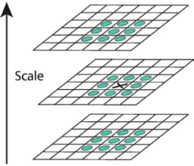
8.1 A comparison of areas of interest identified at different scales. . . 64

(a) Results at 300px . . . 64

(b) Results at 100px . . . 64

(c) Close up of positive results . . . 64

(13)

List of Tables

4.1 Sift descriptor Algorithm steps. (Adapted from Otero and Delbracio [50].) . . . 17

7.1 Overview of feature implementation . . . 41 7.2 Overview of feature effectiveness . . . 43 7.3 Shatter-cone Test Image Distribution . . . 56

(14)

Chapter 1 Introduction

1.1 Motivation

Since December 13th, 1972, when Apollo 17 Astronauts Eugene Cernan and Harrison Schmitt took their last steps on the lunar surface, the exploration of extraterrestrial environments has been the exclusive providence of robots. In recent years with the success of Pathnder/Sojourner in 1997, the Mars Exploration Rovers (MER) Spirit and Opportunity in 2003, and Mars Sci-ence Laboratory (MSL) Curiosity on August 6th 2012, the usefulness of robotic surface rovers in extraterrestrial research has been rmly established. With a number of rover missions planned for launches in the next 10 years by the space agencies of China, India, Russia, and the Eu-ropean Union, the importance of these mechanized explorers cannot be understated. Current protocols require human intervention in almost every step, but growing mission demands and improving capabilities mean that rovers are covering more distance without the assistance of humans. Pathnders rover, Sojourner, for example, traveled a total of 100 meters over the en-tirety of its 3 month mission while Opportunity has traveled over 42.23 kilometres in its 12 years on the Martian surface (slightly more than the 42.195 kilometre distance of an Olympic Marathon[40].) With the arrival of Curiosity, and an ever growing list of long duration or-biters and deep space probes, combined with the costly equipment needed for increases in the bandwidth available in the Deep Space Communication Array, autonomy for these rovers is becoming a more apparent requirement.

The rst steps of this autonomy began with the MER rovers GESTALT navigation system which helps the rover with the minutiae of driving. The next step was taken with the upload of CalTech/JPL’s AEGIS Autonomous Science software package to Opportunity in 2009. The foundation of any autonomous system rests in the ability of that system to correctly identify and di?erentiate the objects around it. The rocks on the surface of an extraterrestrial world are a rich source of information. Their location, chemical makeup, and physical structure can tell the environmental history of the body on which they sit. This is especially true in the area around craters where the violence of an impact can reveal clues otherwise hidden deep within the bedrock of a planet.

One of the largest constraints faced in the development of algorithms for this kind of work, lies in the limited computational power available to the rover. MER Opportunity has 20MHz RAD6000 Processor with 128MB of RAM and 256MB flash memory. The AEGIS system

(15)

2 Chapter1. Introduction

regularly processes 1 MB images while having access to only 4MB of RAM [27]. This means that an operation which takes mere seconds on a modern processor, will take many minutes or hours on a rover. While the MSL Curiosity rover has a processor that is an order of magnitude more powerful as the one which AEGIS runs on, it is still several orders of magnitude slower than a modern laptop. While the scope of this work will not limit itself to currently available rover processing power, it is essential that our solutions are informed by such limitations.

Despite the limitations of processing power, perhaps the most compelling argument to be made, comes from the limitations in bandwidth. At the current time any spacecraft not in earth orbit communicates with earth through NASA’s deep space communication network, which consists of three sights located 120 degrees apart on the planet, with stations in Spain, Cali-fornia, and Australia. As the capabilities of the instrumentation on each successive generation of spacecraft grows more complex, so to does the amount of data they are able to generate. Current craft such as the Lunar Reconnaissance Orbiter are expected to generate over 70 TB of data over its serviceable lifetime, Which is an order of magnitude larger than the Mars Recon-naissance Orbiter launched just a few years earlier. In order to save bandwidth current missions send low resolution image thumbnails which allows mission planners to make decisions about science targets and navigation. If mission control requires, the rover will send full resolution copies of the data on subsequent communications.

While this system works well for current missions, it means that only a small fraction of existing imagery is used. Some data, such as navigation and hazard avoidance imagery is never seen by human eyes, and of the images returned, the resolution of thumbnail data may be insufficient to capture key details contained within the rocks. Such an approach is also very slow, with the rover moving mere feet per day, transmitting imagery back to earth and then awaiting instructions on how to proceed. Ultimately it is the slow pace of this method of exploration that presents its largest drawbacks.

In its planning documents NASA has identified sample return missions as a key goal in the intermediate future. Such a mission would demand a much quicker timeline than current operating procedures allow. To maximize the effectiveness of the science on a mission of this type, a much larger area would have to be explored in greater detail more rapidly than current methods would allow. A rover with the ability to detect objects of interest in its surrounding environs would offer a great advantage in a mission such as this.

1.2 Scope of our investigation

In our investigation, we are looking at two proof of concept implementations of a method of identifying a terrain of interest, that will demonstrate the feasibility of developing generalizable feature descriptors to allow for a general image description language. Such a language would allow for a flexible method of allowing a rover to perform an unsupervised classification of specific terrain types of interest to ground based controllers. This work will incorporate a variety of image feature types despite the current limitation is extraterrestrial processing power, with the belief that such a system may be useful if the techniques investigated allow for such a system to be incorporated into the data collection methods used in the field of Terrestrial Geology.

(16)

1.3. Approach 3

special equipment or close investigation by a rover. This would allow for a program to run in conjunction with existing navigational and scientific operations, to increase the potential of scientific discovery without changing primary mission perimeters. This work will focus on two features at the scale of “Field Geophotography.” This is the scale of photos used by field geologists in their work and limit its scope to images capable of being photographed by a standard commercial point and shoot camera. For the purposes this work, this means image frames representing a distance of 20cm-100m Large landscapes will not be included except where they form the background of closer objects.

The features chosen for investigation are outcrops and shatter-cones. Outcrops were se-lected because of they represent the underlaying structure of a geological region, and may give clues as to the conditions that existed during their formation. Such structures may also be of interest in the identification of global phenomenon. And the presence of certain minerals, their deposition and erosion can give clues as to the historical conditions over a broad timescale. Such features exist with relative frequency and will almost certainly exist within the landing zone of a rover. Besides the scientific interest provided by the make up of individual examples, they are also useful as landmarks. A change in appearance of local outcrops can delineate different geological zones, or their orientation and arrangement within a landscape can suggest larger underlaying structures.

The second feature, shatter-cones, provide a unique opportunity of automated investiga-tion for a number of reasons. A shatter-cone is unique to a specific range of impact events, and present at the same time, quite unique and yet almost universal features in their appear-ance. They are indicative of a specific, set of pressures present at the time of their creation, and have been found in a variety of rock types in a number of locations on earth. As of yet these structures have not been identified on other planets, and since most imagery is returned to earth in a low resolution format that might obscure their characteristic features, they repre-sent an ideal candidate for automated detection from a rover. Shatter-cones also reprerepre-sent a tantalizing terrestrial application for locating impact craters here on earth. The Earth Impact Database maintained at the University of New Brunswick identifies only 188 confirmed impact sites, which is a fraction of the sites observed on other planets and moons.[52] The unique and macroscopic nature of this feature makes it a good candidate for identification in existing images and the mining of online photo repositories could offer clues of undiscovered impact sites.

1.3 Approach

While object detection is one of the most active fields of study in computer vision, it cannot be thought of as a routine or common place process. Very often the most successful algorithms depend on applying situational heuristic tuning or on identifying descriptors that fit well with specific features of the object being sought. An approach to face detection can be reasonably certain that the overarching design and main structural features of a human face do not vary greatly from person to person. Likewise, despite the variances in the design of cars, certain operational requirements mean that similar looking structures can be found in predictable lo-cations in an overwhelming number of the various iterations of cars.

(17)

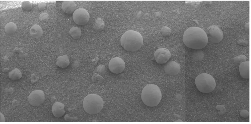
Credit:NASA

Figure 1.1: The existence of Hematite spherules found embedded in rock would illicit far less comment on earth than it did when Opportunity found these spherules at Meridiani Planum in 2004. Such structures are strong indicators of the presence of liquid water during their formation.

most of the parameters which might be used to describe an object can vary to an extraordi-nary degree. Objects with almost identical chemical makeups can vary widely in appearance. Likewise completely dissimilar objects can appear almost identical to one another on all but the microscopic level. While the morphology of a region can impose some structural simi-larities in appearance between different rock features, there are can be large variations due to the chemistry of the surrounding rocks. To complicate things further, the context of a feature within or with respect to its environment or even within the context of similar structures else-where on a planet, can change its scientific interest significantly. For example, similarities in the fossils and minerals in rocks in Africa and South America suggested that these two distant locations once touched, and an image of hematite spherules like the one in Figure 1.1 would have elicited little interest were they to have been found on Earth rather than on Mars.

In light of the complexities of this problem, and with the expectation of the availability of human expertise in the planning and execution of such missions, we have opted to develop a system in which the objects of interest are known at least to some degree,and can be pre-trained from a set of known examples. Or with the help of human expertise a training database can be constructed with a modestly sized subset of gathered examples To this end we have chosen to use the machine learning algorithm AdaBoost to train a classier from a set of feature vectors created from weak descriptors in order to create a decision making committee that is able to identify objects of interest. As we will see in our discussion in Chapter 5, a machine learning approach o?ers a number of key advantages over other methods.

(18)

1.4. Outline 5

from the same geological region but taken of different structures or from different points of view. With the shatter-cone training data we will use examples of shatter-cones from a single geographic location and attempt to apply our detection mechanisms to similar structures in widely different geological regions.

1.3.1 Program Workflow

Data Set preprocessing The process will begin by building a data set from our test images isolating just those features which are to be identified by the algorithm, a roughly equal number of negative examples from those same images will also be created. Each image in the data set will be resized to 100x100 pixels to represent different resolutions, then a histogram normal-ization algorithm is applied to the images and a greyscale version created. The appropriate image is then passed to each of the feature extractors.

Feature Extraction For the purpose of our investigations 9 different features were isolated from 7 different descriptor strategies we extracted from the image. The feature set consists of:

Scale Invariant Feature Transform(SIFT)[42] Haar like features (Haar)[63]

Histogram of Oriented Gradients(HOG)[19] Edge Orientation Gradients(EOG)[29] Hough Transforms[23]

Intensity Histograms Edge Density

Machine Learning Once the features are extracted a feature vector will be constructed and labeled as either an interesting example or an uninteresting example at which point a boosting algorithm[57] will be used to create a decision making committee to evaluate new images.

Object Identification To identify features within a novel object, a feature vector will be created from sub-windows of the image we are analyzing and a probability map of the image as a whole will be created by calculating the decision making committee’s evaluation of each sub-window.

1.4 Outline

(19)

(20)

Chapter 2 Previous Work

The use of computer vision algorithms in the field of Geology is a rapidly growing practice. Starting in the defence and space industry for use with satellite imagery, and more recently spurred on in large part by the resource extraction and processing industries who have bene-fited from technologies developed for the military’s increasing use of unmanned aerial vehicles (UAVs) automated surveying through a variety of optical and infrared techniques forms an increasingly important part of field work. Traditionally however this work has focused on ei-ther in work on large scale aerial imaging or in the realm of the microscopic for the purpose of automated mineral identification. The reasons for this can be understood in the context of the requirements of fieldwork. Terrestrial geological exploration often happens in locations where power is limited, and access is difficult. This has meant that the logistics required to insert and power a ground based system for the purpose of autonomous geology has proved more unwieldy than useful to an individual geologist in the field. In such cases where a ter-restrial location is unavailable to human exploration, the relative simplicity and reliability of teleoperation has biased remote exploration systems towards those systems. Even in Extrater-restrial environs as far away as the moon, human guided systems are much more capable than autonomous system are. It is only with the development of robotic rovers for the exploration of more distant locations such as Mars, that both the need, and operational ability have come together.

While this has been the case in the past, it is certainly not true of the future. While the rigours of space travel have demanded that computer processing power be adopted more slowly, it is now reaching a stage where reasonably complex and powerful computer systems for con-trolling autonomous identification systems are being launched. Likewise with the growth of low power processors, and the growing efficiency of power systems it is reasonable to assume that the trend will continue including the growth of more autonomous aspects of terrestrial field work. Much of the previous work focuses on one of three broad categories, landscape awareness for autonomous navigation, commonly referred to as “Simultaneous Localization and Map Building” (SLAM), rock finding algorithms for identifying protruding objects, and material identification algorithms for autonomous identification of rock composition.

(21)

8 Chapter2. PreviousWork

2.1 SLAM

SLAM techniques can be quite comprehensive in scope, but can be subdivided into three gen-eral areas, position identification, obstacle avoidance, and path finding. A lot of work has been done in this area in recent years, with the most famous terrestrial examples of such vehicles being “Stanley,” the winner of the “2005 DARPA Grand Challenge,” and Google’s “Self-driving” Car [60, 61]. Both of these vehicles make use of point clouds created by an om-nidirectional Light Detection and Ranging (LIDAR) system, and require massive amounts of computational power due to the relative speed of the vehicles. While none of the current gen-eration of rovers use LIDAR systems for navigation, the possibility is being investigated for future Rovers [2, 54]. Position identification in the context of autonomous navigation is used to locate the vehicle within its environment and to help provide more robust odometry data. Obstacle avoidance is often a realtime endeavour whose goal is to identify immediate hazards located along the direction of travel and within a relatively short range (relative to the vehicles velocity.) Pathfinding on the other hand often requires a broader, more panoramic and longer range view of the surrounding landscape and its hazards. Pathfinding can consist of both real-time and pre-plotted components choosing a prospective path between two points, and in the case of a system such as a rover, path corrections are selected as new information is provided by obstacle avoidance routines. A number of different optical techniques have been developed to this end, including land mark validation [64], Visual Odometry(VO) [44, 49], maximum likelihood matching range maps [48], and rock modelling and matching [41]. The Mars Ex-ploration Rovers (MER) Spirit and Opportunity and now The Mars Science Laboratory (MSL) Curiosity are currently using some of these techniques to help them traverse dangerous terrain. (See section 2.4.)

2.2 Rock Detection

Rock detection is an important part of operational and scientific awareness at a given loca-tion. Depending on the required definition of what constitutes an interesting rock, or even what constitutes a rock at all for that matter, will greatly influence the choice of rock identification strategy employed. Lighting, positioning, occlusion, albedo, and contrast can all greatly influ-ence the appearance of a scene. Some algorithms attempt to circumvent the variances by using a simplifying assumption to classify rocks. Some make assumptions about relative lightness, or limit the shape [18, 17]. While more sophisticated algorithms use a number of different image segmentation techniques including edge detection [9, 10], mean shift [16], Hue Saturation and Intensity variances [59], graphs [28], and more recently graph cuts and super pixel segmenta-tion [34]. In cases where stereo imaging is available a number of different researchers have taken advantage of that information for segmentation [35, 58, 46].

2.3 Material Identification

(22)

2.4. OASIS, AEGISandGESTALT 9

shapes, textures, albedo, wear, patterning all give some hint to how a rock came to be where it was. Geologists have used these clues to extract the history of rocks, regions and planets from these clues. It is no surprise then that computer scientists have sought to duplicate the human Geologist’s methods with computer vision. Shape recognition strategies include, convexity or outline comparison to a circle or ellipse [8, 53], the fractal dimension of a shape [36], edge distance to a centroid and Fourier analyses thereof [4, 22]. Statistical analysis of models describing forms [47] or edge curvature [25] have also been tried. Somewhat more complex than shape analysis, is texture analysis. The exact definition of what constitutes a texture is less obvious than it might seem. Some textures are structured, some are stochastic, some are periodic, and some such as text on a page, are only evident through statistical analysis. A number of different descriptors of what constitutes a texture have been tried. Chaudhuri used a measure he called the fractal dimensionality [14], another technique is to use intensity and create descriptors from a statistical analysis of a gray-level co-occurrence matrix[51, 65], Given the similarities of structures in the eye to the outcome of Gabor filters, some researchers have used, directionality histograms [37] and textons formed from responses of convolving the image with a bank of these filters [11, 13, 33, 38, 39].

2.4 OASIS, AEGIS and GESTALT

(23)

Chapter 3 Geological Features

Rock,

n.

The solid mineral material forming much of the substance of the earth (or any similar planetary body), whether exposed on the surface or overlain by soil, sand, mud, etc.

-The Oxford English Dictionary[21]

Before discussing an algorithmic approach of identifying an object that might be labeled as a “rock” on another planet, it is helpful to more clearly define the objects we propose to identify. As the definition above suggests, the word rock is a nebulous and almost meaningless word in any real descriptive sense, and yet there are a number of algorithms, and peer reviewed authorship which speak purposefully of “rock-finding” algorithms and autonomous science. So what then in this context do we mean by “a rock”? What do we mean by, “not a rock”? And perhaps more importantly, what do we mean by, “a scientifically interesting rock”?

We know that a rock can refer to a wide variety of objects that come in an assortment of shapes, textures, colours sizes and compositions. We know that these wide variations are a result of differences in mineral content and chemical reactions, we know they have been formed by a variety of pressures and temperatures and they may have been altered by still other metamorphic processes which have altered them in some further way. We also know that these rocks now formed are then worn down, weathered by environmental conditions. It might seem then that there is no satisfactory answer to what makes a rock. But then it is in this very variety of compositions and constant processes of remaking which allow for a useful answer to our question.

A rock worth studying, a rock that might be called interesting is called that because of the stories of its formation and reformation. A rock whose structure holds clues unique to the region around it, or those which hold evidence of specific conditions are interesting. To a trained eye many of the processes which have acted upon a rock leave telltale signs. These signs hint at the origin, and subsequent evolution of that particular chunk of the universe. It is then not the form itself which defines it as interesting, but rather the clues to the story of how it came to be. Unfortunately for a visual analysis much of the evidence of this history requires examination at a microscopic or molecular level. There are certain clues, certain geological features that are visible on a larger scale, and thus lend themselves well to an examination at a larger scale.

(24)

3.1. Outcrops 11

(a) An example of a visually simple outcrop (b) An example of a visually complex outcrop

Figure 3.1: While outcrops share some structural components they are quite varied in appear-ance. This variation is a result of historical conditions which were present in the region

3.1 Outcrops

The first object to discuss are rock outcrops. Outcrops are macroscopic structures where foun-dational bedrock has been exposed by some process. This exposure of the underlying planetary composition offers the possibility to sample a section of history of the region over a larger ge-ologic time period. They would be of particular interest in the case of a sample return mission because of the clues they may hold to the historical conditions of a region. They are also con-venient for obtaining samples since their exposure allows for easy access to normally buried features.

Like the word “rock,” the word “outcrop” encompasses a variety of compositions and struc-tures which have arisen from a variety of processes, and thus also have a large variation in colour, size, and shape. Unlike rocks however, the term outcrop is applied only to a specific occurrence of rock structure. Outcrops are prominences that have been exposed through some process that removes the overlaying material most often through processes of erosion, or tec-tonic activity.

(25)

12 Chapter3. GeologicalFeatures

(a) An example of a nested shatter-cone. (b) An example of a partially developed shatter-cone

Figure 3.2: Shatter-cones typically will only partially form as seen in 3.2b, due to inhomo-geneities in the rocks, but may form nested, “horse-tail” groupings in some types of rocks as in 3.2a

3.2 Shatter-Cones

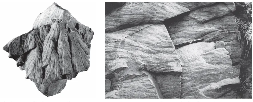
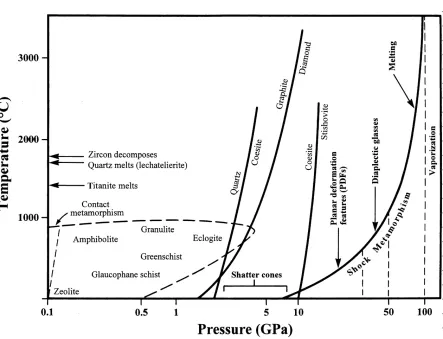
The second structure we will investigate is a shock metamorphic feature known as a shatter-cone. This is a physical structure which is formed under a relatively small range of pressures, and the formation of which is strongly associated with impact events [31]. To put it in plain language, as far as we know, a meteorite impact is the only natural process by which a shatter-cone will form. Shatter shatter-cones are almost entirely unique as a geologic object being the only shock deformation feature which is both distinctive to shock morphology and easily visible to an unaided eye. Ranging in size from a few centimetres to many metres [30, 55], these structures share a number of visual elements that are useful for identifying them, visually.

Shatter-cones are fluted quasi-conical structures, consisting of a curved surface with stri-ations (elongated traces with a preferred direction) which originate from a point along the shatter-cone surface and radiate outwards at small angles, with the striations ranging from 10µm to a few millimetres depending on the grain size of the rock[56]. They form in all types of rocks generally along pre-existing fracture planes, although the level of inhomogeneities within the rock structure may affect the formation of shatter-cones and typically result in par-tial cone formation aligned to the direction of impact. While typical, the underlying rock type will cause the formation of complete cones, as well as “fractal like” multiple nested “horse tail” structures and multi-directional shatter-cones where the cones are aligned 180 deg apart in direction, next to one another. (See figure 3.3b)

(26)

pres-3.2. Shatter-Cones 13

sures greater than 10 GPa while lower pressures 1-5GPa tend to produce features that are less differentiable from features causes by tectonic or volcanic processes.[31] (See figure 3.4 for a comparison of possible metamorphic processes.)

(a) A 30m Shatter-Cone from the Sud-bury impact site

(b) Hand Sized Inverted Shatter Cone from the Steinheim impact structure.

(27)

14 Chapter3. GeologicalFeatures

(28)

Chapter 4 Feature Extraction

4.1 Teaching a Computer To “See”

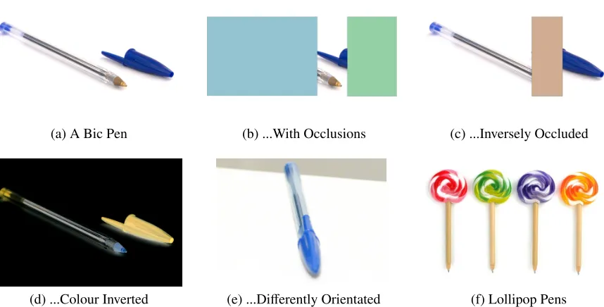
For most humans the act of seeing is not something that requires self-understanding, analysis or even conscious thought. To almost everyone seeing is such an intuitive an act that we are rarely aware as to the mechanisms that allow us to see. Imagine a pen sitting on a desk. Now ask yourself: “How do I know that this thing in my visual field is a pen?” What is its quintessential pen-ness? Perhaps it is the long thin shape, or the blue colour, or a uniquely recognizable feature such as it’s ball point nib. Perhaps it is a combination of features that make it recognizable. All of these suppositions are entirely reasonable assumptions... but are they correct?

If we examine the 6 different images of pens shown in Figure 4.1 we see that despite the wide variation in the configuration and appearance of the various pens, our ability to recognize each object as a pen is almost immediate. Figure 4.1a is the object as a whole, and yet, even when we occlude alternative sections of the pen in figures 4.1b and 4.1c we are still able to identify it as a pen despite no single piece of the image being duplicated. Likewise most people have little difficulty when we change the colour information as in 4.1d or the effect of foreshortening its shape by changing the pen’s orientation as in 4.1e. Finally if you look at the pens in figure 4.1f you will find that to identify the object as a pen, most of the visual information must be discarded in favour of a small portion (the ballpoint nibs on the end) in order to identify the object as a pen.

This ability to identify objects is, in and of itself, a difficult challenge if we wish for a computer to “see” an object, and yet even in the previous example, we have simplified a number of details in the way our visual system operates . How do we know where in our visual field the pen is? Is it large and far away? Is it small and close up? What delineates the end of the table and the beginning of the pen? How do we identify the nib, the body and the cap of different pens, even though they may look quite different from one pen to the next. Would you be able to identify the nib of a pen if one were placed in front of you without any context? How is it you know the size of the pen in figure 4.1a when you lack stereoscopic clues, and there are no other visual cues to reference it against?

As you may begin to appreciate, the “simple” act of seeing something is quite far from sim-ple. The human visual system is enormously sophisticated, and seeing is a complex, involved,

(29)

16 Chapter4. FeatureExtraction

(a) A Bic Pen (b) ...With Occlusions (c) ...Inversely Occluded

(d) ...Colour Inverted (e) ...Differently Orientated (f) Lollipop Pens

Figure 4.1: Despite a wide variation in visual information, humans are able to easily identify a pen, despite the fact that much of the visual information might be conflicting as seen in Figure 4.1f

and multi-level process that is the product of a phenomenal amount of neural processing by the human brain. It involves specialized neurological structures which have evolved to process and make sense of a busy and constantly changing visual field. It sets before the field of computer vision a complex model of what must be accomplished if a computer is to see. In order to allow a computer to see it must either mimic human processes to a certain degree, or develop computer specific ones that perform similar functions.

The first step in working with computer vision, is to establish a method by which various elements within an image can be described, and identified in a useful way. An image stored on a computer is in many ways analogous to a just seen image on the human eye. In the eye, the stimulation of rods and cones changes the rate of fire of the attached neurons allowing for the differentiation of colour and brightness at each location. In the computer an image is stored as a matrix of values, which represents the intensities of colours at each pixel. While this format is useful for the reproduction and display of an image, it does not provide context for what is contained within the image.

(30)

4.2. SIFT 17

It is this ability to create a series of visual words that must be mimicked in order to allow a computer to identify key objects within an image. In Computer Science these words are referred to as image features. These image features range from representations of a single pixel and its immediate neighbourhood, to a description of the image as a whole. They can describe a collection of key points or key regions, or the relationships between those points and regions. Each one will offer a description that can be analyzed, classified, and identified by an algorithm. Each of these words allows for the creation of a bag of visual descriptions for elements within an image.

Below is a brief overview of the features we used in our work.

4.2 SIFT

Scale-invariant feature transform(SIFT) features are a commonly used computer vision feature first published by Professor David Lowe from the University of British Columbia in 1999 [42]. The SIFT feature has become popular in the field of computer vision as a robust and useful feature. Part of the utility of the SIFT feature comes from the fact that it is formally invariant to translation, rotation, and zoom of an image. It has proven to be resistant to noise, blurring, and contrast changes, as well as having utility despite image deformations and affine transformations.

Each SIFT keypoint is a description of a given point on the image and its immediate neighbourhood. Each descriptor depends on 4 key variables: the horizontal position of the neighbourhood centre (x), the vertical position of the neighbourhood centre (y), the keypoint’s scale-space (σ), and the neighbourhood’s dominant gradient orientation (θ). These variables constitute the SIFT frame which describes the keypoint’s location scale and orientation. The feature’s descriptor encodes the surrounding neighbourhood gradient information (what Lowe named thekeypoint descriptor) into a 128-dimensional vector which can then be compared to similarly described points [43].

In his description of his method, Lowe identifies a 4 stage approach to creating the SIFT descriptor:

1. Scale-Space Extrema Detection 2. Accurate Keypoint Localization 3. Orientation Assignment

4. Keypoint Descriptor

This process can be further divided into 8 distinct algorithmic steps as seen in Table 4.1. Steps 1-3 correspond to Lowe’s scale-space extrema detection stage. Steps 4-6 correspond to the accurate keypoint localization stage and steps 7 & 8 correspond to the orientation assignment and keypoint descriptor stages respectively.

The first step to Lowe’s method is done to make the SIFT descriptor invariant to scale. This is done with a cascade of increasingly blurred images created by convolving the original imagel(x,y) with a variable-scale Gaussian filterG(x,y, σ) where the scale spaceL(x,y, σ) is described by the function:

(31)

Stage Description

1 Compute the Gaussian scale space 2 Compute the Difference of Gaussians 3 Find candidate keypoints

4 Refine candidate keypoints with sub-pixel precision 5 Filter noise unstable keypoints

6 Filter edge unstable keypoints

7 Assign an Orientation to each keypoint 8 Build the keypoint descriptor

Table 4.1: Sift descriptor Algorithm steps. (Adapted from Otero and Delbracio [50].)

This cascade of images is divided into octaves where each octave represent a doubling of the termσand each octave is itself divided intosintervals such thatk= 21/s_.with _s+_{3 images}

produced for each octave. For each octave the the sampling distance (δ) is also doubled. The resultant scale-space can be seen in figure 4.2.

Figure 4.2: A representation of a standard scale space where each dot represents an interval image vos Where o is the image’s octave and s is the interval. The dots in red represent the

images covering the whole octave while the dots in grey are used in extrema detection.

The second stage is the calculation of the Difference of Gaussian (DoG) scale-space. Lowe suggests that this step is necessary for true scale invariance by approximating the normalized Laplacianσ2∆_{[43]. The Di}ff_{erence of Gaussian scale-space is calculated by subtracting}

adja-cent blurred images in each octave. Thus the DoG image,D(x,y, σ) is calculated by:

D(x,y, σ)=(G(x,y,kσ)−G(x,y, σ))∗l(x,y)

=G(x,y,kσ)∗l(x,y)−G(x,y, σ)∗l(x,y)

= L(x,y,kσ)−L(x,y, σ)

(32)

4.2. SIFT 19

Figure 4.3: A representation of the Difference of Gaussian(DoG) scale space where each dot represents an interval image,wo

s Where,ois the image’s octave andsis the interval. The dots

in red represent the images covering the whole octave while the dots in grey supplementary images used for the extraction of candidate key points.

After establishing a DoG scale-space, keypoints are extracted by finding the continuous 3D extrema of the DoG scale-space. Practically speaking this must be done in two steps because of the discrete nature of the DoG scale-space. The first step detects the discrete extrema by comparing each pixel with its 26 neighbours, 8 neighbours within the image and the 9 corre-sponding pixels in the interval image above and below (see figure 4.4.)

Using a discrete method of detecting extrema on a continuous function causes intrinsic inac-curacy leads to unstable detections, and a susceptibility to noise. While Lowe’s original method did not have an interpolation step, Mathew Brown suggested a method of obtaining sub-pixel accuracy using a second order Taylor expansion to approximate the underlying function[5].

Figure 4.4: Extracting candidate keypoints by finding 3D Extrema.

The final step in determining accurate keypoint localization is to reject inherently unstable keypoints. Two main classes of keypoints are rejected at this point. Keypoints in areas of low contrast being inherently unstable, are eliminated using a threshold and keypoints along edges which may be translation invariant along that edge are eliminated using a Hessian Matrix.

(33)

Figure 4.5: The sum of the pixels within rectangleD(1,2,3,4) of the original image can be

com-puted using the four corner points within the integral image. Point 1 gives the area of A, Point 2 the area of A+B, Point 3 the area of A+C, Point 4 the area of A+B+C+D. This means we can find the value for area D. (D=1+4−(2+3))

dominant gradient angleθis found an keypoint descriptor is generated by using a 16x16 ma-trix is normalized aboutθ. The dominant gradient of each element of this matrix is assigned to one of 8 orientations which are grouped in 4x4 regions. This generates a 4x4x8 matrix which forms a 128 dimension description vector for the keypoint.

4.3 Haar Like Features

Haar like features are a name given to an image feature first described by Paul Viola and Michael Jones in their 2001 paper,Rapid Object Detection using a Boosted Cascade of Simple Features[63]. Haar like features are an intensity based feature that utilize an additive method for comparing adjacent rectangles. Viola and Jones’ method also adds a cascade of features, which helps reduce the computational complexity while maximizing accuracy. The result of this combination produced a comparatively accurate detection algorithm which was much more efficient than previous work (Viola and Jones claimed their algorithm was 15 times faster than previous work.)

The Viola/Jones implementation of Haar like features begins with the creation of an image representation the authors called anintegral image. The integral image is a 2D vector where the value at (x,y) in the integral image (ii) is a sum of all of the pixel intensities in the image to be processed to the left and above the same point on the original imagei(x0,_y0_).

ii(x,y)= X

x0_≤_x_,_y0_≤_y

i(x0,y0)

The integral image is created in order to allow for the rapid summation of image intensities. In figure 4.5 the sum of image intensities within a given rectangle (ii1,ii2,ii3,ii4) can be

(34)

4.4. EOG 21

the sum of the intensities of the area above and left, we see that:

the point= is the sum of intensities of the area represented by: ii1 = A

ii2 = A+B ii3 = A+C

ii4 = A+B+C+D

From this we can see that the area of D is equal to:

D= (ii1+ii4)−(ii2+ii3)

This ability to quickly compare the intensity of image areas allows for the creation of compu-tationally cheap features. Viola and Jones used the differences in intensities between adjacent squares within a 24x24 pixel subsection of an image in order to create weak classifiers (see figure 4.6a.)

(a) An example of features used by Viola and Jones for face detection

(b) An extended feature set

Figure 4.6: Haar like features created by difference combinations of additive and subtractive non-overlapping intensity area summations.

4.4 EOG

(35)

Freeman and Roth used derivative operators dx and dy to generate their gradients with arctan(dx,dy) corresponding to the gradient direction and pdx2+_dy2_{being the gradient}

con-trast. They divided the gradients into one of 36 bins and then blurred and normalized the results to create a descriptor.

In modern algorithmic implementations of EOGs a variety of 2D filters may be used such as sobel operators to determine the gradient in a number of different directions. The histogram bins have been simplified to 5 traditionally consisting of 4 directional gradients (N-S, E-W, NE-SW, NW-SE) and one unidirectional gradient (see figure 4.7.) To make these histograms a useful image feature, many implementations will calculate these localized gradients over a variety of image window scales, to allow for a larger vocabulary of words.

-1 -2 -1

0 0 0

1 2 1

(a) Horizontal

-1 0 1

-2 0 2

-1 0 1

(b) Vertical

2 2 -1

2 -1 -1

-1 -1 -1

(c) NW-SE Diagonal

-1 2 2

-1 -1 -2

-1 -1 -1

(d) NE-SW Diagonal

-1 0 1

0 0 0

1 0 -1

(e) Non-Directional

Figure 4.7: 4 Directional Sobel operators and one non directional one too.

Figure 4.8: A modern Edge Orientation Gradient

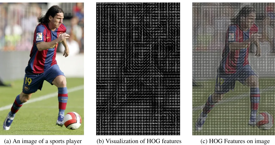
4.5 HOG

Histogram of Oriented Gradients (HOG) was developed as a method of edge detection for the purpose of detecting people in images. First devised in 2005 by Navneet Dalal and Bill Triggs, HOG is similar to SIFT, but rather than focusing on key points, HOG is computed in dense grids at a single scale without assigning an orientation[19]. Because it is calculated in a grid, the HOG feature takes advantage of overlapping sub windows to normalize the local contrast (unlike EOG.)

(36)

4.5. HOG 23

(a) An image of a sports player (b) Visualization of HOG features (c) HOG Features on image

Figure 4.9: Histogram of Oriented Gradients were first used to describe the positions of a body for the purpose of identifying that it was a person. Image 4.9c above shows the corresponding gradients from the HOG results in 4.9b of the sports player image in 4.9a

Dalal and Triggs outlined a 6 step process for their use of HOGs (See Figure 4.10.) The Process begins by normalizing the gamma/colour space, Dalal and Triggs reported that they were able to use this process on both grayscale and colour images with the colour information providing slightly better results overall. The second step is it to calculate the gradient of the image, using a gradient filter. In the case of colour images, each colour channel is calculated separately. Dalal and Triggs list four variations of gradient filters they tried, Sobel operators, (as seen in fig.4.7) in addition to three 1-D derivative filters: uncentered [−1,1], centred [−1,0,1], and cubic corrected [−1,−8,0,8,1]. Dalal and Triggs reported that the best results came from the 1-D centred filter and its transpose, but only marginally so and while they speculate on reasons, it is not clear that this is universally true.

In the third step, Dalal and Triggs divide the image up into blocks of cells, each cell con-taining a similar number of pixels, each of whom votes for an orientation bin based on the gradient magnitude at its location. The orientation bins are evenly spaced over the whole rota-tional range (0◦₋₁₈₀◦_for

unsignedgradients and 0◦₋₃₆₀◦_for

signedgradients.) These votes are then interpolated bilinearly between neighbouring orientation and position bins. The cells are made up of a block of pixels arranged spacially in either rectangular or a radial orientation. Each of these cells is then assigned to a series of overlapping blocks such that each cell belongs to a number of adjacent blocks. (i.e. a stride of 1₂ of the block size ensures that every non edge cell belonged to 4 adjacent blocks. This overlapping nature is imperative for the Dalal and Triggs next step.

(37)

image blocks, they ensure that each region is normalized with a number of surrounding blocks. Dalal and Triggs explored four different methods for block normalization.

Lethbe the non-normalized vector of histograms in a given block.

khkk is its k-norm fork ={1,2}

ande= some small constant.

The normalization factors tried were the following:

L2-norm: f = _q v

kvk2 2+e2

L2-hys: L2-norm withvmaxlimited to 0.2 and renormalized.

L1-norm: f = v

(kvk₁+e)

L1-sqrt: f =

r

v (kvk₁+e)

In their experiments, Dalal and Triggs found the L2-Hys, L2-norm, and L1-sqrt schemes provide similar performance, while the L1-norm provides slightly less reliable performance; however, all four methods showed very significant improvement over the non-normalized data. After performing this normalization, the feature vector is created by collecting each cell from each block of the detection window to create a feature vector.

Figure 4.10: Dalal and Triggs described a six step process in their 2005 paper.[19]

4.6 Hough Transforms

(38)

4.6. HoughTransforms 25

(a) Rho Theta Notation (b) A Point described in Polar Space (c) Points on a line

Figure 4.11: In 4.11a a point in space can be described by it’s distance from, and rotation about the origin. 4.11b is that point as described in Polar Space. 4.11c shows the polar representation along a straight line in Cartesian Space.

parametrized to find specific shapes, and a more general one that is more commonly used as an image descriptor. Since the first incarnation of this algorithm requires a paramiterization of the desired shape, it is generally reserved for, regular curves such as lines, circles, ellipses etc. One of the key strengths of the Hough transform technique is that it is tolerant of gaps in feature boundary descriptions and is relatively unaffected by image noise.

The Hough Transform takes its name from Paul Hough, who rst described the fundamental principles in a 1960 patent for his work in bubble chambers at the U.S. Atomic Energy Com-mission. [7]. Hough’s methods were improved upon and the algorithm optimized for image detection by Duda and Hart in their 1971 paper, Use of the Hough Transformation to Detect Lines and Curves in Pictures[23]. One of the key differences in the work of Duda and Hart, is their use of rho-theta notation. Traditionally image notation is given in Cartesian Space, thus a pixel will be denoted as the combination of the horizontal and vertical offset from the origin. (x,y) and a line can be denoted as a function of a series of pixels (x1,y1),(x2,y2), ...,(xn,yn) if

the line is a regular curve, it can be described using two parameters,{m,b}where m is the slope and b is an offset. Thus any regular curve can be written as:

y=mx+b (4.1)

The problem with the use of Cartesian Space was that m could be infinity. Duda and Hart’s use of rho-theta notation prevents this from happening. Duda and Hart translated point descriptions from Cartesian Space to Polar Space thus preventingm=∞. In figure 4.11a we can see that a pixel in Cartesian Space can also be described as a function of its distance from, and rotation about, the origin. Thus we can write it as:

y=

−cosθ

sinθ x+ _r sinθ (4.2)

This can then be arranged into polar coordinates:

r = xcosθ+ysinθ (4.3)

this means that for any given pixel (x1,y1) a representation in polar space can be given as a

function of all of the lines passing through that point as:(see figure 4.11b for the curve produced byx1 =8 andy1 =6)

(39)

If the same operation is performed for all the points in an image it will produce a series of sinusoidal curves in polar space. If the curves of two different points intersect in the plane

θ − r, we can say those points are along the same cartesian line. For instance, following expanding on the example above if by plotting two more points along a line: (x2 = 9,y2 = 4

andx3 =12,y3= 3, we get the result shown in figure 4.11c.

We can see from equation (4.2) and equation (4.1) that this intersection is comes from the parametersmandbin cartesian space equate to a function ofrandθin polar space.

m=

−cosθ

sinθ (4.5) and b= r sinθ (4.6)

The fact that the curves of points on a line intersect allows for powerful tools of analysis. By assigning a value to each pixel along the curves in Polar Space, a cumulative energy value can be assigned to points and an energy map produced, whereby those points in r, θ space with the highest values correspond to the most dominant linear feature. Likewise lines which are not quite linear but fall near a line can be grouped by counting all values within a given neighbourhood in Polar Space. Likewise since parallel lines in cartesian space have the same slope(m) equation (4.5) suggests that parallel lines will be located at peaks same point along theθaxis in polar space.

Since the Hough Transform is a translation between Cartesian and Polar Spaces, performing a translation on an image would result in a curve for every pixel, rendering the results pretty much meaningless. In order to maximize the value of the Hough transform, it is beneficial to maximize the information contained in the pixels entered into the transform. Since edges generally contain the largest amount of information, an edge detection algorithm (such as the canny edge detector) is generally used to produce a binary value image,which is then passed into the hough transform.

To use a Hough Transform as a general image descriptor for a machine learning program, hough peaks are calculated and labeled biased on a threshold value. Those peaks are then clustered either in two dimensions or one (keeping in mind that (4.5) suggest that clustering along theθaccess will give you an indication of parallel lines.) These clusters are then used to create an image descriptor.

4.7 Intensity and Colour Histograms

(40)

4.8. EdgeDensity 27

(a) Identical Intensity Histograms for dissimilar images

(b) Susceptibility of Intensity His-tograms to Lighting Changes

(c) Rock VS. Regolith

Figure 4.12: With out careful application, intensity histograms can exhibit a number of different weaknesses. Properly applied however they form a useful tool.

very susceptible to lighting changes, and so the same image taken with different lighting may create vastly different histograms as well (see figure 4.12b.)

Despite these obvious weaknesses intensity histograms can still be useful within their in-trinsic limitations. Histograms offer a computationally low cost method of describing an image patch, and as can be seen in figure 4.12c, they seem to be useful in the case of our work in par-ticular because of the relatively homogenous colouring of large parts of extraterrestrial regolith. This same attribute also offers promise in its ability to help differentiate between different types of rocks as well.

4.8 Edge Density

Edge Density is an image descriptor which as its name implies calculates the density of edge pixels located within an image or image sub-window. The edge density is found by using a binary edge detection algorithm such as a canny edge detector and then the density of the edges is calculated using the formula:

f = 1 ar

x2 X

x=x1

y2 X

y=y1

e(x,y) (4.7)

where:

ar= (x2−x1+1)(y2−y1+1) (4.8)

Wheree(x,y) is the detected edge image of a sub-windowi(x,y) of the original imagei. ar is

(41)

Chapter 5 Machine Learning Algorithms

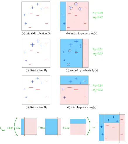
Once image features have been extracted from an image, there must be a way of giving those features meaning. Image features are in essence a group of words which can be used to describ-ing what an image contains, but as yet we do not have the vocabulary to describe the contents of an image. For a human being, the development of linguistic context makes up a large part of our early years. Through trial and error and experimentation a child learns to classify the things they see into meaningful groupings based on contextual clues. The contextual and struc-tural rules the child develops are associated with the signals arriving from sensory organs, and through repeated experience allows for a system of comparison which allows a child to classify novel objects from similarities to known things.

This process of learning through known examples is referred to as “concept learning” in psychology [6]. In computer science this is known as “supervised learning” because an outside expert is required to “supervise” the learning process by providing a training set for the com-puter to learn on. It is this process of supervised learning that is used to create a language to describe features within images.

5.1 What is Machine Learning?

In the most general sense, machine learning can be thought of as a computer learning from past experience, or in the words of Tom Mitchell,“A computer program is said to learn from expe-rienceE with respect to some class of tasksT and performance measureP, if its performance at tasks inT, as measured byP, improves with experienceE[45].”

Machine learning differs from what might traditionally be thought of as programming, because the computer is not given explicitly coded instructions of how to accomplish a task, rather it is given a set of rules by which it can evaluate its performance(Pin Tom’s words) and a way of revising it’s method of performing a task (T). There are a wide variety of learning strategies, but they generally fall into three main categories.

Supervised Learning Supervised learning, as we alluded to above, is when an algorithm is given a set of objects which have previously been identified, and are given to a learning algo-rithm to evaluate. Once the algoalgo-rithm has classified the images, the results are evaluated and some form of refinement is applied, either from a weighting function based on the identified,

Geological Object Recognition in Extraterrestrial Environments

Scholarship@Western

Scholarship@Western

Geological Object Recognition in Extraterrestrial Environments

Geological Object Recognition in Extraterrestrial Environments

GEOLOGICAL OBJECT RECOGNITION IN EXTRATERRESTRIAL

ENVIRONMENTS

(Thesis format: Monograph)

by

Greg Elfers

Graduate Program in Computer Science

A thesis submitted in partial fulfillment

of the requirements for the degree of

Masters of Science

The School of Graduate and Postdoctoral Studies

The University of Western Ontario

London, Ontario, Canada

c

Acknowlegements

Abstract

Contents

List of Figures

List of Tables

Chapter 1

Introduction

1.1

Motivation

1.2

Scope of our investigation

1.3

Approach

1.3.1

Program Workflow

1.4

Outline

Chapter 2

Previous Work

2.1

SLAM

2.2

Rock Detection

2.3

Material Identification

2.4

OASIS, AEGIS and GESTALT

Chapter 3

Geological Features

Rock,

n.

3.1

Outcrops

3.2

Shatter-Cones

Chapter 4

Feature Extraction

4.1

Teaching a Computer To “See”

4.2

SIFT

4.3

Haar Like Features

4.4

EOG

4.5

HOG

4.6

Hough Transforms

4.7

Intensity and Colour Histograms

4.8

Edge Density

Chapter 5

Machine Learning Algorithms

5.1

What is Machine Learning?