GEOPHYSICAL PROSPECTION OF IRON-TITANIUM OXIDE (ILMENITE) USING MAGNETIC METHOD IN MAGAONI, KWALE COUNTY, KENYA.
ODUOR GEORGE OTIENO (B.ED SC).
I56/CE/25986/2011.
A thesis submitted in partial fulfilment of the requirements for the award of the degree of Master of Science (Physics) in the School of Pure and Applied Sciences of Kenyatta University.
ii
iii
iv
ACKNOWLEDGEMENTS
I am so thankful to the Almighty God for the good health, strength and financial capacity
towards the successful completion of my Msc. program.
My strong credit goes to my research supervisors, Dr. W.J. Ambusso and Dr. J.G. Githiri for
their unequalled assistance and guidance. I also thank the Chairman Physics Department,
Kenyatta University, and the entire physics department lecturers and laboratory technicians for
their support during my studies.
I am grateful to my dear wife Mrs. Donata Oduor and my daughter Eve and son Lawi for their
support and understanding during my Msc program. I would also like to recognize the
all-important prayers and moral support from my mum, Mrs. Biliah Otieno and all the other family
members during my studies.
I will not forget the overwhelming support received from Sheikh Khalifa High School
v
TABLE OF CONTENTS
Table of Contents
DECLARATION... ii
DEDICATION... iii
ACKNOWLEDGEMENTS ... iv
TABLE OF CONTENTS... vi
LIST OF TABLES ... ix
LIST OF FIGURES ... x
LIST OF ABBREVIATIONS ... xii
ABSTRACT ... xiii
CHAPTER ONE
INTRODUCTION... 11.1 Background to the study ... 1
1.2 Study area...1
1.3 Geology of Magaoni………..………3
1.4 Statement of research problem………...5
1.5 Objectives of the research project ...6
1.5.1 Main objective ...6
1.5.2 Specific objectives ...6
vi CHAPTER TWO
LITERATURE REVIEW ...8
2.1 Introduction……...8
2.2 Prospection of strong magnetic mineral ores…………...8
2.3 Prospection of weak and nonmagnetic mineral ores…...9
2.4 Ilmenite prospection………...……9
2.5 Ilmenite prospection in Kwale County………...…….10
CHAPTER THREE THEORETICAL BACKGROUND ...12
3.1 Introduction ...123.2 The Geomagnetic field ...14
3.2.1 Geomagnetic field elements…………. ...18
3.2.2 Rock magnetism...19
3.3 Ground Magnetic method………...……….21
3.4 Magnetic method in exploration………..21
CHAPTER FOUR MATERIALS AND METHODS ... 23
vii
4.1.1 Introduction ... 23
4.2 Field equipment...24
4.2.1 Global positioning system...24
4.2.2 Flux Gate Magnetometer ...24
4.3 Field measurements ... 25
4.4 Magnetic data correction ... 25
4.4.1 Diurnal variations corrections ...25
4.4.2 Geomagnetic field correction ... 27
4.5 Data enhancement………27
4.5.1 Trend analysis………...27
4.5.2 Reduction to the pole………...……….30
4.5.3 Vertical and horizontal derivative……….30
4.5.4 Euler deconvolution………..…30
4.6 Chemical analysis of samples………...31
4.6.1 Titanium………...….31
4.6.2 Iron (III) Oxide………...………..32
4.6.3 Energy Dispersive X-Ray Fluorescence Spectroscopy……….……32
CHAPTER FIVE RESULTS AND DISCUSSION………...35
5.1 Introduction ...35
5.2Interpretation of Magaoni magnetic anomaly map ...36
viii
5.4 Interpretation of chemical analysis results………...………45
5.5 Discussion of magnetic data………50
5.6 Discussion of chemical analysis results………..………...51
CHAPTER SIX CONCLUSIONS AND RECOMMENDATIONS ... 53
6.1 Introduction ...53
6.2 Conclusions ... 53
6.3 Recommendations ... 54
REFERENCES ... 55
APPENDIX I: BS DIURNAL CURVES………...58
APPENDIX II: PROFILE GRAPHS………...…………..64
ix
LIST OF TABLES
Table 3.1: Basic patterns of alignment of atomic magnetic moments 21
Table 5.1: Analysis result for sample SS13 47
Table 5.2: Analysis result for sample SS16 48
Table 5.3: Analysis result for sample SS20 48
Table 5.4: Analysis result for sample SS21 49
Table 5.5: Analysis result for sample SS24 49
x
LIST OF FIGURES
Figure 1.1: Location map of Magaoni 2
Figure 1.2: Geological map of Southern Kenyan coast. 3
Figure 3.1: Earth’s magnetic field vector diagram 16
Figure 4.1: Diurnal curve for day seven of the study 26
Figure 4.1a: Graph of profile AA’ with regional 29
Figure 4.2b: Graph of profile AA’ without regional 29
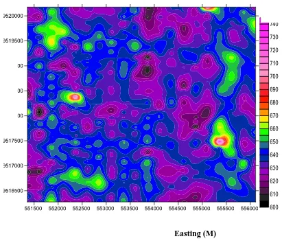
Figure 5.1: Magnetic Intensity colour contour map of the study area 36
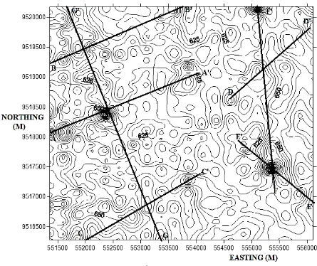
Figure 5.2: Magnetic Intensity contour map with profiles for the study area 37
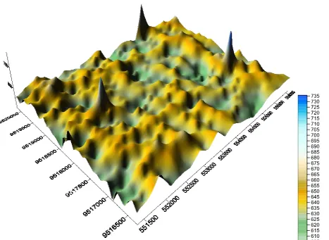
Figure 5.3: 3D Magnetic Anomaly map for the study area 38
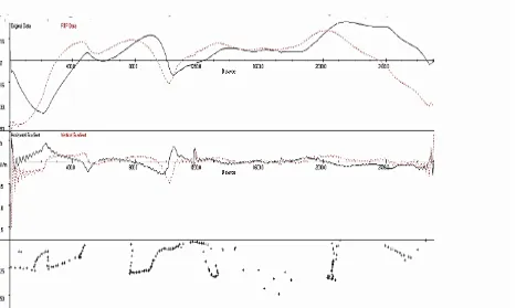
Figure 5.4: Euler depth solutions along profile AA’ 40
Figure 5.5: Euler depth solutions along profile BB’ 41
Figure 5.6: Euler depth solutions along profile CC’ 42
Figure 5.7:Euler depth solutions along profile DD’ 42
Figure 5.8: Euler depth solutions along profile EE’ 43
Figure 5.9: Euler depth solutions along profile FF’ 44
xi
LIST OF ABBREVIATIONS AND ACRONYMS
2D Two-Dimension
AC Alternating Current
BH Horizontal component of geomagnetic field
BS Base Station
BT Total magnetic intensity vector
Bz Vertical component of geomagnetic field
C.V Corrected Value
DC Diurnal Correction.
EDXF Energy DispersiveX-Ray Fluorescence
GPSGlobal Positioning System
IGRF International Geomagnetic Reference Frame
M.V Measured Value
RTP Reduced to the Pole
USGS United States Geophysical Survey
xii
ABSTRACT
1
CHAPTER ONE
INTRODUCTION
1.1
Background to the study
Ilmenite is iron-titanium oxide (Fe.TiO3) mineral which is iron-black or steel-grey in colour. It is
mineral sand found either on the primary rock or sedimentary deposits along shorelines or
several kilometres off the shoreline. Ilmenite from sedimentary deposits is the commonly
explored due to the easy accessibility and low mining costs. Most mineral sand deposits being
mined today were formed during the Holocene and Pleistocene period but some date back to
Eocene (Shepherd, 1987). It is one of the 60 minerals in which titanium occurs, just like rutile,
anatase, zircon, brookite etc. It is weakly magnetic but produce observable magnetic responses.
Ilmenite is opaque with no cleavage; it has metallic or submetallic lustre and its specific gravity
ranging between 4.7 to 4.8. Ilmenite crystallizes in the trigonal system; the ilmenite structure is
an ordered derivative of the corundum structure. It is one of the heavy minerals that occur as
separate 0.1 to 1.0 mm grains, containing locally few silicate inclusions, magnetite occur as
smaller grains around ilmenite lamella (Jokinen, 1999).
1.2 Study area.
The study area, Magaoni is located about 50 km south of Mombasa, off Ukunda-Lunga Lunga
road, the area lies within the coordinates 40 22’S 390 21’E and 40 25’S 39 230E(Figure 1.1).
Ilmenite (Iron-Titanium oxide) and other heavy minerals bearing areas was explored and mapped
by Tiomin Company in Maumba and Nguluku, a few kilometres from Magaoni, Kwale County.
2
Magaoni area and the mining sites being in Kwale region have similar geological setting and
was therefore considered likely that heavy minerals, especially ilmenite and rutile are present in
the area. The study was conducted in this area to establish the extent of ilmenite distribution in
Kwale County.
3 1.3 Geology of Magaoni
The area lies within the Magarini sands formation which forms a belt of low hills parallel to the
coast. The mineralisation of Kwale region lies within stratified Aeolian sands of the Magarini
formation and consists mainly sand, with silicate and ilmenite as a dominant minerals, rutile and
zircon, deposited in dunes as shown in figure 1.2. The deposit forms a belt of low hill running
parallel to the coast. The area contains a silt fraction varying from 15 to 30 %. (Miller, 1952).
4
The sands were deposited by wind action as coastal dunes after conditions of intense erosion
causing heavy minerals, mainly ilmenite, rutile and zircon to be locally concentrated (Miller,
1952). Erosion prevailed during the tertiary until the upper Pliocene, when tectonic reactivation
resulted in increased erosion from structural highs (Miller, 1952). Fluviatile pebble beds, gravels
and sands of the Magarini formation were deposited on down-faulted and eroded Jurassic and
Duruma sediments. After a regression during the lowest Pleistocene, dunes which form the bulk
of the Magarini formation were blown-up. The rocks exposed consist of sediments ranging in
age from Permo-Carboniferous deposition. Igneous and pyroclastic are confined to Jombo Hill,
an alkaline intrusion, and associated satellite vent agglomerates and dykes (Miller, 1952).
The Duruma Sandstone Series, which is in the Kenyan correlative of the Karroo System of South
and Central Africa, consists of grits, sandstones and shales that have yielded Permain and
Triassic fossils, although it is possible that the series ranges down-wards to Upper Carboniferous
and upwards to the Lower Jurassic. The series is divisible into three broad lithological units with
coarse sandstones and grits at the top and bottom of the succession, and a finer sandstones and
shales in the middle. For the most part the beds were deposited under lacustrine or sub-aerial
conditions, the material having been derived from the Basement System rocks further, west. A
marine intercalation in the lower part of the succession is known from evidence obtained in a
deep borehole drilled near Maji-ya-Chumvi. General stratigraphic sequence is composed of
brown sand at the surface followed by orange or reddish sand becoming more beige or pinkish at
5
The generally close relationship of continental rifting with alkaline magmatism is documented at
the southern Kenyan coast by the Jombo-Mrima alkaline complex, tentatively dated as
cretaceous. The major alkaline intrusion of Jombo Hill and Dzirihini, consist of nepheline
syenite surrounded by mafic alkaline rocks (malignites, jolites, melfeigite, juvite and foyaites).
Associated with them are the carbonatite complexes forming Mrima Hill as well as agglomerate
vents, kimberlite diatremes and minor volcanic vents. The geology of the Kenyan south coast is
a major factor in the occurrence of heavy mineral sands. The heavy mineral sands occur in
various parts of the coast in almost similar geological environments. Geochemically, mineral
sand deposits contain ilmenite, rutile, zirconium as well as other minerals and trace elements that
could be of radioactive nature, such as thorium. (Miller, 1952).
1.4 Statement of research problem . Magaoni area is located on the southern part of Kwale County, Kenya. The area is significant
due to the presence of sedimentary deposits associated with heavy minerals. Magaoni area is
close Maumba and Nguluku, which contain economically viable concentration of heavy minerals
such as ilmenite and zircon, as mapped by Tiomin Company using mineral assemblage method.
Due to the increase in demand for titanium and titanium pigment in industrial processes
worldwide and the need to improve the living standards of the locals and the economy of the country, it’s therefore necessary for research to be undertaken in this area, to increase the number
6
This study used ground magnetic method to determine the extent of Ilmenite deposit in Kwale
County because the method is quite affordable and can be used to cover a large area. Ilmenite is
a magnetic mineral and therefore magnetic method was the best geophysical technique for its
prospection. The study was done in order to give recommendation on the possibility of large
scale mineral sand exploration and eventual mining. This will supplement the tonnage of
Ilmenite being mined by Base Titanium Company, which will definitely attract investors to open
titanium processing Industries in the country. That will translate to more revenue to the country
and more job opportunities to the citizens.
1.5 Objectives of the research project
1.5.1 Main Objective
To determine the lateral extension of the iron-titanium oxide (ilmenite) deposits in Kwale
County through the application of ground magnetic method.
1.5.2 Specific Objectives
The specific objectives of this study were:
(i) To conduct a ground magnetic measurements in Magaoni area, Kwale County.
(ii)To carry out chemical analysis of randomly sampled surface soil samples to determine
7 1.6 Rationale of the study
The information of availability of ilmenite (iron titanium oxide) bearing sand is an important
reason for resource assessment. This can provide a possibility of a high profile large scale
prospection and mining of ilmenite, which will in turn encourage the creation of titanium
processing industries, which will mean more employment opportunities and economic
8
CHAPTER TWO
LITERATURE REVIEW
2.1 IntroductionMagnetic method is a geophysical survey technique that exploits the considerable differences in the magnetic properties of minerals with ultimate objective of characterising the Earth’s
sub-surface. The technique requires the acquisition of measurements of the amplitude of the magnetic
field at discrete points along survey lines distributed regularly throughout the mineral prospect
area. The technique has been used successfully in the prospection of weak, moderate and strong
magnetic minerals. The method has been used to directly and indirectly delineate the mineral ore
body in the prospect area.
2.2 Prospection of strong magnetic mineral ores
Magnetic method is considered the most reliable and cheap technique in the prospection of
magnetically strong minerals, this is because the method locates the ores. Areas with strong
magnetic minerals bearing rocks will give high and positive magnetic anomalies. Mineral ore
such as magnetite, gives high and positive magnetic anomaly during prospection because of it
being a strong magnetic mineral. For instance in Meru County, Kenya, magnetics was
successfully used to map out iron ore deposits (magnetite). The total magnetic field data acquired
from the study area, showed high magnetic signatures around magnetite bearing formations
(Mustafa, 2010).
In Central Java Indonesia, magnetic method was used to directly map magnetite bearing
9
high values of total magnetic field intensity and magnetic susceptibility respectively, indicating
presence of magnetite (Yulianto, 2002).
2.3 Prospection of weak and non-magnetic mineral ores
Magnetic method has also been used with great success in the exploration of weak and
non-magnetic minerals. The weak and non-non-magnetic signatures give very sharp non-magnetic contrast
which provides anomalies that can be used indirectly to locate the mineral ores. Example of
weak magnetic mineral ores is ilmenite, while for the non-magnetic are rutile, pyrite, and gold
among others. Ilmenite was explored and mapped using this technique in several countries, as
discussed in the next subtopic. In Hired Iran, magnetic method was used delineate host rocks of
gold ore which are non-magnetic. Based on the sharp magnetic contrast, magnetic method survey
revealed large anomalies. Further investigation with chemical analysis showed the source of the
anomalies was pyrrholite along with gold (Haidaria, 2009).
2.4 Ilmenite prospection
Ilmenite gives a weak but observable magnetic responses, it has a magnetic susceptibility whose
intensity allows the detection by magnetometers. The average value of magnetic susceptibility of
ilmenite is 0.0018 SI (Telford, et al., 1976). The host rocks of ilmenite, granite, granodiorite and
monazite have low magnetic susceptibility, creating a magnetic contrast which makes magnetic
method suitable for its prospection. The method can be more effective when combined with
either gravity method or radiometry or chemical analysis of samples from the study area
10
In Brazil, at the delta of the Paraiba do Sul River, north of the Rio de Jeneiro state, magnetic
method was used to prospect ilmenite. The magnetic survey was conducted to measure the Total
magnetic field of the earth using a magnetometer type GSM-19TG. The study was conducted
through profile NW – SE direction, traversed to the direction of advancement of an active
mining. The profiles were spaced 20m from one another with stations spaced 5m. In the 21
surveyed profiles, 955 measurements were performed. The analysed results showed consistence
with ilmenite. Kappa meter KT9 was used to measure magnetic susceptibility of samples of
ilmenite and it showed a mean value of 0.002 SI, which is within the range of ilmenite. In
Finland, at Loivusaarenneva and Kairineva, ilmenite deposits were mapped using magnetic
method. Therefore, ilmenite can be prospected by magnetic method since it is a predominant
carrier of magnetic signature just like other iron-titanium oxides. (Karkkainen, 1999a).
2.5 Ilmenite exploration in Kwale County
Exploration was done from 1997 by Tiomin Resource Inc. and three dunes were mapped out in
Maumba and Nguluku. The dunes were named, Central, South and North dunes, with high
concentration of ilmenite, rutile and zircon. The company used geological and geochemical
methods in the exploration, it involved drilling to get samples at different depths and locations.
The samples were taken to the laboratories for analysis of ilmenite, rutile and zircon ores.
Samples were screened and then subjected to a heavy mineral float/sink technique using heavy
liquids; tetra-bromo-ethane (TBE with a SG of 2.92-2.96 gcm-3). The resulting Heavy Mineral
Concentrate was then dried and weighed. The samples were then subjected to magnetic
separation using Carpco magnetic Capturing various magnetic nonmagnetic fractions which were
11
The XRF analysis was used to calculate by formula and ratios, the percentage of mineral species
that constitute the valuable and non-valuable Heavy Mineral. Several surface and auger sampling
spaced 10 km apart were completed across the width of the survey areas. Total Heavy Mineral
contents of the samples collected ranged from 1.8 % up to 14.6 %, ilmenite valued up to 10.6 %
and 0.94 % non-magnetic mineral including rutile and zircon. Central dune measures 2 km
length, 1.25 km width and average thickness of 29 m, 5.7 % Heavy Mineral Concentration. The
South dune is 4.5 km long, 600-800 m wide and average thickness of 19 m and 3.5 % HMC.
Finally, North dune extends 2 km in length, 500-1000m and 66 m thick and 2.1 % THM (Tiomin
12
CHAPTER THREE
THEORETICAL BACKGROUND
3.1 Introduction
The purpose of magnetic surveying is to identify and describe regions of the Earth’s crust that
have unusual (anomalous) magnetizations. In the realm of applied geophysics the anomalous
magnetizations might be associated with local mineralization that is potentially of commercial
interest, or they could be due to subsurface structures that have a bearing on the location of
geothermal heat source or even oil deposits. The magnetic method involves the measurement of the Earth’s magnetic field at predetermined points, correcting the measurements for known
changes and comparing the resultant value of the field with expected value at each measurement station. Magnetism, like gravity, is a potential field. Anomalies in the earth’s magnetic field are
caused by induced or remanent magnetism. Induced magnetic anomalies are the result of secondary magnetisation induced in a ferrous body by the earth’s magnetic field. The shape,
dimensions, and amplitude of an induced magnetic anomaly is a function of orientation,
geometry, size, depth, and magnetic susceptibility of the body as well as the intensity and inclination of the Earth’s magnetic field in the survey area (Merrill et al., 1996).
For exploration work, the Earth’s Main Field acts as the inducing magnetic field. This is a
relatively small portion of the observed magnetic field that is generated from magnetic sources
external to the earth. This field is believed to be produced by interactions of the Earth's
ionosphere with the solar wind. Hence, temporal variations associated with the external magnetic
field are correlated to solar activity. When describing temporal variations of the magnetic field, it
13
and source. There are three temporal variations: Secular Variations - These are long-term
(changes in the field that occur over years) variations in the main magnetic field that are
presumably caused by fluid motion in the Earth's Outer Core. Because these variations occur
slowly with respect to the time of completion of a typical exploration magnetic survey, these
variations will not complicate data reduction efforts (Doel and Cox, 1967).
Diurnal Variations - These are variations in the magnetic field that occur over the course of a day
and are related to variations in the Earth's external magnetic field. This variation can be on the
order of 20 to 30 nT per day and should be accounted for when conducting exploration magnetic
surveys. Magnetic Storms - Occasionally, magnetic activity in the ionosphere will abruptly
increase. The occurrence of such storms correlates with enhanced sunspot activity. The magnetic
field observed during such times is highly irregular and unpredictable, having amplitudes as
large as 1000 nT (Wright, 1981).
Exploration magnetic surveys should not be conducted during magnetic storms. This is because
the variations in the field that they can produce are large, rapid, and spatially varying. Therefore,
it is difficult to correct for them in acquired data. Magnetised materials produce magnetic field around themselves and if they are close to the Earth’s surface, their magnetic field combine with
the earth’s field. Magnetised matter contains a distribution of microscopic magnetic moments.
Magnetisation J is defined as the magnetic dipole moment per unit volume of the material.
Induced magnetisation JI is the component of magnetisation produced in response to an applied
14
magnetising field is removed and essentially unaffected by weak fields. Total magnetisation is
the vector sum of the induced and remanent magnetisation (Reeves, 1989).
J = JI + JR 3.1
For sufficiently weak fields, such as the geomagnetic field the, the induced magnetisation is approximately proportional to the applied field. The constant of proportionality is known as susceptibility, K, magnetic susceptibility is the measure of the degree to which a substance may be magnetised (Wasilewski, 1973). If the applied field is F.
JI = KF; J = KF + JR 3.2
The Koenisberger ratio (Q) is a convenient parameter for expressing the relative importance of remanent and induced magnetisation, it’s given by;
Q = JR / JI 3.3
3.2 The Geomagnetic field
This is the magnetic field of the earth, which can be measured at any part on the earth’s surface.
The magnetic field on the earth at a given place and time may be considered to consist of three
parts. These are the main field which is slowly changing, a diurnal part that changes with time
which is approximately repeated in daily cycles and the anomaly part caused by inhomogeneity of the earth’s crust. The main field is the undisturbed component of the earth’s field which to the
15
The best fitting dipole has its axis inclined at 11.50 to the earth’s rotation axis, and its centre is
displaced about 400km away from the geometric centre of the earth towards the south-western pacific, the displacement reflecting the symmetry of the magnetic field on the earth’s surface as
illustrated in Figure provided. The dipole moment is approximated as 7.94x10²² Am2 (Petrova,
1980).
There are areas over the earth’s surface where the actual field deviates from the dipolar one.
Three of the areas are located in the northern hemisphere and three others in the southern
hemisphere. These areas are about the same size as the continents and have been called
continental or world anomalies. The geomagnetic field undergoes slow changes in intensity and
direction with periods from 20 up to 8,000 years called the secular variation. There also exists a
westward drift of the magnetic field, to the first approximation contours of the continental
anomalies and the phase of the secular variation are drifting westward at a rate of 0.2/yr.
(Petrova, 1980).
The origin of the main field and its secular variation is commonly believed to be the liquid outer
core, which cools at the outside as a result of which the material becomes denser and sinks
towards the inside of the outer core and new warm liquid matter rises to the outside, thus,
convection currents are generated by liquid metallic matter which move through a weak cosmic
16
By slow convective movements, electric currents are produced in the core; these maintain the
magnetic field, as in a self-exciting dynamo. Diurnal variations are small but more rigid oscillations in the earth’s field with a periodicity of about a day and amplitude averaging 25nT
(Dobrin, 1974). The first variations of magnetic field that takes place within the course of the
day are connected with phenomena occurring on the sun.
These variations are influenced by conditions in the atmosphere. The highly ionized layer of
upper atmosphere above 80km altitude which in turn is affected by the solar emissions.
Normally, steady ring currents are present in the ionosphere. In addition the outer layers of the
sun corona erupt occasionally emitting corpuscular rays consisting of protons and electrons.
When the corpuscles impinge upon the ionosphere, the ring currents are greatly disturbed and
this affects the magnetic field of the earth (Fukushima and Kaminde, 1973).
17
The magnetic anomaly consists of that part of the magnetic field which is caused by irregularities
in the distribution of magnetized material in the outer crust of the earth. The magnetized rock
produces a magnetic field around itself. If the rock is close enough to the earth’s surface, its magnetic field will combine with the earth’s field. The field from the rock constitutes the
anomalous field and because fields are vectors, the combined field may be greater or smaller
than the geomagnetic field acting alone. If the field from the magnetized body lies more or less
in the same direction as the earth's magnetic field at the site, the two fields will reinforce each other, and the total field will be greater than the earth’s field alone and the resulting anomaly is a
positive anomaly. If the two fields are opposite in direction, they will cancel each other and the total field will be smaller than the earth’s field alone, the resulting anomaly being negative
(Keary and Brooks 1984).
A magnetic anomaly is detected when the measured magnetic field at the earth’s surface differs
from the undisturbed geomagnetic field. This implies presence of a magnetized material below
the subsurface. All magnetic anomalies caused by rocks are superimposed in the main field of
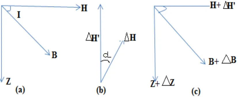
the earth. A magnetic anomaly is now superimposed on the earth’s field causing a change B in
the total field vector B. Let the anomaly produce a vertical component Z and a horizontal
component Hat an angle to H as shown in Figure 3.1(b). Only that part of H which isin the
direction of H, namely H', will contribute to the anomaly (Keary and Brooks, 1984).
H'H cos 3.4
Also,
18
Expansion of the above equation ignoring the negligible terms in yields,
B =Z (Z / B) + H'(H / B) 3.6
Substituting the above equation with angular descriptions of geomagnetic element ratios yields, B Z sin I Hcos
The above approach can be used in calculating the magnetic anomaly caused by a small
magnetic pole of strength m, defined as the effect of this pole on a unit positive pole at the
observation point.
The pole is situated at depth z, a horizontal distance x and radial distance r from the observation point and θ is the angle between a line joining the pole to the observation point to the horizontal.
The force of repulsion Br on the unit positive pole in the direction r is given by,
F =m1 m2/ 4R r
2
Where 1 m and 2 m are magnetic poles of strengths m1and m2separated by a distance r andand
R are constants corresponding to the magnetic permeability of vacuum and relative permeability
of medium separating the poles. The SI unit for is Hm-1 and R is dimensionless (Dentith,
1994).
3.2.1 Geomagnetic field elements
The geomagnetic field, like any magnetic field is a vector field. At any point on the Earth’s
surface it is represented by a vector pointing in the direction of force on a positive pole, and
having a length proportional to the strength of the field at that point. Its components are called
magnetic elements. Among the magnetic elements, the direction of the field is the element least
sensitive to changes in the dimensions and the magnetic properties of the subsurface body. The
19
These elements are represented in the parallelepiped. The angle between the magnetic and the
geographic meridians is the magnetic declination Dwhile that between the total geomagnetic
field vector and the horizontal plane is the magnetic inclination I. These geomagnetic elements vary all over the Earth’s surface. The line where inclination I is zero is the magnetic equator and
points where the inclination is +90 and -90 are the North and South magnetic poles respectively
(Wasilewski, 1973). The total field vector BThas a vertical component BZand a horizontal
component BH in the direction of the magnetic north. The vertical component Z is positive north
of the magnetic equator and negative south of it. The dip of BTis the inclination I of the field.
BTvaries in strength from about 25000nT in equatorial regions to about 70000nT at the magnetic
poles (Parasnis, 1986).
3.2.2 Rock magnetism
All rocks become magnetized because they contain magnetic minerals. Such minerals are
magnetite, hematite, pyrrhotite, ilmenite, maghematite and leucoxenes but magnetite is far the
most common of these minerals. Therefore for most practical purposes, rocks are said to be
magnetic if they contain magnetite and their magnetic properties depend on the amount of
magnetite disseminated among the non-magnetic minerals making up the principal material of
the rock. Magnetite is a representative of the cubic minerals with spontaneous magnetizations
comparable to the familiar ferromagnetic metals (Fe, Co, Ni). Hematite is representative of the
more weakly magnetic, uniaxial minerals, in which the oppositely magnetized sub-lattices of
interacting Fe3+ ions are equally balanced, that is, anti-ferromagnetic but centered at a small
20
The magnetism of a rock may either be induced by the earth’s field or remanent which may have
occurred during cooling or deposition in the rock’s history.
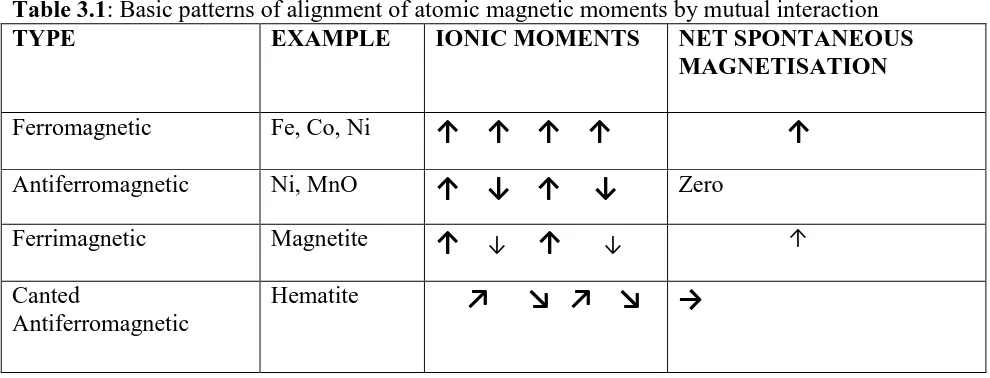
Table 3.1: Basic patterns of alignment of atomic magnetic moments by mutual interaction
TYPE EXAMPLE IONIC MOMENTS NET SPONTANEOUS
MAGNETISATION
Ferromagnetic Fe, Co, Ni
↑ ↑ ↑ ↑
↑
Antiferromagnetic Ni, MnO
↑ ↓ ↑ ↓
ZeroFerrimagnetic Magnetite
↑
↓↑
↓ ↑Canted
Antiferromagnetic
Hematite
↗ ↘ ↗ ↘
→
Induced magnetisation refers to the action of the field on the material where the ambient
field of the earth is enhanced and the material itself acts as a magnet. This magnetisation
is directly proportional to the intensity of the ambient field.
Ii = kF3.9
Where k is the volume magnetic susceptibility, F the ambient field intensity and Iiis the induced
magnetisation per unit volume. The magnetic susceptibility of a rock containing magnetite is
simply related to the amount of magnetite it contains. The remanent magnetization Iris a
permanent magnetisation often predominant in many igneous rocks. This magnetization depends
upon thermal, mechanical and magnetic history of the material and is independent of the field in
which it is measured. The remanent magnetization of a rock may not be in the same direction as the present earth’s field for the field is known to have changed its orientation in geologic time
21 3.3 Ground Magnetic method
Ground magnetic method requires acquisition of measurements of the amplitude of the magnetic
field at discrete points along survey lines, distributed regularly throughout the area of interest
(Telford et al., 1990). The measured magnetic field is the vector sum of; the Earth’s main field,
an induced field caused by magnetic induction in magnetically susceptible earth materials
polarized by the main field, a field caused by remanent magnetism of the earth material and the
other fields less significant caused by solar, atmospheric and cultural influences (Telford et al.,
1976). It is the induced and remanent fields that are of particular interest to geoscientist because
the magnitude of these fields is directly related to the magnetic susceptibility, spatial distribution
and concentration of the local crustal materials.Once the main field and minor sources are
removed from the observed magnetic field data via data reduction and processing methods, the
data are enhanced and presented in readiness for analysis (Milligan and Gunn, 1997). The
analysis ultimatelyleads to an interpretation of structure, lithology, alteration and sedimentary
processes (Mackey et al., 1998).
3.4 Magnetic method in exploration.
In magnetic method we measure the magnetic field produced by the causative source which may be mineral target or the host rock, after correction for the Earth’s magnetic field. Rocks
containing some magnetic minerals are magnetised by induction in the main field and thus
22
This method is suitable in prospection of magnetic minerals or magnetic rocks which are always
host to the target minerals. The method is also used in exploration of geothermal resource by
delineating faults and hydrothermally altered rock. The magnetisation of hydrothermally altered
rocks is normally lower than that of the surrounding rock. Iron ores are usually classified as
strongly and weakly magnetic. Magnetite and hematite deposits of magmatic origin or
hydrothermal replacements type, contact metamorphic deposits and shale, are strongly magnetic
compared to hydrothermal filtration deposits of hematite and siderite and sedimentary deposits
of siderite and limonite which are weakly magnetic. Some manganese and chromium ores are
also highly magnetic and amenable to detection by magnetic method (McEnroe, 1997).
Pyrrholite which is associated with other economic base metal mineralization, ilmenite and other
iron-titanium minerals are indicator minerals. Mineral ores can have magnetic susceptibility
higher or lower than those of the host rock (Dentith, 1994), due to this sharp magnetic contrast,
ground magnetic is selected as a suitable method. For example, at Hired in Iran east, magnetic
susceptibility was measured in one of the target areas and there was good correlation between
gold grade and magnetic susceptibility, 200-3500 x 10-5 SI. Total magnetic field was from
stations and contour maps and models revealed anomalies representing the magnetic responses of
23
CHAPTER FOUR
MATERIALS AND METHODS
4.1 Ground magnetic survey
4.1.1 Introduction
The data acquisition technique involved measurement of the magnetic intensities at discrete
positions along stations regularly distributed within the area of interest so as to cover enough
segment used to determine the structure and the structural history of the study area. Chemical
analysis of soil samples from the area was also undertaken to determine the levels of iron and
titanium oxides. The ground magnetic study of Magaoni, covered an area of about 25 km2, and
consisted of 20 profiles spaced 250m apart. A total of 800 magnetic intensity stations were
measured with spacing of 100m intervals along each line. Each profile had a total length of
4000m and 40 magnetic intensity stations with a bearing normal to the regional structure.
The magnetic intensity measurements were recorded using a Fluxgate magnetometer that gave the earth’s vertical magnetic intensity component. Observations were made along a series of
stations with equal spacing, where the magnetic intensities and station coordinates recorded at a
stationary point. Stations were established using GPS (Global Positioning System) device, to
give their exact positions on the earth in terms of northing and easting coordinates. A special
station known as a Base Station was also established using the same positioning device. Base
24 4.2 Field Equipment
4.2.1 Global Positioning System (GPS)
The Global Positioning System (GPS) is made up of a network of 24 satellites put into orbit by
the U.S Department of Defense. The GPS satellites orbit the earth twice a day and transmit
information to the earth. GPS receivers take this information and use triangulation to calculate the user’s exact location. Essentially, the GPS receiver compares the time a signal was
transmitted by a satellite with the time it was received. The time difference tells the GPS receiver
how far away the satellite is. With distance from a few more satellites, the receiver can determine the user’s position and display it on the instruments electronic map. A GPS receiver must be
locked on to the signal of at least three satellites to calculate a 2D position (latitude and
longitude) and track movement. With four or more satellites in view, the receiver can determine the user’s 3D position (latitude, longitude and altitude). Once the user’s position has been
determined, the GPS unit can calculate other information, such as speed, bearing, track, trip
distance, distance to destination, sunrise and sunset time and more.
4.2.2 Flux Gate Magnetometer
Fluxgate magnetometer uses electromagnetic induction concepts. It consists of two permeable
coils that are wound inopposite directions.The coils are driven with AC signal to saturation. A
secondary coil is wound around both cores to detect changes in magnetic field. In absence of
25
In presence of external magnetic signal, one primary coil will saturate before the other, creating
an imbalance in magnetic field to be detected via EM induction in secondary coil. It has a typical
accuracy of 5 to 10 nT (Force, 1991).
4.3 Field Measurements
Magnetic data measurements were taken at 800 stations, distributed equally on 20 profiles. Three
readings were taken at each station and average calculated to reduce errors. A base station was
carefully established and was preoccupied after every two to three hours. The reading from the
base station was used to correct for diurnal variation. The raw magnetic data are shown in the
appendix.
4.4 Magnetic Data Correction
The reduction of magnetic data was done to remove all causes of magnetic variation or drift from
the observations other than those arising from the magnetic effects of the subsurface geology.
This simply means, processing the data collected to prepare them for interpretation.
4.4.1 Diurnal Variation Correction
This is done to remove the temporal variation of the earth’s main field caused by the action of
solar wind. It is achieved by subtracting the time synchronized signal, recorded at the base
station, from the survey data. The procedure relies on the assumption that the temporal variation
of the main field is the same at the base station and in the survey area. Diurnal variation is small
26
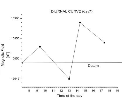
In this study, the base station was preoccupied after every two to three hours and diurnal curve
plotted for the base station data. The diurnal curves were plotted for all the eleven days of the
study and the following general formula was used to do the corrections. The correction was done
on every raw data from every station for each day of the survey, using equation 4.1.
Observed value = raw magnetic value – diurnal variation correction 4.1
.
Figure 4.1 Diurnal curve for day seven (19/08/2014) of the study.
8 9 10 11 12 13 14 15 16 17 18 19 15945 15950 15955 15960 Ma g n e ti c F ie ld (n T )
Time of the day
DIURNAL CURVE (day7)
27 4.4.2 Geomagnetic Correction
It is the removal of the strong influence of the Earth’s main field from the survey data. The most
vigorous method of geomagnetic correction is the use of the IGRF i.e. International Geomagnetic
Reference Field is generally used for this purpose which expresses the undisturbed geomagnetic
field in terms of large number of harmonized and includes temporal terms to correct for secular
variation. This is done because the main field is dominantly influenced by dynamo action in the
core not related to the geology of the upper crust (Lewis, 2000). This is achieved by subtracting a
model of the main field from the survey data. In this survey, the IGRF values were obtained from
an online calculator, based on dates, elevation and geographical location of the station or survey
area. The IGRF values were subtracted from the measured data for all the stations. The anomaly
obtained was used to plot a magnetic contour map and profiles of the survey area using Golden
Surfer8 software.
4.5 Data Enhancement
The magnetic data collected in the study area was processed so as to prepare the dataset for
interpretations. Enhancement simplifies the anomalies, making features of particular interest
more prominent at the expense of others and makes attempt to relate the measured field to the
property being investigated.
4.5.1 Trend Analysis
This is the removal of the influence of magnetic field of deep seated structures (regional) which
28
analysis or regional removal was done to the data of this survey, since the ilmenite being
investigated is a shallow mineral. The following equations were used for trend analysis of the 7 profiles, AA’, BB’, CC’, DD’, EE’, FF’ and GG’ respectively;
Y=0.00334X+650 4.2
Y=0.004X+627.2134 4.3
Y=-0.0181X+656.2134 4.4
Y=0.0364X+540.0974 4.5
Y=.-0.035X+614.1949 4.6
Y=-0.0483X+646.0034 4.7
Y=-0.0035X+618.1346 4.8
X is the station position and Y is the regional field. Regional field is then subtracted from the
corrected that at every X position along a profile. This was done to all the seven profiles.
The following formula was used to obtain the residual. Residual is the magnetic field of the
shallow structures, which were of interest in this survey.
Residual field= corrected data – Regional field.
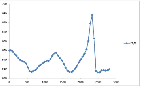
4.9Figure 4.2a shows a shift from zero, along the vertical axis. This is an indication of the presence of regional in the data along profile AA’.Figure 4.2b displays the data along the same
29 Figure 4.2a A graph of profile AA’ with regional
Figure 4.2b. A graph of profile AA’ without regional
620 630 640 650 660 670 680 690 700
0 500 1000 1500 2000 2500 3000
Ряд1
-30 -20 -10 0 10 20 30 40 50
0 500 1000 1500 2000 2500 3000
30 4.5.2 Reduction to the pole
This involves transforming the data to that which would be measured at the earth’s magnetic
poles. This simplifies the anomalies by centring anomalies over the causative magnetic body
rather than being skewed and offset to one side. In this survey, data was reduced to the pole
using Euler software.
4.5.3 Vertical and Horizontal derivatives.
This enhancement quantifies the spatial rate of change of the magnetic field in vertical and
horizontal directions of the profile. Derivatives essentially enhance high frequency anomalies
relative to low frequencies. Euler software was used to do derivatives of the data in this study.
4.5.4 Euler deconvolution
Euler deconvolution is an imaging technique for estimating location and depth to magnetic
anomaly source. It relates the magnetic field and its gradient components to the location of the
anomaly source with the degree of homogeneity expressed as a structural index and it is a
suitable method for delineating anomalies caused by isolated and multiple sources (El Dawi et
al., 2004). Euler deconvolution is expressed in Equation as:
n
B T
x T z z y T y y x T x
x
0 0
0 4.9a
Applying the Euler’s expression to profile or line-oriented data (2D source), x-coordinate is a
measure of the distance along the profile and y-coordinate is set to zero along the entire profile.
Equation 4.6 is then written in form of Equation as:
n
B T
z T z z x T x
x
0
31
Where ( x0, z0)is the position of a 2D magnetic source whose total field T is detected at (x, z) .
The total field has a regional value of B, and n is a measure of fall - off rate of the magnetic field.
n is directly related to the source slope and is referred to as the structural index and depends on
the geometry of the source (El Dawi et al., 2004). Estimating depth to magnetic anomaly using
Euler deconvolution involves: Reduction to the pole, which means transforming the data to that
which would be measured at the magnetic poles of the earth. This simplifies the anomalies by
centering anomalies over the causative magnetic body rather than being skewed and offset to one
side. And calculation of horizontal and vertical gradients of magnetic field data, which quantifies
the spatial rate of change of the magnetic field in vertical and horizontal directions. Derivatives,
essentially enhances high frequency anomalies relative to low frequencies.
4.6 Chemical analysis of samples
Five stations from the study area were selected randomly and soil samples collected from various
depths, ranging from surface to about 50cm depth. The soil samples were collected in transparent
plastic bags and labelled by pens with non-metallic ink to avoid contamination. The samples
were taken to the geology laboratory in to analyse for iron and titanium oxide. Energy Dispersive
X- ray Fluorescence Spectrometry (EDXS), was used for the analysis of the two minerals oxide.
4.6.1 Titanium
It is one of the lightest members of the first row transition series of elements, and belongs to
group four of the periodic table. It is a common lithophile metallic element that forms several
minerals, including ilmenite, rutile, brookite, anatase among others. It exists as titanium dioxide
(TiO2) and has a crustal abundance of 6320 mg kg-1 (Fyfe, 1999). The global average for the soil
32
factor of Ti to TiO2 is 1.668. The median TiO2 is 0.57 % in both subsoil and top soil, with a
range varying from 0.012 to 3.14 % in subsoil and 0.021 to 5.45 % in top soil. These values are
lower in alluvial areas for both top and subsoil (Kabata-Pendias, 2001).
The median TiO2 content in stream sediments is 0.62 % with a range from 0.016 to 4.99 %. High
values in stream sediment (> 0.82 %) are located mainly in areas with outcropping Palaeozoic
and crystalline basement rocks of intermediate to mafic signatures (Mielke, 1979). In floodplain
sediments, the values of TiO2 vary from 0.05 to 2.15 % with a median of 0.48 %. High values are
found in areas with mafic and ultra-mafic crystalline rocks. In floodplain sediment, TiO2 shows
very strong positive correlation with Nb, V, Fe2O3, Co and Al2O3 (Fyfe, 1999).
4.6.2 Iron (III) Oxide
Iron (III) oxide or Ferric oxide is an inorganic compound with formula Fe2O3. It is one of the
main oxides of iron, the other two being Iron (II) oxide (FeO) which is rare and Iron (II,III) oxide
which also occurs naturally as mineral magnetite (Fe3O3). As the mineral known as hematite,
Fe2O3, is the main source of iron for the steel industry. Hematite is weakly magnetic and
normally combine with titanium dioxide to form ilmenite, this explains why ilmenite is weakly
magnetic (Morris, 1980).
4.6.3 Energy Dispersive X – Ray Fluorescence Spectroscopy
Spectroscopy is the study of the interaction between matter and radiated energy. Spectroscopy
data is often represented by a spectrum, a plot of the response of interest as a function of
wavelength or frequency. Spectral measurement devices are spectrometer. Spectroscopy is used
33
result, these spectra can be used to detect, identify and quantify information about the atoms and
molecules. One of the central concepts in spectroscopy is a resonance and its corresponding
resonant frequency. A plot of amplitude against excitation energy will have a peak centred at the
resonance frequency. This plot is one type of spectrum with the peak often referred to as spectral
line and most spectral lines have a similar appearance. In many applications, spectrum is
determined by measuring changes in the intensity or frequency of this energy (Korkish, 1989).
Spectroscopy can be distinguished by nature of the interaction between energy and the material.
It involves absorption and emission of energy by atoms after being irradiated. These absorptions
and emissions are due to electronic transitions of outer shell electrons as they rise and fall from
one electron orbit to another. Atoms also have distinct x-ray spectral that are attributable to the
excitation of inner shell electrons to excited state. Atoms of different elements have distinct
spectra and therefore atomic spectroscopy allows for the identification and quantification of a sample’s elemental composition. In this study, X-ray spectroscopy was used to test for titanium
and iron oxides. The equipment used is known as EDX machine. EDX systems are attachments
to Electron Microscopy instruments or Transmission Electron Microscopy instruments where the
imaging capability of the microscope identifies the specimen of interest (Fyfe, 1999).
The data generated by EDX analysis consist of spectra showing peaks corresponding to the
elements making up the true composition of the sample being analyzed. In this study, Energy
Dispersive X-ray Fluorescence spectrometer was used to analyze for titanium and iron oxides.
34
unique X-rays that are emitted from the samples. Such X-rays are known as “fluorescent X-rays”
and they have unique wavelength and energy that is characteristic of each element that generates
them. Consequently, qualitative analysis can be performed by investigating the wavelength of the
X-ray. As the fluorescent X-ray intensity is a function of the concentration, quantitative analysis
is also done by measuring the amount of X-rays at the wavelength specific to each element
(Fyfe, 1999).
35
RESULTS AND DISCUSSION
5.1 Introduction
Interpretation of magnetic data can be done either qualitatively or quantitatively. In this research
work both methods were applied. The qualitative part is largely visual inspection of magnetic
map. The resultant preliminary structural element map is the cornerstone of the interpretation.
Qualitative interpretation involved recognition of the nature of discrete anomalous bodies
including faults and ventricular intra-sedimentary bodies and deposited features among others.
The most important element in this preliminary qualitative stage was not the interpretation of
anomalous bodies themselves but rather the network of shallow magnetic signatures and discrete
anomalies that at first sight may appear as a pattern of unrevealed anomalies.
In quantitative interpretation, due to the inherent ambiguity in the interpretation of potential field
data, it is not always advisable to go straightforward into solutions interpretation without having
a rough idea about the causative bodies. First of all, the geology of the area was considered,
including a study of all available information on the range of values of the intensity and
inclination of the magnetization of the local rocks, and their distribution. Quantitative
interpretation involves making inferences on the location, depth and shape of the anomaly
causative body. In this study, Euler deconvolution technique was used for quantitative
interpretation.
36
The magnetic intensity colour map shows that there entire study area has weak magnetisation
spread out (Figure 5.1). This indicates that the area is covered by sedimentary deposits of
magnetically weak minerals or materials. The map also shows that the magnetic materials or
minerals covering the area are shallow.
Easting (M)
Metre
Figure 5.1 Magnetic intensity colour map for Magaoni.
No rt hi ng ( M )
37
Contour map just like the intensity colour map, shows that the whole area has weak and shallow
magnetisation. The magnetic signatures are more pronounced in NE, SE, NW and SW of the
area. The magnetisation of the area trends in the N-S direction, as shown in figure 5.2.
Figure 5.2 Magnetic Anomaly contour map for Magaoni.
The 3D anomaly map shows the distribution of magnetic signatures of the area, it gives the
location and quantity of magnetisation in the area, (Figure 5.3). The broad and low amplitude
shown by the colours, represent shallow and weak magnetisation of the area. The three points
where there is sharp and high amplitude of the colours, indicate buried strong magnetic materials
38 Figure 5.3 3D magnetic anomaly map for Magaoni.
Qualitative interpretation of the magnetic field intensity shows higher magnetic values to the
north-east direction running through to the south-west (640nT). The probable cause of this high
magnetic signature could be the due to the presence of iron ores which have high magnetic
susceptibility. This is in agreement with the geologic description of the orientation of ferrous
deposits in Kwale region. The location of ilmenite deposit is characterized by very low and
shallow magnetic anomaly as revealed in the map. The deposits on the northern part of the
region and that on the southern part lie on the relatively low magnetic intensity regions, that is, NORTHING (M)
ANOMALY (nT)
EASTING (M)
39
530nT and 550nT respectively. In the NW and SW orientation are regions of low magnetic
intensities indicating the presence of magnetically weak minerals such as ilmenite deposits with
the same orientation. Thus, low magnetic intensities in the NW and SW orientation as evidenced
in the anomaly map are due to weak magnetic minerals to non-magnetic minerals as a result of
presence of small quantity of iron.
5.3 Interpretation of magnetic data along the profiles
Figure 5.4 shows Euler solutions for magnetic anomaly along profile AA’. Here, three distinct
trends are evident which coincide with the location of ilmenite deposits within the study area.
The profile begins with a relatively low magnetic anomaly points which could be the mineral
sand layer. The next zone (550m-650m) shows no magnetic sources. The lack of magnetic
sources exists mostly between the faults or underground pits. These signatures are followed to
the south by relatively high signatures (600m-1000m and 2000m - 2500m) along the profile and
are postulated to be magnetic mineral. The entire profile is characterized by small amplitude
40
Figure 5.4: Euler depth solution along magnetic anomaly profile AA’
Figure 5.5 shows high magnetic signatures at a depth of about 90m below the surface for profile BB’ at 100m-300m along the profile and these are associated with iron or other magnetic bodies.
Horizontal and vertical gradients highly fluctuate over a distance 800m (0m-800m) along the
profile. This represents abrupt lateral change in magnetization. The sharp and high amplitude of
the anomalies between 400m and 450m, strong and shallow magnetisation which could be
41
Figure 5.5: Euler depth solution along magnetic anomaly profile BB’
In profile CC’ as shown in figure 5.6, there is concentration of Euler solutions between 1600m
and 1800 along the profile an indication of a strong and shallow magnetic source body at a depth
ranging from the surface to about 70m. The profile shows discontinuities between 100m-900m
and 1100m- 1500m, an indication of a fault or underground pits. The largest part of the profile
42
Figure
5.6: Euler depth solution along magnetic anomaly profile CC’
Figure 5.7 shows three distinct anomalies along profile DD’. There exist high magnetic sources
around (0m - 100m), (800m - 1200m) and (1500m-2400m) which is an indication of highly
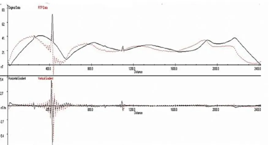
magnetic materials near the surface. The shoulder of the reduction to the pole (RTP) outlines the
edge of a possible magnetic structure located at profile distance.
43
Figure 5.8 shows profile EE’. There is an abrupt change in magnetisation between 900m and
1600m along the profile. This represents the existence of a magnetically strong source lying
between 0m-300m depth, and a very low magnetic signature between 0m – 900m along the
profile which could be an indication of a buried pit zone. The discontinuity shown by the
solution between 300m and 700m could be a fault.
Figure 5.8: Euler depth solution along magnetic anomaly profile EE’
Figure 5.9 shows Euler solution for profile FF’. Horizontal and vertical gradients highly fluctuate
over the entire profile, this indicates change in magnetisation over distance. Sharp and high
amplitudes of the anomalies at 1000m and 1500m along the profile, clearly indicate shallow
magnetic structures. Cluster is observed along the entire profile, this shows the presence of
44
Figure 5.9: Euler depth solution along magnetic anomaly profile FF’
It is evident in figure 5.10 that Euler solution for profile GG’ shows magnetisation at a depth of
about 450m from 0m to 500m along the profile. Between 500m and 1000m, there is a
discontinuity which could possibly be a buried it or fault. There is clustering between 1000m and
2500m, indicating presence of shallow magnetic bodies around that region. There is an abrupt
change in both horizontal and vertical gradient between 2250m and 2750m, this shows there
45
Figure 5.10: Euler depth solution along magnetic anomaly profile GG’
These undulating signatures and the Euler deconvolution solutions clearly show shallower
subsurface magnetic deposits within the geological area.
5.4 Interpretation of the chemical analysis result.
Sample SS13 was obtained from the surface at station N9516376, E0551360, SS16 was obtained
from a depth of 0.5m at N9519776, E0551610, SS20 from a depth of about 1m at N9518276,
E0553610, SS21 was taken from the surface at N9516476, E0555860 and sample SS24 was
taken from a depth of about 0.7m at N9520176, E0555110. Table 5.1 shows the quantitative
analysis results from EDX Fluorescence Spectroscopy of the soil sample SS13. The result gives
the highest percentage for silicate (SiO2 92 %), this was expected because the area is full sand
46
was found to be 4.4 %, this is way above the global average of TiO2 in the soil which is
approximately 0.7 %. Iron III Oxide (Fe2O3) was in small quantity, about 1.7 %. Considering the
percentage oxides of iron and titanium, it shows the likelihood of the existence of leucoxene,
which is altered ilmenite arising due to the leaching of iron.
Results for sample SS16 shows greatest percentage of silicate due to the abundance of sand in
the area ( SiO2 79.9 %), as shown in table 5.2. From the same sample, we see an elevated value
of titanium dioxide (TiO2 13 %), it is so much above the average value for sedimentary deposit.
Comparing the percentage of titanium dioxide and that of Fe2O3 which is approximately 4 %, it
clearly indicates the presence of ilmenite or leucoxene. Table 5.3 shows analysis result for SS20
showing high values for SiO2 82.87 % and Al2O3 10.24 %, this may represent the availability of
bauxite in the area. The percentage values for titanium dioxide which was 2.898 % and that of
iron (iii) oxide about 2.151 % shows the presence of heavy minerals could be ilmenite since the
difference in the percentage oxide for iron and titanium is not that much.
Sample SS21 also had a high value of silicate (SiO2 90.955 %), evident in table 5.4, showing
abundance of sand in the study of area. There is an elevated value for titanium dioxide (TiO2
4.575 %) and a lower value for iron oxide (Fe2O3 1.554 %), this is evident that ilmenite or
ilmenite in form of leucoxene exists in the sample. The result for SS24 shows high values for
silicate and bauxite. Iron and titanium oxides have 3.678 % and 3.178 % respectively, as shown
in table 5.5, these values correlate well with the existence of ilmenite. All the three samples gave
47
comparing with the values for iron oxide, they indicate the presence of ilmenite and leucoxene.
The samples also showed presence of zircon which is a heavy mineral sand and normally occurs
with rutile and ilmenite.
48 Table 5.2 Analysis result for sample SS16
49
Table 5.4 Analysis result for sample SS21