LI, JIANGTIAN. Towards Transparent Parallel Processing on Multi-core Computers. (Under the direction of Professor Xiaosong Ma).
Parallelization of all application types is critical with the trend towards an expo-nentially increasing number of cores per chip, which needs to be done at multiple levels to address the unique challenges and exploit the new opportunities brought by new architecture advances. In this dissertation, we focus on enhancing the utilization of future-generation, many-core personal computers for high performance and energy effective computing.
On one hand, computation- and/or data-intensive tasks such as scientific data processing and visualization, which are typically performed sequentially on personal work-stations, need to be parallelized to take advantage of the increasing hardware parallelism. Explicit parallel programming, however, is labor-intensive and requires sophisticated per-formance tuning for individual platforms and operating systems. In this PhD study, we made a first step toward transparent parallelization for data processing codes, by devel-oping automatic parallelization tools for scripting languages. More specifically, we present pR, a framework that transparently parallelizes the R language for high-performance sta-tistical computing. We apply parallelizing compiler technology to runtime, whole-program dependence analysis and employ incremental code analysis assisted with evaluation results. Experimental results demonstrate that pR can exploit both task and data parallelism trans-parently and overall achieve good performance as well as scalability. Further, we attack the performance tuning problem for transparent parallel execution, by proposing and designing a novel online task decomposition and scheduling approach for transparent parallel com-puting. This approach collects runtime task cost information transparently and performs online static scheduling, utilizing cost estimates generated by ANN-based runtime perfor-mance prediction, as well as by loop iteration test runs. We implement the above techniques in the pR framework and our proposed approach is demonstrated to significantly improve task partitioning and scheduling over a variety of benchmarks.
by Jiangtian Li
A dissertation submitted to the Graduate Faculty of North Carolina State University
in partial fulfillment of the requirements for the Degree of
Doctor of Philosophy
Computer Science
Raleigh, North Carolina 2008
APPROVED BY:
Dr. Frank Mueller Dr. Nagiza Samatova
Dr. Xiaosong Ma Dr. Xiaohui Gu
DEDICATION
To my parentsGuangyi Li, Jianfen Huang
and
BIOGRAPHY
ACKNOWLEDGMENTS
This dissertation would not have been accomplished without the support and in-spiration of many people.
First of all, I would like to express my deep gratitude to my advisor, Dr. Xiaosong Ma, for her expert guidance, consistent support, and patience to shepherd me in my Ph.D. pursuit. I feel very fortunate to have such a great mentor leading me through my research with insightful thoughts and sound advice. I am also much indebted to Dr. Nagiza Samatova for mentoring me and initializing the pR project, particularly during my internship and visits at Oak Ridge National Laboratory. Her knowledge and suggestions have been of great value to me. Also I would like to convey my appreciation to Dr. Xiaohui Gu and Dr. Frank Mueller for serving on my advisory committee and offering me valuable suggestions on my dissertation.
I am grateful to the ORNL team in the development of the pR prototype: Srikanth Yoginath and Guruprasad Kora for important contributions in code, thoughts, and discus-sions. Besides, they provided great convenience during my stay at Oak Ridge. Also I am grateful to our collaborators at LLNL and Cornell University: Karan Singh, Dr. Martin Schulz, Dr. Bronis de Supinski, and Dr. Sally McKee for valuable suggestions, software support and assistance in paper writing.
I want to thank all the members in PALM group for their friendship and the fun time spent together in the lab. Thanks to Heshan Lin for his generous help since I came to NCSU. I benefit a lot from brainstorming research ideas and discussing technical problems with him. Thanks to Zhe Zhang, Tao Yang, and Feng Ji for their unselfish help in research, courses, and in life.
My sincere thanks also go to Mihye Ahn, Tyler Bletsch, Kristy Boyer, Jaydeep Marathe, Ripal Nathuji, Christopher Symons, Vivek Thakkar, Chao Wang for their warm-hearted help during my doctoral research.
TABLE OF CONTENTS
LIST OF TABLES . . . viii
LIST OF FIGURES . . . ix
1 Introduction . . . 1
1.1 Problem Statement and Motivation . . . 1
1.2 Contributions . . . 3
1.3 Dissertation Outline . . . 5
2 Transparent Parallelization of the R Scripting Language . . . 6
2.1 Motivation for Transparent Parallel Data Processing . . . 6
2.2 Background information of R . . . 8
2.3 pR Architecture . . . 9
2.3.1 Design Rationale . . . 9
2.3.2 Framework Architecture . . . 10
2.4 pR Design and Implementation . . . 12
2.4.1 The Analyzer . . . 12
2.4.2 The Parallel Execution Engine . . . 17
2.5 Ease of Use Demonstration . . . 18
2.6 Performance Evaluation . . . 20
2.6.1 Synthetic Loop . . . 20
2.6.2 Boost . . . 21
2.6.3 Sensor Network Code . . . 22
2.6.4 Bootstrap . . . 23
2.6.5 SVD . . . 24
2.6.6 Overhead Analysis . . . 24
2.6.7 Task Parallelism Test . . . 27
2.7 Summary . . . 28
3 Autonomic Task Scheduling . . . 30
3.1 Motivation . . . 30
3.2 Background on Artificial Neural Networks . . . 33
3.3 ASpR System Architecture . . . 34
3.4 Function Performance Profiling and Model Construction . . . 36
3.5 Loop Cost Prediction through Test Driving . . . 37
3.6 Task Partitioning and Scheduling . . . 38
3.7 Experimental Results . . . 42
3.7.1 Sample Schedule . . . 42
3.7.3 Benchmark Generation . . . 45
3.7.4 Accuracy and Overhead of Online Prediction . . . 47
3.7.5 Impact on Transparently Parallelized R Code Execution . . . 49
3.7.6 Real-world Application Performance Results . . . 53
3.8 Summary . . . 54
4 Energy and Performance Impact Analysis . . . 56
4.1 Motivation . . . 57
4.2 Workloads . . . 58
4.2.1 Native Workloads . . . 58
4.2.2 Foreign Workloads . . . 61
4.3 Methodology . . . 62
4.3.1 Objectives and Metrics . . . 62
4.3.2 Experimental Platform . . . 63
4.3.3 Measurement Scheme . . . 64
4.4 Results . . . 66
4.4.1 Impact of Concurrency in the Cluster Mode . . . 66
4.4.2 Consolidated Execution in Native OS . . . 67
4.4.3 Consolidated Execution with Virtual Machine . . . 71
4.4.4 Throttling with Vulnerable Workload . . . 72
4.5 Summary . . . 73
5 Related Work . . . 80
5.1 Transparent Parallelization . . . 80
5.2 Performance Prediction and Self-learning Systems . . . 83
5.3 Resource Allocation and Task Scheduling . . . 84
5.4 Energy-aware Computing . . . 85
5.5 Co-scheduling and Performance Impact . . . 87
6 Conclusions and Future Work . . . 88
LIST OF TABLES
Table 2.1 Itemized overhead with the Boost code, in percentage of the total execution
time. The sequential execution time of Boost is 2070.7 seconds. . . 25
Table 2.2 Itemized overhead with the sensor network code, in percentage of the total execution time. The sequential execution time is 825.2 seconds. . . 25
Table 2.3 Itemized overhead with the bootstrap code, in percentage of the total execution time. The sequential execution time of bootstrap is 2918.2 seconds. . . 25
Table 2.4 Itemized overhead with the SVD code, in percentage of the total execution time. The sequential execution time of SVD is 227.1 seconds.. . . 26
Table 2.5 The parallel execution time and speedup of the task parallelism test script . . 28
Table 3.1 MCP overhead in seconds measured in our testbed . . . 44
Table 3.2 Description of selected R functions and their arguments in the experiments. Aand B denoten×nnumeric matrices. . . 45
Table 3.3 Overview of parameter spaces of selected R functions used in the experiments. NAand NB denote their sizes in terms of the number of double-precision numbers. 46 Table 3.4 Performance summary of ASpR on the 100 automatically generated microbench-marks. . . 49
Table 3.5 ASpR and dependent microbenchmarks (8 procs) . . . 51
Table 3.6 Overview of tasks in the real R application. . . 53
Table 4.1 Benchmarks used as native workloads . . . 59
Table 4.2 Benchmarks used as foreign workloads . . . 59
Table 4.3 L2 cache miss ratios of native workloads . . . 70
Table 4.4 Average CPU utilization and power consumption of native workloads, running alone or with foreign workloads . . . 70
LIST OF FIGURES
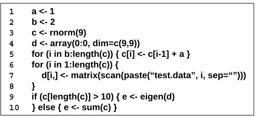
Figure 2.1 A sample R script . . . 9
Figure 2.2 pR Architecture . . . 11
Figure 2.3 The pR analyzer’s internal structure . . . 12
Figure 2.4 A sample parse tree and a sample task precedence graph. In the task prece-dence graph, the depenprece-dence analysis first pauses at task 4 since the loop bound is unknown at that point. The analysis resumes when task 2 completes and the loop bound is evaluated. A similar process repeats for all the other pause points. . . 13
Figure 2.5 Comparison with the snow package interface . . . 19
Figure 2.6 Performance of pR with various benchmarks. Error bars are omitted since variances are small. The average 95% confidence interval (CI) of pR is 0.98% and maximum 95% CI is 2.86%. (a) Performance with the synthetic loop code. (b) Performance with the Boost application. . . 20
Figure 2.7 Performance of pR with various benchmarks. Error bars are omitted since variances are small. The average 95% confidence interval (CI) of pR is 0.98% and maximum 95% CI is 2.86%. The average 95% CI of snow is 1.44% and maximum 95% CI is 5.63%. (a) Performance with the sensor network code. (b) Performance with the bootstrap code. (c) Performance with the SVD code. . . 22
Figure 2.8 The task parallelism test code . . . 27
Figure 3.1 A sample R script . . . 31
Figure 3.2 A motivating example with sample schedules that show task lengths propor-tional to their execution time on an eight core system . . . 31
Figure 3.3 A sample feed-forward neural network . . . 33
Figure 3.4 A sample hidden layer unit with a sigmoid activation function (borrowed from [81]) . . . 34
Figure 3.5 Adaptively Scheduled parallel R (ASpR) architecture overview . . . 35
Figure 3.7 Comparison with dynamic scheduling . . . 43
Figure 3.8 Online training accuracy and overhead for various training data sizes . . . 48
Figure 3.9 Average normalized improvement for “top 10” microbenchmarks . . . 50
Figure 3.10 Comparison of scheduling approaches on “top 10” microbenchmarks . . . 52
Figure 3.11 Comparison of scheduling approaches on the real R application . . . 54
Figure 4.1 Power states of Thinkpad t61 . . . 58
Figure 4.2 Power Experimental Setup . . . 63
Figure 4.3 Measurement scheme overview . . . 65
Figure 4.4 Performance/energy efficiency of foreign workloads on 8-core server with var-ied level of concurrency . . . 67
Figure 4.5 Energy saving of consolidated execution in the native OS. The pair of numbers above each group of bars showESRC/ESRV for that workload combination. . . 75
Figure 4.6 Performance impact when workloads consolidated in the native OS . . . 76
Figure 4.7 Energy saving of consolidated execution in VM. The pair of numbers above each group of bars showESRC /ESRV for that workload combination. . . 77
Figure 4.8 Performance impact with foreign workloads running in VM . . . 78
Chapter 1
Introduction
1.1
Problem Statement and Motivation
General-purpose computing is taking an irreversible step toward parallel architec-tures, as stated in a recent report on the landscape of parallel computing research [4] by researchers from Berkeley. The number of cores on a chip is expected to double with each semiconductor process generation. As we enter this multi-core era, we are facing unprece-dented challenges and opportunities for scientific computing and data analytics.
On one hand, multi-core computers will greatly benefit scientific data analytics in particular, as it is traditionally performed in personal computing settings. The increasing number of cores provides more computing power and degree of parallelism at the thread level. This brings good news to scientific data analytics, which is a complex but inherently parallel process. It is often highly repetitive: performing the same set of statistical functions iteratively over many data objects, which are generated from different time-steps, data partitions, etc.
Moreover, the single-computer parallel data processing can naturally be extended to use multi-computer environments, through mechanisms such as volunteer computing, as a result of relatively loosely coupled relationship between work units. In this regard, projects such as BOINC [19] and CONDOR [73] have been deployed for parallel execution of data processing tasks [31, 37, 63, 89, 115]. The high-impact BOINC project consists of independent work units and is naturally parallel.
tools or libraries that could efficiently exploit this parallelism. Unlike simulations that have utilized supercomputers for decades, which commonly use general-purpose, compiled languages (such as C, C++, and Fortran), as well as well-adopted parallel interfaces (such as MPI and OpenMP), data processing programs are often written in scripting languages and are currently much less likely parallelized. Further, parallel computing techniques used predominantly on clusters often are not applicable or usable for parallel data analysis.
In particular, several concerns arise with respect to the ease-of-use and energy-efficiency of parallel data analytics, which potentially hurdle the effective utilization of the underlying architecture parallelism.
First, the complexity of parallel programming is well known and has been doc-umented in the literature [78, 91]. One widely adopted parallel programming model is message passing [49]. However, this model requires that programmers have parallel pro-gramming skills to specify ways of data partitioning, task scheduling and inter-process syn-chronization, which are challenging, time-consuming, and platform-dependent tasks. Most data processing tool developers are domain scientists, who prefer spending time studying their data than developing parallel codes and dealing with the porting/execution overheads associated with explicit parallel programming. One alternative to explicitly parallel pro-gramming is to let the compiler perform parallelization work and produce binaries that can be executed in parallel [1, 5, 7, 18, 54]. The research has been conducted for programming languages such as C and Fortran. However, to the best of our knowledge, little work has been done in automatic parallelization for interpreted languages, which are used in popular data processing tools such as Matlab [77] and R [96].
Even with compiler technology transplanted to the scripting language problem, transparent parallel data processing tools must be able to exploit bothtask parallelismand
identify both kinds of parallelism and coordinate resources wisely to achieve a better overall performance.
Finally, while performance may remain the dominating goal for scientific comput-ing and data analytics, the energy cost has become an increascomput-ing concern. High-end server systems and clusters have traditionally been used to deliver higher performance in scientific computing. However it comes at the energy cost of operating and cooling of server systems. With more powerful multi-core personal computers, offloading scientific workloads to per-sonal computers and utilizing their idle cores provides an alternative that can potentially save energy. On the other hand, though the multi-core architecture naturally provides more room for the concurrent execution of multiple workloads, contention for resources, especially non-CPU ones, can still lead to performance degradation visible to resource owners. How to achieve energy-performance balance for volunteer scientific computing emerges as an urgent question to be answered.
1.2
Contributions
In this dissertation study, we have taken several initial steps towards transparent parallel processing on multi-core computers. Specifically, we addressed the problems out-lined above by examining the ease-of-use and energy-effective side of parallel data processing on multi-core computers.
Regarding user-friendly parallel scientific data processing,we explored transparent parallelization and task scheduling for scripting languages. Major contributions along this direction include:
• We propose a fully transparent self-adaptive, platform- and application-independent loop and task scheduling mechanism, in an effort to optimize pR. We build lightweight online profiling and performance prediction models based on machine learning. More-over, we extend the current static scheduling algorithm to use cost estimates from our models for loop partitioning and task scheduling, and runtime heuristics for more effective processor allocation and scheduling. Our results using both real-world ap-plications and synthetic benchmarks show that our proposed approach significantly improves task partitioning and scheduling, with a maximum improvements of 40.3% and average improvement of 12.3%.
• To our best knowledge, pR is the first transparent parallelizing tool for a scripting language without using special hardware or virtual machine support. Also, we are the first to apply machine learning technology such as Artificial Neural Networks (ANN) to parallel task scheduling. Meanwhile, though our work used R for a proof-of-concept investigation and case study, the techniques developed in this study can be applied in more general settings, such as the transparently parallel execution of other scripting languages, and performance profiling based self-learning systems.
With tools like pR emerging for the next-generation multicore computers, it is more appealing than ever to leverage mechanisms such as volunteer computing, to exploit under-utilized personal computers for high-throughput, computation- and/or data-intensive data processing. To this end, we examined a new computing model, aggressive volunteer computing, which distributes resource-intensive background workloads to active PCs rather than waiting for them to quiet down as done in traditionally volunteer computing.
1.3
Dissertation Outline
Chapter 2
Transparent Parallelization of the
R Scripting Language
In this chapter, we present our first step toward transparent parallel processing on multi-core computers. Given the pressing need for transparent parallelization in scientific data processing nowadays, as we will discuss in details in section 2.1, we tackle the problem by experimenting on the R scripting language, a widely used data processing tool in statisti-cal computing. Section 2.3 and 2.4 present our transparent parallelization framework for R and design and implementation issues, followed by ease-of-use demonstration in section 2.5 and performance evaluation in section 2.6.
The pR framework builds the groundwork of our endeavor in transparent par-allelization for scientific data analytics. It includes fundamental functionalities to handle dependence analysis, task and data distribution, synchronization, and orchestration. Based on this framework, we will further explore possible optimizations in the next Chapter.
2.1
Motivation for Transparent Parallel Data Processing
Ultra-scale simulations and high-throughput experiments have become increas-ingly data-intensive, routinely producing terabytes or even petabytes of data. While most research efforts in scientific computing focused on the data producer side, the growing needs for high-performance data analytics have not been addressed sufficiently.
there have been a number of projects working on parallel tools/libraries for popular scripting languages used by scientists, such as Matlab [77] and R [96] (Section 5.1 gives the detailed description of related work). However, the majority of long-running data processing scripts today remain unparallelized.
Through our interaction with domain scientists, we identified two major fac-tors contributing to the scientists’ reluctance in using existing parallel scripting language tools/libraries. First, there lacks support for transparent parallelization that would enable domain scientists to reuse their existing sequential data analysis codes with little or no changes. Throughout their scientific careers, many scientists have accumulated hundreds or even thousands of lines of their favorite codes. Re-writing or making changes to such collectively lengthy codes is an error-prone, tedious, and painful exercise that scientists will often resist to. Hence, for domain scientists, an approach that does not require explicit parallel programming is highly desirable.
Second, there is not sufficient support to exploit parallelism at multiple levels by an individual tool/library. In most data processing scripts, both task parallelism and
data parallelism are present. For example, computing the eigenvalue decomposition and generating a histogram of a matrix, two common tasks, can be perfectly overlapped and executed in a task parallel fashion. Likewise, a loop processing simulation output files generated in a series of timesteps or a loop processing the elements of a large array may be broken into blocks and executed in a data parallel manner. Currently, existing tools/libraries each only focuses on exploiting one type of parallelism.
In an attempt to approach the above problems, we describe an automatic and transparent runtime parallelization framework for scripting languages. We argue that data dependence analysis techniques developed for compiled languages are more than adequate in parallelizing loops and function calls in data processing scripts. Meanwhile, the interpreted nature of scripting languages provides a very favorable environment for runtime, aggressive dependence analysis that often cannot be afforded by compilers. By using runtime, full-program dependence analysis, our proposed framework does not require any source code modification, and exploits both task parallelism and data parallelism.
back-ground information about R is given in the next section.
2.2
Background information of R
R [96] is an open-source software and language for statistical computing and graph-ics, which is widely used by the statistgraph-ics, bioinformatgraph-ics, engineering, and finance commu-nities. It has a center part developed by its core development team and provides add-on hooks for external developers to add extension packages. The R source codes were written mainly in C. R can be used on various platforms such as Linux, Macintosh and Win-dows and can be downloaded from the CRAN (Comprehensive R Archive Network) site at http://www.r-project.org/.
As a data processing tool, R can perform diverse statistical analysis tasks such as linear regression, classical statistical tests, time-series analysis, and clustering. It also provides a variety of graphical functions such as histograms, pie charts and 3D surface plots. Built upon R, many other data processing software tools are developed, such as BioConductor [14], an open-source, open-development software package for the analysis of biological data.
R is an interpreted language, whose basic data structure is an object. Internally an R object is implemented as a C structSEXPREC, whose naming roughly corresponds to a Lisp “S-expression.” For example, an object may be a vector of numeric values or a vector of character strings. R also provides a list, an object consisting of a collection of objects.
R can be used in both interactive and batch modes. In the interactive mode, R works via a command-line interface. The user retrieves the results from the standard output by typing variable names. In the batch mode, an R script is supplied as a file and is executed from the R prompt. Results can be written into output files or retrieved from the standard output as in the interactive mode. In our research we focus on parallelization of the batch-mode execution.
1 a <- 1
2 b <- 2 3 c <- rnorm(9)
4 d <- array(0:0, dim=c(9,9))
5 for (i in b:length(c)) { c[i] <- c[i-1] + a } 6 for (i in 1:length(c)) {
7 d[i,] <- matrix(scan(paste(“test.data”, i, sep=“”)))
8 }
9 if (c[length(c)] > 10) { e <- eigen(d) 10 } else { e <- sum(c) }
Figure 2.1: A sample R script
Lines 9-10 are a conditional branch. The first branch computes eigenvalues and eigenvectors of the rectangular matrix and the second one finds the summation of all the vector elements.
2.3
pR Architecture
2.3.1 Design Rationale
The approach we adopt in building pR is based on several motivating observations regarding computation-intensive and/or data-intensive R codes:
• As a high-level scripting language, the use pattern of R is significantly different from those of general-purpose compiled languages such as C/C++ or Fortran. Most R codes are composed of high-level pre-built functions [29] typically written in a com-piled language but made available to R environment through dynamically loadable libraries. For example, the R function svd() utilizes LAPACK’s Fortran dgesdd()
code underneath rather than providing an explicit low-level matrix decomposition in a scripting language.
• Several characteristics of the R language simplify dependence analysis. There are no explicit data pointers.1
The input parameters to the functions are read-only, while the modified or newly-created variables by the function are returned explicitly. Returning several such variables is accomplished through the formation of a list object, which is a collection of other objects. This removes the aliasing problem, a major limiting factor in general-purpose compilers. Still, users may call external functions that are written in other languages such as C, which may contain the use of pointers.
As a result, in designing this proof-of-concept parallel R framework, we focus on parallelizing two types of operations: function calls and loops. In a typical computation-intensive R program (and programs in other languages as well), these two form the bulk of the execution time.
The key innovation in the pR design is coupling existing compiler technology with runtime analysis for scripting languages. We perform dynamic dependence analysis before interpreting R statements and identify tasks and loops that can be parallelized. This allows us to go beyond loop parallelization, which has been the primary focus of parallelizing compilers, to also exploit task parallelism between any two statements. Particularly, with run time file information check we can parallelize I/O operations, at least with a file-level granularity. In addition, more aggressive and complete parallelization is achieved through
incremental analysis that delays the processing of conditional branches and dynamic loop bounds until the related variables are evaluated.
2.3.2 Framework Architecture
The key feature of pR is that it dynamically and transparently analyzes a sequential R source script and accordingly parallelizes its execution. The results of partial execution are collected to perform further analysis at run time. The pR framework is built on top of and does not require any modifications to the native R environment. The only external package needed by pR is the standard MPI library [49], for inter-processor communication. When users run their R scripts in parallel using pR, one of the processors, the one with the MPI rank 0, is assigned as the master node, while the others becomeworker nodes. The basic execution unit in pR is an R task (ortaskfor brevity), which is the finest
Analyzer
Parallel Execution
Engine
Local R Process
Frontend
R process Frontend
R process
…
Worker 1 Worker n
Master R script
Figure 2.2: pR Architecture
unit for scheduling. A task is essentially one or multiple R statements grouped together as a result of parsing, dependence analysis and loop transformation. A task can be a part of a parallelized loop, a function call, or a block of other statements between these two types of objects. As shown in Figure3.5, there is an R process running on the master and each of the worker nodes. This process executes R tasks: functions and parallelized loops on the workers and all the other tasks on the master.
The major complexity of pR resides at the master side, which performs dynamic code analysis, on-the-fly parallelization, task scheduling, and worker coordination. These are carried out by two components: an analyzerand a parallel execution engine. The analyzer forms the front-end of our pR system. Its primary functionality is to perform syntactic and semantic analysis of R scripts. Such analysis helps to help pR identify execution units and their precedence relationship. The parallel execution engine works as the back-end of pR and takes input from the analyzer. It is responsible for dispatching tasks, coordinating the communication among the workers, supervising the local R processing, and collecting results.
The analyzer pauses where static analysis is not sufficient to perform paralleliza-tion, such as conditional branches and loops with dynamic bounds. The analyzer resumes its analysis after the parallel execution engine provides appropriate runtime evaluation results. In this case, these results are fed-back to the analyzer, as shown in Figure3.5.
master and other worker nodes. This way, data communication can be performed without interrupting the R task execution carried out by the R process. The front-end process manages the data, tasks, and messages for the worker. It supplies the R process with task scripts and input data, and collects the output data from the latter. The inter-process communication on each node is performed via the UNIX domain sockets.
2.4
pR Design and Implementation
2.4.1 The Analyzer
Parser Dependence
Analyzer
Loop Parallelizer
R Script Parsing Tree Task Precedence Graph
Figure 2.3: The pR analyzer’s internal structure
As illustrated in Figure 2.3, there are three basic modules inside the analyzer: a
parser, adependence analyzer, and aloop parallelizer. Below we discuss the task performed by each of these modules.
Parsing R code The pR parser focuses on identifying R tasks for subsequent execution. Given an input R script, the parser carries out a pre-processing pass of the code using R’s internal lexical functions to identify tokens and statements. The parser then breaks down the script into a hierarchical structure and outputs a parse tree.
The parse tree generated by the pR parser is a simplified version compared to those by compilers. Here the sole purpose of parsing is to perform dependence analysis and automatic parallelization, while the actual interpretation and evaluation of R statements are carried out by the native R environment. Because the basic unit of pR’s task scheduling is at least one R statement, its parse tree stops at this granularity, with each leaf node representing one individual R statement. For all the leaf nodes, the input and output variable names as well as array subscripts, if any, are extracted and stored.
that share the same entry or exit point. A region is a loop (including nested loops), or a conditional branch, or one or more consecutive other statements. For example, a region that goes from the very beginning of a script till the beginning of the first loop or branch within the same scope forms an internal node in the parse tree. A loop makes up another internal node and inside the loop scope, the same procedure of constructing internal nodes recursively applies. Similarly, a conditional branch node includes the if clause and the
else clause (if there is one) and inside the branch scope for which the parsing sub-tree is recursively built in the same way.
Script
Block Loop Loop Branch
Stmt Stmt Stmt Stmt Block Block
Stmt Stmt
IF Block
ELSE Block
Stmt Stmt
(a) A sample parse tree.
ll
a <- 1 b <- 2 c <- rnorm(9) d <- array(0:0, dim=c(9,9))
for (i in b:length(c)) {
c[i] <- c[i-1] + a }
for (i in 1:length(c)) {
d[i,] <- matrix(scan(paste(“ test.data” , i, sep=“ ” ))) }
if (c[length(c)] > 10) {
e <- eigen(d) }
else {
e <- sum(c) }
task 1 task 2 task 3
task 4 task 5
task 6
Pause point
ll
ll
ll
(b) A sample task precedence graph.
Figure 2.4: A sample parse tree and a sample task precedence graph. In the task precedence graph, the dependence analysis first pauses at task 4 since the loop bound is unknown at that point. The analysis resumes when task 2 completes and the loop bound is evaluated. A similar process repeats for all the other pause points.
2.1. The leaf nodes are all statements corresponding to lines 1-4, 7, 11, 15, and 19, respec-tively. Each internal node covers a loop, a branch, or another region in the code, where a “block” stands for a code block that does not contain loops or branches.
Runtime incremental dependence analysis The pR dependence analyzer takes the
parse tree generated by the parser and performs both statement dependence analysis and loop dependence analysis. Because the basic scheduling unit is a task, the dependence analyzer will first group consecutive simple statements (those not containing any function calls) inside non-loop code blocks into tasks. For example, the first two statements in our sample code will become one schedulable R task, which will be executed locally on the master.
In statement dependence analysis, we compare the input and output variables be-tween the statements to identify all three dependence types: true dependence (write-read), anti-dependence (read-write), and output dependence (write-write). Statements depen-dence analysis is applied across the tasks.
One unique contribution of pR is file operation parallelization, where we take a more aggressive approach than compilers do. Traditionally, compilers do not attempt to parallelize operations involving system calls. In the R context, however, users would greatly benefit from parallelizing the analysis of different files (such as a batch of time-series simulation results). This type of processing is very common and the operations across different files are typically independent. Therefore, we perform a runtime file check when determining whether there exists dependence between tasks containing file I/O operations. To handle the aliasing problem caused by file links, we recursively follow symbolic links using the readlinksystem call until a regular file or hard link is reached. The inodes of such files are checked to determine the dependence between I/O operations. In the current prototype the file dependence check is coarse-grain and conservative. Any two operations working on the same physical file are considered dependent. Further, all calls of user-defined functions, each considered as one single task, are considered dependent with any task that performs I/O.
re-quire variable declaration. Meanwhile, the usage of “superassignment” does not necessarily indicate an access to global variables. Therefore a global variable can not be identified in a single step. Fortunately, R uses lexical scoping and global variables can be identified with static whole-program analysis. This allows pR to fix the problem by parsing user-defined function bodies although the current pR prototype does not parallelize these functions. The pR analyzer traverses each parse tree to identify global variables. If a function accesses global variables, we treat them also as input/output parameters of that function call.
Another issue arises when reference objects such as environment are used, since they work as implicit pointers. As a solution, we treat any statement involving reference objects as a barrier to ensure correctness.
Finally, we identified several types of pR operations that require special handling by the analyzer. These operations are “location-sensitive” in the sense that distributing tasks to different nodes, even when they appear to be independent or when they are de-pendent but executed in the correct order, will cause a problem. For example, two function calls both using random number generation (such asrnormshown in our sample code) may yield undesirable results if parallelized. Similarly, file accesses may be a problem. Our coarse-granularity file operation dependence analysis considers two subsequent operations dependent if they access the same file. However, these operations, may yield incorrect re-sults if executed distributedly (albeit sequentially) on two workers, depending on the file system implementation. Accessing the reference objects mentioned above is another exam-ple. Since pR strives to provide transparent parallelization, our current prototype takes the cautious approach by “binding” such location-sensitive operations to one processor. This is done by the analyzer marking certain edges or adding marked edges if necessary in the TPG to instruct the pR scheduler to ensure each group of such dependent tasks be executed on the same processor.
As mentioned in Section 2.3, typical R scripts used in scientific data analysis are not expected to contain elaborate user-defined loops with a complex array index structure. Therefore many mature loop dependence analysis algorithms suffice for pR’s purposes. In our current prototype, we adopted the gcd test [8], a method of data-dependence test generally used in automatic program parallelization. The test compares subscripts of two array variables which are linear (affine) in terms of the loop index variables. Basically, it builds a linear Diophantine equation and calculates the greatest common divisor to see whether a solution to that equation exists. The test is effective for simple array subscripts but gets inefficient for complex array subscripts. Our experience up to now with a limited set of time-consuming R applications show thatgcd test is powerful enough for user-defined loops in R. Plus, pR adopts widely-used compiler data structures and it is easy to plug in different analysis algorithms, in case future pR users encounter applications that call for more sophisticated analysis.
pR takes advantage of the fact that the analysis tool can closely interact with the runtime R interpretation environment to perform incremental analysis. This allows the analyzer to temporarily pause at points where it requires runtime information to continue with the code analysis and parallelization. In this initial implementation, we define an
pause point in the dependence analysis as a task that is either a loop with an unknown outermost loop bound or a conditional branch that contains function calls or loops. These tasks are considered worth parallelization and remote execution, but cannot be parallelized (or parallelized aggressively enough) before runtime. When the key evaluation results are returned from the execution engine, the analysis and parallelization resumes and advances to the next pause point or the end of the script.
The precedence relationship among the tasks is stored in a task precedence graph (TPG), as the output of the dependence analyzer. A TPG is essentially a directed acyclic graph, where each vertex represents one task and each directed edge represents the depen-dence between two tasks. In addition, if the task consists of a loop, the dependepen-dence distance (defined as the difference between dependent iteration numbers) for each loop index will also be recorded. This information is not used in the current implementation, but will be useful in future extensions performing loop transformation to parallelize loops where limited inter-iteration dependence exists.
Figure 2.4(a). Each box stands for one task and each edge stands for a known dependence. There are three pause points, one each for task 4, 5, and 6. A dashed edge indicates that the dependence relation might hold, depending on the result of branch condition evaluation. In this figure, the loop task in a bold box denotes a parallelizable loop, while a simple task in a bold box denotes an expensive operation (a function call) that should be outsourced to a worker. Here the loop in task 4 cannot be parallelized because it possesses inter-iteration data dependence.
Loop parallelization Loops are parallelized automatically by our system if no loop de-pendence is identified. Similar to parallelizing compilers, we focused on the outermost loop for nested loops. If necessary, mature techniques such as loop interchange [5] can be applied to better exploit data parallelism, though our current implementation does not support this feature. Currently, pR does not further parallelize the content of the loop (even if there are parallelizable operations such as function calls). Each loop iteration is executed by one processor. For all the parallelizable loop tasks, the iterations of the outermost loop are split into blocks and executed in parallel. In this initial prototype, we simply set the number of blocks as the number of workers. Consequently, the original loop task is divided into multiple tasks to be scheduled independently.
2.4.2 The Parallel Execution Engine
Our parallel execution engine is responsible for executing the tasks. It is also responsible for sending runtime information back to the analyzer and triggering the incre-mental analysis to resume when key variables at a pause point have been evaluated. As mentioned earlier, we adopt an asymmetric, master-worker model. The workers are respon-sible for executing heavy-weight tasks, i.e., loops and function calls. The master, on the other hand, plays two roles. Besides performing all the analysis, scheduling, and worker coordination, it also possesses a local R process that executes light-weight tasks. This simplifies scheduling as well as reduces communication overhead.
queues, for the workers and for the master, respectively. In many cases, this rather brute-force scheduling approach may not yield the optimal schedule. Further work on improving scheduling is presented in Chapter 3.
The key implementation challenge in coordinating the parallel execution of R tasks is to overlap the transfer of data generated from previously completed tasks with the com-putation of the currently active tasks. For example, suppose workerw1 executes task 2 (“c
<- rnorm(9)”) in Figure 2.4(b). This task produces array c, which is needed as input by
three tasks, namely task 4, 5, and 6. The master can direct w1 to send array c to itself because it knows that task 4 (the loop that cannot be parallelized) will be executed on the master locally. However, upon the completion of task 2w1 may not be known where tasks 5 and 6 are assigned: these two tasks may have not yet been scheduled as they depend on another waiting or running task (task 3).
One way to handle this problem is to let each worker send back its output data to the master since it does not know which worker will later need the data. The master then sends such data to the appropriate worker when the corresponding task is scheduled. This solution may significantly increase the communication traffic and can potentially make the master node a bottleneck. Therefore, we make the workers responsible for the management and peer-to-peer communication of the task input/output data, which are accomplished by the worker front-end process. This process does not execute any R tasks and is alert for incoming messages both from the master and from the other workers. In the above example, the R process onw1 will hand over arraycto the front-end process on the same node using inter-process communication, and report itself ready for the next task. When the master schedules task 5 to w2, it tells w2 that array c is to be retrieved from w1. w2 will then contact the front-end process on w1 to ask for the array, without interrupting the new R task being processed by the R process onw1.
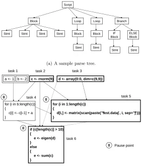
2.5
Ease of Use Demonstration
… u<-TRUE la<-list()
for (i in 1:length(l)) la[[i]]<-attributes(l[[i]]) o<-la[[1]]
if (o$type=="factor") { o<-o[names(o)!="levels"] }
o<-o[names(o)!="type"] o<-o[names(o)!="dimnames"] …
library(Rmpi) library(snow) …
cl <- makeCluster(4, type = “MPI”) u<-TRUE
la<-clusterApply(cl,l,attributes) o<-la[[1]]
if (o$type=="factor") { o<-o[names(o)!="levels"] }
o<-o[names(o)!="type"] o<-o[names(o)!="dimnames"] stopCluster(cl)
…
Figure 2.5: Comparison with the snow package interface
These two codes perform the same R operations and generate the same results.
Statements that call snow APIs are printed in italic. With snow, users must first include both the RMPI and the snow libraries, then explicitly create a “cluster” consisting of four processors using makeCluster. The user then executes the function attributes
on the elements of the target list lin parallel on this cluster using clusterApply. In this case the results will be stored as the elements of the listla. Finally the user has to remove the cluster by calling stopCluster. In addition, snow has inconvenient restrictions with parallel interfaces like clusterApply. For example, here the list l is allowed to have at most as many elements as the number of nodes in the cluster.
The sequential version on the left side, however, carries out the attributes oper-ations in a loop, as typically will be done to perform such a task. With pR, this sequential version can be automatically parallelized without any modification as an ordinary MPI job. Suppose an script is stored in file example.R, the regular command to execute it in batch mode with R is
R CMD BATCH example.R,
then the command to execute it in parallel with pR is simply
mpirun -np <num procs> pR example.R
This allows a sequential code to run unmodified, a feature not yet provided by any existing parallel scripting language environments.
in the sequential script must be stored in the shared file system and appropriate paths are provided in the code.
2.6
Performance Evaluation
Our experiments were performed on theopt64cluster located at NCSU, which has 16 2-way SMP nodes, each with two dual-core AMD Opteron 265 processors. The nodes have 2GB memory each and are connected using Gigabit Ethernet and run Fedora Core 5. A single NFS server manages 750GB of shared RAID storage.
We performed each test multiple times and observed that the performance variance was very small (with standard deviations less than 6%), so error bars were omitted.
0 5 10 15 20 25 30 32 16 8 4 2 1 Speedup
Number of Processors pR pR-ideal (a) 0 5 10 15 20 25 30 35 32 16 8 4 2 1 Speedup
Number of Processors pR
pR-ideal
(b)
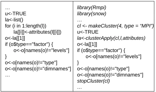
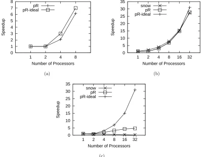
Figure 2.6: Performance of pR with various benchmarks. Error bars are omitted since variances are small. The average 95% confidence interval (CI) of pR is 0.98% and maximum 95% CI is 2.86%. (a) Performance with the synthetic loop code. (b) Performance with the Boost application.
2.6.1 Synthetic Loop
snow interface here. In order to use snow, all the functions inside the iteration have to be wrapped up into one function and passed as a parameter to the snow interface. pR avoids this additional step and provides totally transparent parallelization.
Figure 2.6(a) illustrates the performance of pR with the above small synthetic R code on 2 to 32 processors, with the “1 processor” data point marking the sequential running time in the native R environment. We also plot the ideal speedup for pR, which grows linearly with the number of workers (note that the master does not carry out any heavy-weight computation). For example, with 8 processors the ideal speedup is 7. The speedup of pR follows closely the ideal speedup up to 8 processors. When we use 16 processors or more, the hardware contention on the SMP nodes and the unevenly distributed number of iterations are the major reasons for the gap between the pR and the ideal speedup.
2.6.2 Boost
Now we evaluate pR using two real applications. The first application is Boost, a real-world application acquired from the Statistics Department at NCSU. This code is a simulation study evaluating an in-house boosting algorithm for the nonlinear transforma-tion model with censored survival data. The nonlinear transformatransforma-tion model is complex, and the boosting algorithm is computationally intensive. Moreover, the simulation study often requires a large number of repeated data generation and model fitting, and the total computational time can be forbidding.
The bulk of computation in Boost is spent on a loop, which contains other loops. The only modification we made to Boost before running it in pR is to change the number of iterations in one inner loop (which is not parallelized) to reduce the execution time, as the original code runs for dozens of hours.
is mainly due to the fact that the contention between the two processors on each SMP node, as the computation speedup (the speedup in executing Boost’s main loop) drops to around 1.5 from 16 to 32 processors. Meanwhile, the pR overhead also increases when both processors on a node are used.
0 1 2 3 4 5 6 7 8 8 4 2 1 Speedup
Number of Processors pR pR-ideal (a) 0 5 10 15 20 25 30 35 32 16 8 4 2 1 Speedup
Number of Processors snow pR pR-ideal (b) 0 5 10 15 20 25 30 35 32 16 8 4 2 1 Speedup
Number of Processors snow
pR pR-ideal
(c)
Figure 2.7: Performance of pR with various benchmarks. Error bars are omitted since variances are small. The average 95% confidence interval (CI) of pR is 0.98% and maximum 95% CI is 2.86%. The average 95% CI of snow is 1.44% and maximum 95% CI is 5.63%. (a) Performance with the sensor network code. (b) Performance with the bootstrap code. (c) Performance with the SVD code.
2.6.3 Sensor Network Code
due to failure or suppression (when a reading is not sent on purpose because it hasn’t changed). Normally, it is impossible to distinguish a failure from suppression. Low-cost redundancy is added to transmitted messages to help identify when failures and suppres-sions have occurred, and that information is used to constrain Bayesian inference of the missing values [109]. The main body of this sensor network R code consists of a loop of 8 iterations, which makes up the bulk of its computation. Each iteration performs statistical analysis on different input data and calls several computation-intensive functions. The loop is embarrassingly parallel in nature and therefore ideal for parallelization.
Figure 2.7(a) shows the speedup of running the sensor network code with pR. Since the loop has only 8 iterations, we use up to 8 processors. The speedup achieved using pR is decent, reaching 6.15 with 8 processors total. The gap between the pR curve and the ideal speedup curve is due to two factors. First, the independent iterations are not able to be evenly distributed to the workers. Second, the execution time of each iteration varies from 32 to 138 seconds depending on input data.
2.6.4 Bootstrap
Next, we compare pR’s performance with that of the snow package. We select two representative synthetic test cases here.
The first test case was the bootstrap example taken from an online snow tuto-rial [116]. It performs bootstrap in a loop using the R boot function and the nuclear data provided in R. This forms an ideal case for parallelization, as it is computation-intensive but not data-intensive. We created the corresponding sequential code using a for loop. Figure 2.7(b) portraits the performance of snow and pR.
2.6.5 SVD
The second synthetic test case performs SVD on each 2-D slice in a large 3-D array. In this case, the initialized array must be partitioned and distributed to all the workers, while the results must be gathered. This code is both computation- and data-intensive.
Figure 2.7(c) shows that the speedup achieved by pR is significantly worse than the ideal value. The parallel performance saturates beyond 16 processors and peaks around 4.7. Still, this performance is over an order of magnitude better than snow’s, which never produces any speedup starting from 2 processors and actually slows down the application by over 4 times with 16 and 32. This behavior is consistent with what the snow authors reported with communication-intensive codes [101].
For data to be communicated between processes and interpreted correctly as R objects, both snow and pR uses the serialization function provided by R which can write an R object to a scalar string. This helps to keep the parallelization package high-level and easy to work with R updates. However, we have found through our measurement that the R serialization can be more costly than the inter-processor communication. To verify this, we benchmarked the point-to-point MPI communication time and the R serialization time of an 8MB array. On our test cluster, we measured the MPI bandwidth to be 72.5MB/s, while the R serialization bandwidth is only 1.9MB/s. In pR, since the array initialization func-tion call is treated as one task, one worker performs this initializafunc-tion, serializes partifunc-tions of the array, and sends these partitions to the appropriate workers. Therefore the array initialization time remains constant and the communication time increases as the number of workers grows. Such overhead becomes more dominating as more workers are used and the parallel R task execution time shrinks.
The reason that pR’s performance is much better than snow, we suspect, is due to the fact that pR is implemented in C and directly issues MPI calls. In contrast, snow is implemented in R itself and calls R’s high-level functions for message passing, which may result in worse communication performance.
2.6.6 Overhead Analysis
Table 2.1: Itemized overhead with the Boost code, in percentage of the total execution time. The sequential execution time of Boost is 2070.7 seconds.
2 4 8 16 32
Initialization 0.05 0.13 0.31 0.65 1.28 Analysis 0.00 0.00 0.00 0.01 0.04 Master MPI 0.00 0.00 0.00 0.00 0.01 Max wkr. serial. 0.42 0.69 1.15 2.05 3.19 Max wkr MPI 0.00 0.03 0.07 0.15 0.26 Max wkr socket 0.01 0.01 0.02 0.04 0.05
Table 2.2: Itemized overhead with the sensor network code, in percentage of the total execution time. The sequential execution time is 825.2 seconds.
2 4 8
Initialization 0.09 0.23 0.52 Analysis 0.00 0.01 0.01 Master MPI 0.00 0.00 0.00 Max wkr. serial. 0.00 0.00 0.01 Max wkr MPI 0.00 0.00 0.00 Max wkr socket 0.00 0.00 0.00
is spent on this particular category of overhead.
We measure six types of pR overhead. “Initialization” includes the cost of initializ-ing the master and the worker processes, performinitializ-ing the initial communication, and loadinitializ-ing necessary libraries. “Analysis” includes the total dependence analysis time. “Master MPI” is the sum of time spent on message passing after the initialization phase on the master node. The next three categories stand for the data serialization, inter-node communication
Table 2.3: Itemized overhead with the bootstrap code, in percentage of the total execution time. The sequential execution time of bootstrap is 2918.2 seconds.
2 4 8 16 32
The sequential execution time of SVD is 227.1 seconds.
2 4 8 16 32
Initialization 0.23 0.49 0.78 1.12 1.27 Analysis 0.00 0.00 0.00 0.01 0.02 Master MPI 0.00 0.00 0.00 0.00 0.01 Max wkr serial. 11.70 26.46 41.71 52.98 57.98
Max wkr MPI 0.00 2.10 4.32 6.44 7.83 Max wkr socket 1.45 1.56 1.99 2.40 2.51
(MPI), and intra-node communication (socket), respectively. For each category, we sum up the total overhead on each worker, and then report the maximum value across all the workers.
The first observation we can draw here is that analysis overhead is very insignifi-cant, counting for less than 0.005% in most cases. The slight increase in the relative cost of analysis as more workers are used is more due to the decrease of the overall execution time. Initialization, on the other hand, steadily increases with the number of workers, because this process involves loading libraries at the workers. This overhead grows as the I/O contention increases, especially with the NFS server equipped at our test cluster. The initialization cost also varies from application to application. Note that the SVD code has a very small initialization cost since it does not load extra libraries. This is not reflected directly in the tables as SVD’s execution time is much shorter than the other two test cases. After the initialization phase, the master has little MPI communication overhead, since most of the inter-processor data communication happens between the workers.
The worker-side overhead heavily relies on how data-intensive an application is. For bootstrap, there is almost no data communication between workers, and we measured minimal worker communication overheads. In contrast, with SVD such overheads may dominate the total execution time. With 32 processors, the SVD code spends 58% of the total execution time on data serialization, and a total of around 10% on data communication. This explains the small speedup we observed in Figure 2.7(c).
2.6.7 Task Parallelism Test
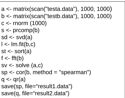
a <- matrix(scan("testa.data"), 1000, 1000)
b <- matrix(scan("testb.data"), 1000, 1000) c <- rnorm (1000)
s <- prcomp(b) sd <- svd(a) l <- lm.fit(b,c) st <- sort(a) f <- fft(b) sv <- solve (a,c)
sp <- cor(b, method = "spearman") q <- qr(a)
save(sp, file=“result1.data”) save(q, file=“result2.data”)
Figure 2.8: The task parallelism test code
Finally, we use another synthetic test case to test pR’s capability of parallelizing non-loop tasks. Figure 2.8 lists the source code. The first three statements read two 2-D matrices from two separate input files, and create a vector with normal distribution. Following those are 8 R function calls that perform a variety of tasks on one or more of these data objects. These tasks include principal components analysis (prcomp), SVD (svd), linear model fitting (lm.fit), variance computation (cor), sorting (sort), FFT (fft), equation solving (solve), and QR decomposition (qr). Finally, a subset of results are written back to two output files. The sequential running times of these tasks range from less than 3 seconds for most of them, to 19 seconds for SVD and 27 seconds for the linear model fitting. The total sequential time spent on the three data object initialization statements is around 3 seconds.
Table 2.5: The parallel execution time and speedup of the task parallelism test script
1 2 4 8
Exec time 90.37 122.26 49.37 35.82
Speedup 1 0.74 1.83 2.52
the worker front-end process adds significant overhead. This causes the overall execution time to grow by 35%. With more processors, the parallel execution performance picks up and pR achieves a speedup of 2.5 with 8 processors. Considering that the longest execution path (including the initialization of b and c, and the lm.fit call) costs 30.1 seconds, the total execution time with 8 processors at 35.82 seconds is reasonable given the known high expense of the R serialization.
This sample test also demonstrates file dependence analysis and parallel file op-erations. With the runtime file dependence check turned on and pR used system calls to examine inodes, the total analysis cost was indeed considerably increased, by 81%, from 0.0036 to 0.0066 second. Still, the absolute cost of making the four file operation checks are quite small. The two input operations using scan are scheduled at almost the same time when 4 or more processors are used, and in this case the total execution time of these two tasks is reduced from 2.4 to around 2 seconds. Consider our test cluster uses a single NFS server, we expect to see larger benefit of parallelizing I/O operations on platforms with parallel file system support.
2.7
Summary
Scripting languages such as R and Matlab are widely used in scientific data pro-cessing. As the data volume and the complexity of analysis tasks both grow, sequential data processing using these tools often becomes the bottleneck in scientific workflows. We pro-pose pR, a runtime framework for automatic and transparent parallelization of the popular R language used in statistical computing.
Chapter 3
Autonomic Task Scheduling
In Chapter 2 we have presented and built a transparent framework for parallel data processing. However, one key issue we have not sufficiently addressed in this transparent framework is task scheduling. There have been numerous studies of task scheduling in parallel processing, applying to various scenarios and constraints. Data processing tools written in scripting languages such as R often exhibit multi-level of parallelism, which usually remain unexploited. This brings new opportunity for task scheduling.
In this chapter, we discuss optimization techniques with respect to task partition-ing and schedulpartition-ing. We first illustrate the problem and the opportunity uspartition-ing an example R script. In the rest this chapter, we present several techniques developed in this thesis study, including using Artificial Neural Networks for runtime task cost prediction and ex-tending an existing static scheduling algorithm. We then discuss our evaluation methods and present experiment results.
3.1
Motivation
a <- array(rnorm(1200*1200), dim=c(1200, 1200)) 1
b <- list() 2
c <- array(rnorm(1200*1200), dim=c(1200, 1200)) 3
f <- friedman.test(a) 4
w <- wilcox.test(c) 5
for (i in 1 : 1200) { 6
b[[ i ]] = mean( c %% a[i, ]) 7
} 8
L: T1: T2:
Figure 3.1: A sample R script
T1 T2 L3 L4 L5 L6 L7
L2 L1
L8 T1 T2 L3 L4 L6 L7 L8
Processor
0 1 2 3 4 5 6 7 0 1 2 3 4 5 6 7
T
im
e
(a) Imbalanced schedule
L8 T1 T2 L3 L4 L6 L7 L8
L2 L1
L5
0 1 2 3 4 5 6 7 0 1 2 3 4 5 6 7
Processor
T
im
e
(b) Balanced schedule
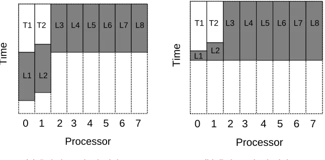
Figure 3.2: A motivating example with sample schedules that show task lengths proportional to their execution time on an eight core system
be executed in parallel. Further, there are no dependences between the iterations of L so they can also be parallelized. However, a straightforward loop decomposition and task distribution will not produce an efficient parallel execution schedule, as demonstrated by the example schedules that use lengths proportional to the execution times for L, T1 and T2 on an eight core system. Figure 3.2(a) shows a naive schedule that divides L iterations evenly by the number of processors. Since the functions and the loop blocks execute whenever a processor is available, two loop blocks use the same processors as T1 and T2. Thus, this schedule leaves six processors idle while those loop blocks complete. In contrast, Figure 3.2(b) shows a much more desirable schedule that optimizes the loop decomposition in light of the tasks to provide perfect load balance, but requires an accurate prediction of all tasks’ execution times before scheduling L.
our goal is an implicit parallelization mechanism, we must use transparent performance models that predict those costs. We achieve this by observing the performance of appli-cation components and then using the collected information to predict later executions of those components. This approach particularly suits scripting languages since they typically have a small set of functions (often with relatively stable parameter ranges) that are used repeatedly both within a single job and across jobs, whether belonging to the same user or not. Thus, we can gather enough samples, potentially from multiple jobs or even from multiple users in a shared performance data repository, for accurate predictions.
We present our novel runtime parallelization tool that performs intelligent loop decomposition and task scheduling, based on performance models derived from past per-formance data collected on the local platform. We use artificial neural networks (ANNs), which are application-independent and self-learning black box models, as required for im-plicit parallelization. We integrate these techniques into the existing pR framework [74], which performs runtime, automatic parallelization of R scripts. The result is an adap-tive scheduling framework for the parallel execution of R, which we call ASpR (Adapadap-tively Scheduled parallel R).
For the example in Figure 3.1, ASpR now estimates the costs of T1 and T2 based on past calls to those functions. Further, it can infer the cost of the individual iterations of L based on the early feedback collected by “test driving” the same loop. We then use these cost estimates as inputs for our scheduling algorithm, which is an extension of MCP scheduling algorithm [121] to generate an informed loop partitioning and scheduling plan that is close to the one shown in Figure 3.2(b).
3.2
Background on Artificial Neural Networks
Artificial Neural Networks (ANNs) are machine learning models based on bio-logical neural networks. ANNs have been designed as a powerful and automatic method for solving a variety of problems including pattern recognition, clustering, prediction and forecasting [60].
..
.
..
.
..
.
Input
Layer
Hidden
Layer
Output
Layer
Input 1
Input 2 Input 3
Input n
Output 1
Output m
Figure 3.3: A sample feed-forward neural network
Typical ANNs have a connected, feed-forward network architecture with an input layer, one or morehidden layers, and anoutput layer, as is shown in Figure 3.3. Each layer consists of a set of neurons that are each connected to all neurons in the previous layer. Input values are fed into the input layer, with computation passing through the hidden layer(s) and finally predictions are extracted from the output layer. Each neuron computes its output by applying an activation function to a weighted sum of its inputs. Different types of activation functions involve a threshold function, a piecewise linear function, a sigmoid function, and a Gaussian function. Figure 3.4 shows an example of neuron in the hidden layer with a sigmoid activation function.
Figure 3.4: A sample hidden layer unit with a sigmoid activation function (borrowed from [81])
3.3
ASpR System Architecture
Although we propose a general purpose approach, we present our new Adaptively Scheduled parallel R (ASpR – pronounced “aspire”) framework within the context of our test platform, the pR framework [74] for transparent R script execution [96]. pR takes a sequential R script as input and transparently executes it in parallel using a master-worker model. The master parses the input script, conducts dependence analysis, and schedules non-trivial tasks(function calls and loop blocks) to the workers, where they are computed in parallel. The workers are assigned these tasks and carry out communication to exchange task information with the master, as well as data communication among themselves. Cur-rently pR does not further parallelize the content of function calls or loops, and with nested loops only the outermost loop is parallelized. Only the underlying framework imposes these restrictions. Our concepts introduced in this work do not require them and can be applied to systems with hierarchical parallelization without major modifications.
In our proposed approach, ASpR, we extended the intelligence within the pR mas-ter to include three new modules, as illustrated in Figure 3.5: (1) the analyzer, which performs dependence analysis as well as parsing the R scripts and generates a Task Prece-dence Graph (TPG); (2) the performance modeler, which predicts task computation costs and data communication costs for the TPG; and (3) the DAG scheduler, which determines an appropriate schedule through a static algorithm that uses the cost predictions from the performance modeler as input and dispatches the tasks to workers accordingly.
DAG Scheduler Analyzer . . . Master DAG Task Precedence Graph R Scripts Worker 2 Worker 1 Worker n Performance Modeler ANN Model .. . ... .. . Performance Data Repository sliding window buffer
… … Training Q u e ry P re d ic tio n s Loop
Test Driving Performance
Figure 3.5: Adaptively Scheduled parallel R (ASpR) architecture overview
is that each individual user often uses a limited set of functions, standard or user-defined, which tend to be called repeatedly in this user’s scripts. The functions can be easily identi-fied by their function names, though the calls to the same function may likely use different input parameters. Loops, on the other hand, are harder to identify but often have stable per-iteration cost in data processing scripts. Therefore, the performance modeler employs a light-weight performance data repository and adopts machine-learning methods to model and predict function task costs. For loops, it takes a more straight-forward approach by “test-driving” the initial iteration to give the per-iteration loop execution cost based on actual measurement.
A file-based performance repository collects the local script execution history for function cost prediction. We retrain the performance model as new performance data become available. To reduce the performance modeling overhead, a sliding window buffer is allocated to store the most recent data points. When applied to systems adopting the master-worker paradigm, such as pR, the system overlaps retraining with script execution on the workers resulting in low training overhead.