Low Complexity Bit-Parallel Square Root
Computation over
GF(
2
m
) for all Trinomials
∗
Francisco Rodr´ıguez-Henr´ıquez, Guillermo Morales-Luna
Computer Science Section
CINVESTAV-IPN
Av. IPN 2508, Mexico City, Mexico
{
francisco, gmorales
}
@cs.cinvestav.mx
Julio L´opez-Hern´andez
Institute of Computing
State University of Campinas, Brazil
[email protected]
Abstract
In this contribution we introduce a low-complexity bit-parallel algo-rithm for computing square roots over binary extension fields. Our pro-posed method can be applied for any type of irreducible polynomials. We derive explicit formulae for the space and time complexities associated to the square root operator when working with binary extension fields gener-ated using irreducible trinomials. We show that for those finite fields, it is possible to compute the square root of an arbitrary field element with equal or better hardware efficiency than the one associated to the field squaring operation. Furthermore, a practical application of the square root operator in the domain of field exponentiation computation is presented. It is shown that by using as building blocks squarers, multipliers and square root blocks, a parallel version of the classical square-and-multiply exponentiation algo-rithm can be obtained. A hardware implementation of that parallel version may provide a speedup of up to 50% percent when compared with the tradi-tional version.
keyword: Finite field arithmetic; binary extension fields; cryptography
1 Introduction
Arithmetic over binary extension fieldsGF(2m) has many important applications, particularly in the theory of error control coding, symmetric block ciphers and elliptic curve cryptosystems [1,2,3,4,5]. Those applications typically require high performance implementation of most if not all of the basic finite field operations such as field addition, subtraction, multiplication, division, exponentiation and square root [6].
In particular, field square root computation has become an important building block in the design of some elliptic curve primitives such as point compression and point halving [1,3,4]. Moreover, recently, a novel parallel formulation of the standard Itoh-Tsujii multiplicative inverse algorithm for multiplicative inverse computation overGF(2m) using as main building blocks field multiplication, field squaring and field square root operators was proposed in [7]. A speedup of nearly 30% with respect to the original Itoh-Tsuii was reported.
For most applications, the efficiency of finite field arithmetic implemented in hardware is typically measured in terms of associated design space and time complexities. The space complexity is defined as the total amount of hardware resources needed to implement the circuit, i.e. the total number of logic gates required by the design. Time complexity, on the other hand, is simply defined as the total gate delay or critical path of the circuit, frequently formulated using gate delayTxunits.
Let P(x) be an irreducible polynomial overGF(2). Then, the binary extension field of degreem∈N+GF(2m)can be defined as,
GF(2m)∼=GF(2)[x]/(P(x)) =©a
0+a1x+· · ·+am−1xm−1 modP(x)|ai ∈GF(2) ª
Field square root operation is defined as follows. LetAbe an arbitrary element in the fieldGF(2m)as described above. The square root ofA, denoted as√Aor A12, is the elementD∈GF(2m)such thatD2 =AmodP(x).
A straightforward but rather expensive approach for computing√A is based on Fermat’s Little Theorem which establishes that for any nonzero element A ∈
GF(2m), the identityA2m
= Aholds. Therefore,√Amay be computed asD = A2m−1
A more efficient algorithm based on a refining of the above Fermat’s Little Theorem method was proposed by Fong et al. in [8,9], and it is based on the ob-servation that√Acan be efficiently implemented by extracting the two half-length vectorsAeven = (am−1, am−3,· · · , a2, a0) andAodd = (am−2, am−4,· · · , a3, a1)
and by performing a field multiplication of length bm
2c of Aodd with the pre-computed value of the elementx12 followed by an addition withAeven. The cost
of the algorithm presented in [8] consists of one field multiplication of lengthm/2 bits by a pre-computed constant, which is still an expensive operation.
However, if the irreducible polynomialP(x)is a trinomial,P(x) = xm+xn+ 1withman odd prime number. The authors in [8] observed that the square root of any arbitrary elementA∈GF(2m) can be computed using relatively few additions and shift operations. In particular, in [8] is reported that the computational cost of a square root in the fieldGF(2233), usingP(x) = x233+x74+ 1, requires roughly 1/8the time of a field multiplication when both operations are implemented in a software platform.
In this contribution, an alternative method for computing square roots over binary finite field is proposed. The most important findings presented in this paper are threefold. Firstly, after a careful analysis of the method proposed in [8], we derive a closed expression for the square root operator when using irre-ducible trinomials of the type P(x) = xm +xn + 1, with m odd, n even, and
dm−1
4 e ≤ n < b m−1
3 c. Secondly, we describe an alternative method for com-puting √Awhich is based on the linear property exhibited by the field squaring operation in binary extension fields. Our proposed method can be applied for any type of irreducible polynomials. In particular, it is shown that for the important practical case of finite fields generated using irreducible trinomials, the square root operation can be performed with no more computational cost than the one associated to the field squaring operation. Moreover, we derive explicit formulae for both, field squaring and square root operations, detailing their corresponding area and time complexities when implemented in hardware platforms. Thirdly, we present a practical application of the square root operator in the domain of field exponentiation computation.
The rest of this paper is organized as follows. Section2provides an analysis of the method proposed in [8]. Furthermore, a closed expression for the square root operator when using irreducible trinomials of the typeP(x) =xm+xn+ 1, withmodd,neven, anddm−1
4 e ≤n <b m−1
proposed bit-parallel algorithm for square root computation is explained in detail. Moreover, we give explicit formulae for the efficient computation of squaring and square roots over binary extension fields generated by irreducible trinomials. Section5includes several illustrative examples of field square root computation. Section6 describes how the square root operator can be applied for speeding up the exponentiation operation in binary extension fields. Finally, in Section7some conclusion remarks are drawn.
2
The Fong et al. Method for Computing Square
Roots
As it was mentioned in the previous Section, the Fong et al. method for comput-ing square roots over binary extension fields is based on the observation that the element√Acan be expressed in terms of the square root of the monomialxas,
A12 =
m−1 2
X i=0
a2ixi+x12
m−3 2
X i=0
a2i+1xi modP(x) (1)
Eq. (1) can be efficiently implemented by extracting the two half-length vec-torsAeven = (am−1, am−3,· · ·, a2, a0)andAodd = (am−2, am−4,· · · , a3, a1)and by performing a field multiplication of lengthbm
2cofAodd with the precomputed valuex12 followed by an addition withAeven.
In the event that the irreducible polynomialP(x)is a trinomial,P(x) = xm+ xn + 1 with m an odd prime number, authors in [8] found the following handy equations for√A,
A12 =
(
Aeven+ (x
m+1 2 +x
n+1
2 )·Aodd nodd,
Aeven+ h
x−m−1
2 (xn2 + 1)·Aodd
i
modP(x) neven. (2)
According to Eq. (2), when the middle coefficientn of the irreducible trinomial P(x)is odd, the square root of any arbitrary element A ∈GF(2m) can be found using few additions and shift operations 1. However, in the case that the middle
coefficient n is even, the square root computation becomes a bit more computa-tional intensive. In the following we analyze the latter case in more detail.
1We stress that the polynomial(xm+1 2 +x
n+1
2 )·Aoddhas degreem−1. Thus, in this case we
Notice that in the quotient fieldGF(2)[x]/(P(x)), isomorphic toGF(2m), the elementx−m2−1 can be computed by using the reduced identityx−s =xn−s+xm−s, for 1 ≤ s ≤ n. If we impose now the restrictiondm−1
4 e ≤ n ≤ m−21, it follows that m−1
2 <2n. Then, in the fieldGF(2)[x]/(P(x))we can write,x−n = 1+xm−n and lettingt= m−1
2 −nwe have the following identities moduloP(x): x−t=xn−t+xm−t=x2n−m−21 +xn+m2+1
Then, the elementx−m−21 =x−t·x−ncan be written as, x−m2−1 = x−t·x−n
= (x2n−m−21 +xn+m2+1)·(1 +xm−n) = x2n−m−21 +xn+
m+1
2 +xn+
m+1
2 +xm+
m+1 2
Therefore,
x−m−1
2 (xn2 + 1) =x2n−m2−1 +xm+12 +x2n+2m+1 +x
5n−(m−1)
2 +xm+2n+1 +x3n+2m+1
After examining above equation, it results convenient to impose an additional restriction to the middle coefficientn, namely,n <bm−1
3 c. In this way, we assure that the exponent 3n+m+1
2 will not exceed the valuem.
Above result and Eq. (2) indicate us how to calculate the square root of an arbitrary nonzero field element A ∈ GF(2m), when the field has been generated using the irreducible trinomialP(x) =xm+xn+ 1, withman odd number and n an even number such thatdm−1
4 e ≤ n < bm3−1c. The explicit formula is given as,
A12 = Aeven+
Aodd ³
x2n−m−21 +xm2+1 +x2n+2m+1+
x5n−(2m−1) +x
m+n+1 2 +x
3n+m+1 2
´
. (3)
In the following Sections we will discuss alternative methods for deriving and developing even further Eqs. (2) and (3).
3 A Linear Algebra Analysis of the Squaring and
Square Root Field Operations
field GF(2m) is equivalent to the quotient fieldGF(2)[x]/(P(x)). Thus in what follows all polynomial identities shall be understood modulo P(x). Then, in the fieldGF(2m)the followingReduction Ruleholds:
k ≥m =⇒ xk =xk−mxm =xk−m(1 +xn) = xk−m+xk−m+n, (4)
in other words, the powerxkcan be expressed as the addition of two lower powers whose exponents differ inn.
LetAbe an arbitrary element of the fieldGF(2m), represented in the canonical basis as anm−1degree polynomial, namely,
A(x) = mX−1
i=0
aixi , ai ∈0,1, 0≤i≤m−1.
Then the square C = A2 modP(x)in GF(2m) may be obtained by computing first the polynomial product ofA by itself, followed by a reduction step modulo P(x). In fact, since the characteristic of the field is 2, the square map is linear, thus the polynomial square ofAis,
A2(x) = Ã
mX−1 i=0
aixi !
·
à mX−1
i=0 aixi
! =
mX−1 i=0
aix2i (5)
Let X1 = [1x · · · xm−1]T be the m-dimensional column vector whose entries are the consecutive powers of x. Since squaring is linear and its kernel contains only the element0∈GF(2m), the set of squares{x2i}m−1
i=0 is linearly independent, thus it forms a basis of GF(2m). LetX
2 = £
1x2 · · · x2(m−1)¤T be the column vector whose entries are the elements of that basis. Then, there is a non-singular (m×m)-matrixN we haveX2 =NX1. The matrixN can be partitioned as
N = ·
L0 K0
¸
(6)
whereL0is a matrix of orderm1×m,K0is a matrix of orderm2×m,m1 =dm2e, m2 =m−m1, and the rows ofL0 are the canonical vectors with even indexes:
L0 = [`ij]00≤≤ij≤≤mm1−−11 and (`ij = 1 ⇐⇒ j = 2i). (7)
Furthermore, for2i ≥ m, let us writer = 2i−m. Then, from the reduction rule (4), we havex2i = xr+xn+r. Notice that whenever the second exponent of last expression is not lower thanm, the reduction rule may be reapplied.
Thus, the first rows, namelybm/2c − bn/2c, ofK0have just two values 1 and they are at entries whose separation isn. Eq. (5) asserts that, with respect to the polynomial basis, the column vector consisting of the coordinates, with respect to the polynomial basis, ofA2 is given as,
c=NTa (8)
whereais the coefficient vector ofA.
Naturally, the inverse of NT will represent the square root linear map, with respect to the polynomial basis. Let us calculate the inverse matrixN−1ofN. As we did in Eq. (6), let us introduce the following partition
N−1 = [ L
1 K1 ] (9)
whereL1has orderm×m1,K1has orderm×m2,m1 =dm2eandm2 =m−m1. From (6) and (9) we get,
1m =N N−1 = ·
L0 K0
¸
[L1 K1 ] = ·
L0L1 L0K1 K0L1 K0K1
¸
where1mis the(m×m)-identity matrix. From above equations, it follows that,
1m1 =L0L1 , 0m2×m1 =K0L1 (10)
0m1×m2 =L0K1 , 1m2 =K0K1. (11)
Eqs. (10) assert that the columns ofL1 should, on the one hand, form a biortho-normal system with the rows of L0, and, on the other, be orthogonal to the rows ofK0.
We observe that the rows ofL0 form an orthonormal basis of a space S0 of dimension m1 over GF(2m) considered as them-dimensional vector space over the prime fieldGF(2). Thus the orthogonal complement ofS0 has dimensionm2. In other words, there are exactly2m2 vectors which are orthogonal to all rows in
L0. Hence, there exist2m1m2 matricesLof orderm×m1such thatL0L=0m1.
Due to the special form of L0, if the even-indexed rows of a matrix L are selected, a zero matrix is gotten. LetL⊥
Also we haveL0LT
0 =1m1. It follows that the general solution of the first equation
in (10) is given as,
L1 =LT0 +L withL∈L⊥0. (12) In order to satisfy the second equation in (10) we must have
K0LT0 =K0L. (13)
Let us write K0 = (kij)00≤≤ij≤≤mm2−−11. From relation (7), it follows that the general entry ofK0LT
0 is
Pm−1
µ=0 kiµ`jµ =ki,2j, for0≤i≤m2−1,0≤j ≤m1−1. Equation (13) will be satisfied if and only if the inner product of thei-th row of K0and thej-th column ofLgives the valueki,2j,0≤i≤m2−1,0≤j ≤m1−1. Hence, matrixK0 should satisfy the following conditions:
ki,2j = 0 =⇒ µ
there is an even number of 1’s in the i-th row of K0 appearing at odd indexed entries
¶ (14)
ki,2j = 1 =⇒ ∃ji odd:ki,ji = 1 (15)
Conditions (14) and (15) along with the fact that the matrix N is non-singular, determine uniquely the matrix L ∈ L⊥
0. As a consequence, the submatrix L1 that satisfies eqs. (10) is also uniquely determined. In a similar but more compli-cated way, it can be verified that the submatrixK1satisfying eqs. (11) is uniquely determined.
Based on the conclusions obtained from the linear algebra approach just out-lined, we derive in the next Section explicit formulae for the field square root operation.
4 Explicit Formulae for the Squaring and Square
Root Field Operations
Once again, let us consider binary extension fields constructed using irreducible trinomials of the form P(x) = xm +xn+ 1, with m ≥ 2. It is convenient to consider, without loss of generality, the additional restriction1≤n ≤ bm
2c2.
2It is known that ifP(x) = xm+xn + 1is irreducible overGF(2), so isP(x) = xm+
xm−n+ 1[10]. Hence, provided that at least one irreducible trinomial of degreemexists, it is
always possible to find another irreducible trinomial such that its middle coefficientnsatisfies the restriction1≤n≤ bm
The rest of this Section is organized as follows. First, in Subsection 4.1, we give the corresponding formulae needed for computing the field squaring opera-tion when considering arbitrary irreducible trinomials. Those equaopera-tions are then used in Subsection 4.2 to find the corresponding ones for the field square root operator.
4.1 Field Squaring Computation
Let A = Pmi=0−1aixi be an arbitrary element of GF(2m). Then, according to Eq. (5) its square,A2, can be represented by the2m-coefficient vector,
A2(x) = £0 a
m−1 0 am−2 . . . 0 a1 0 a0 ¤ = £a0
2m−1 a0m−2 . . . a0m−1 am0 ; a0m−1 a02 . . . a01 a00 ¤
(16)
wherea0
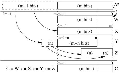
i = 0foriodd. Let us reduce this vector using rule (4). Hence, the upper half ofA2 (i.e., themmost significant bits) in Eq. (16) is mapped into the firstm coordinates by performing addition and shift operations only. Let us write
C = A2 modP(x) = A0
[0,m−1]+A0[m,2m−1]+A0[m,2m−1−n]xn +¡A0
[2m−n,2m−1]+A0[2m−n,2m−1]xn ¢
(17) Thus, the reduction step is computed by the addition of four terms,
W = A0[0,m−1] X = A0[m,2m−1]
Y = A0
[m,2m−1−n]xn Z = A0
[2m−n,2m−1]+A0[2m−n,2m−1]xn
This procedure is shown schematically in Fig.1. Notice that for those designs im-plemented in hardware platforms, the field squaring computation procedure just outlined can be instrumented by using XOR logic gates only. Nevertheless, the ex-act computational complexity of this arithmetic operation depends on the explicit form ofmand the middle coefficientnin the trinomialP(x).
(m−1 bits) (m bits) m−1 0 2m−1 m Z (m bits) 2m−1 m−1−n n (m bits) (m−n bits) (n) (n) (n) X Y m−1 0
(m bits) C C = W xor X xor Y xor Z
m
W A²
Figure 1: Reduction scheme.
Type I: ComputingC = A2 modP(x), withP(x) = xm+xn + 1, meven, n odd andn < m
2, ci = ai
2 +a
m+i
2 ieven,i < nori≥2n,
ai
2 +a
m+i
2 +am−n+
i
2 ieven,n < i <2n,
am+1−n+i
2 iodd,i < n,
am−n+i
2 iodd,i≥n,
(18)
fori = 0,1,· · · , m−1. It can be verified that Eq. (18) has an associated cost of m+n−1
2 XOR gates and2Tx delays.
Type II: ComputingC =A2 modP(x), withP(x) =xm+xn+ 1,meven, nodd andn= m
2,
ci = ai
2 +am2+i ieven,i < n,
ai
2 ieven,i > n,
am+1−n+i
2 iodd,i < n,
an+i
2 iodd,i≥n,
(19)
fori = 0,1,· · · , m−1. It can be verified that Eq. (19) has an associated cost of m+2
4 XOR gates and oneTx delay.
numbers andn < m+1 2 ,
ci = ai
2 ieven,i < n,
ai
2 +a
i
2+
m−n
2 +a
i
2+(m−n) ieven,n < i <2n,
ai
2 +a2i+
m−n
2 ieven,i≥2n,
am+i
2 +a
m+i
2 +
m−n
2 iodd,i < n,
am+i
2 iodd,i≥n,
(20)
fori = 0,1,· · · , m−1. It can be verified that Eq. (20) has an associated cost of m−1
2 XOR gates and2Txdelays.
Type IV: ComputingC = A2 modP(x), withP(x) = xm+xn+ 1, modd, n even andn < m+1
2 , ci = ai
2 +a2i+m−n2 ieven,i < n,
ai
2 +a
i
2+m−n ieven,n≤i <2n,
ai
2 ieven,i≥2n,
am+i
2 iodd,i < n,
am+i
2 +a
m+i
2 −
n
2 iodd,i > n,
(21)
fori = 0,1,· · · , m−1. It can be verified that Eq. (21) has an associated cost of m+n−1
2 XOR gates and oneTxdelay.
The complexity costs found on Equations (18) through (21) are in consonance with the ones analytically derived in [11,12].
4.2 Field Square Root Computation
In the following, we keep the assumption that the middle coefficient n of the generating trinomialP(x) = xm+xn+ 1satisfies the restriction1≤n ≤ m
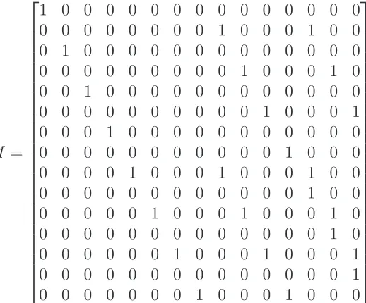
2. Clearly, Eqs. (18)-(21) are a consequence of the fact that in binary extension fields, squaring is a linear operation. The linear nature of binary extension field squaring, allow us to describe this operator in terms of an (m×m)-matrix as,
C =A2 =MA (22)
Furthermore, based on Eq. (22), it follows that computing the square root of an arbitrary field element A means finding a field element D = √A such that D2 =MD =A. Hence,
D=M−1A (23)
Eq. (23) is especially attractive for fields GF(2m) with order sufficiently large, i.e.,m >>2, where the matrixesMcorresponding to Eqs. (18)-(21) are all highly spare (each row has at most three nonzero values).
Hence, for the trinomial types I, II, III and IV as described above, the element D = √Agiven by Eq. (23) can be found by using the matrix form of Eqs. (18)-(21), respectively, followed by the computation of the inverse of the corresponding matrixM.
Using Eqs. (10) and (11), together with the fact thatM−1 = (N−1)T allow us to determine themcoordinates of the field element√a=d=M−1aas described bellow.
Type I: ComputingDsuch thatD2 =A modP(x), withP(x) =xm+xn+ 1, meven,nodd, andn < m
2:
di =
a2i+a2i+n i≤ bn2c, a2i+a(2i+n) modm+a2i−n bn2c< i < n, a2i+a(2i+n) modm n ≤i < m2, a(2i+n) modm m2 ≤i < m
(24)
fori = 0,1,· · · , m−1. It can be verified that Eq. (24) has an associated cost of m+n−1
2 XOR gates and2Tx delays.
Type II: ComputingDsuch thatD2 =A modP(x), withP(x) =xm+xn+ 1, meven,nodd andn= m
2:
di =
a2i+a2i+m2 i < m+24 , a2i m+24 ≤i < m2 a(2i+m2) modm m2 ≤i < m
(25)
fori = 0,1,· · · , m−1. It can be verified that Eq. (25) has an associated cost of m+2
Type III: ComputingDsuch thatD2 =AmodP(x), withP(x) =xm+xn+ 1, m,nodd numbers andn < m+1
2 ,
di =
a2i i < n+12 ,
a2i +a2i−n n+12 ≤i < m+12 , a2i−n+a2i−m m+12 ≤i < m+n2 , a2i−m m+n2 ≤i < m
(26)
fori = 0,1,· · · , m−1. It can be verified that Eq. (26) has an associated cost of m−1
2 XOR gates and oneTx delay.
Type IV: ComputingDsuch thatD2 =AmodP(x), withP(x) = xm+xn+ 1, m, odd,neven anddm−1
4 e ≤n <b m−1
3 c.
di =
a2i +a2i+(m−n)+a2i+(m−2n)+a2i+(m−3n) i < 4n−(m2 −1), a2i +a2i+(m−n)+a2i+(m−2n)+a2i+(m−3n)
+a2i+(m−4n) 4n−(m2 −1) ≤i < n2, a2i +a2i+(m−2n)+a2i+(m−3n)+a2i+(m−4n) n2 ≤i < 5n−(m2 −1), a2i +a2i+(m−2n)+a2i+(m−3n)+a2i+(m−4n)
+a2i+(m−5n) 5n−(m2 −1) ≤i < n,
a2i n≤i≤ m−21,
a2i−m m+12 ≤i < n+m+12 , a2i−m+a2i−(m+n) n+m+12 ≤i < 2n+m+12 a2i−m+a2i−(m+n)+a2i−(m+2n) 2n+m+12 ≤i < 3n+m+12 a2i−m+a2i−(m+n)+a2i−(m+2n)+a2i−(m+3n) 3n+m+12 ≤i < m
(27) fori= 0,1,· · · , m−1. At first glance, Eq. (27) can be implemented with an XOR gate cost of,
3·4n−(m−1)
2 + 4·
m−3n−1 2 + 3·
4n−(m−1)
2 +
4· m−3n−1
2 +
n 2 + 2·
n 2 + 3·
m−3n−1
2 = 5·
m−n−1
2 −
n 2. However, taking advantage of the high redundancy of the terms involved in Eq. (27), it can be shown (after a tedious long derivation) that actually
m+n−1
Table 1: Summary of complexity results
Type TrinomialP(x) =xm+xn+ 1 Operation XOR gates Time delay
I meven,nodd Squaring (m+n−1)/2 2Tx
II meven,n=m/2 Squaring (m+ 2)/4 Tx
III modd,nodd Squaring (m−1)/2 2Tx
IV modd,neven Squaring (m+n−1)/2 Tx
I meven,nodd Square root (m+n−1)/2 2Tx
II meven,n=m/2 Square root (m+ 2)/4 Tx
III modd,nodd Square root (m−1)/2 Tx
IV modd,neven Square root (m+n−1)/2 2Tx
Table 2: Irreducible trinomialsP(x) =xm+xn+ 1of degreem ∈[160,571]encoded
asm(n), withma prime number
m(n) Type m(n) Type m(n) Type 167(35) III 281(93) III 439(49) III
191(9) III 313(79) III 449(167) III 193(15) III 337(55) III 457(61) III 199(67) III 353(69) III 463(93) III 223(33) III 359(117) III 479(105) III 233(74) IV 367(21) III 487(127) III 239(81) III 383(135) III 503(3) III 241(70) IV 401(152) IV 521(158) IV 257(41) III 409(87) III 569(77) III 263(93) III 431(120) IV
Table 1summarizes the area and time complexities just derived for the cases considered. Furthermore, in Table 2 we list all preferred irreducible trinomials P(x) =xm+xn+ 1of degreem∈[160,571]withma prime number. In all the instances considered the computational complexity of computing the square root operator is comparable or better than that of the field squaring.
5 Illustrative Examples
In order to illustrate the approach just outlined, we include in this Section sev-eral examples using first the artificially small finite fieldGF(215) and then more realistic fields, in terms of practical cryptographic applications.
Table 3: Squaring matrixM of Eq. (22)
M =
1 0 0 0 0 0 0 0 0 0 0 0 0 0 0 0 0 0 0 0 0 0 0 1 0 0 0 1 0 0 0 1 0 0 0 0 0 0 0 0 0 0 0 0 0 0 0 0 0 0 0 0 0 0 1 0 0 0 1 0 0 0 1 0 0 0 0 0 0 0 0 0 0 0 0 0 0 0 0 0 0 0 0 0 0 1 0 0 0 1 0 0 0 1 0 0 0 0 0 0 0 0 0 0 0 0 0 0 0 0 0 0 0 0 0 0 1 0 0 0 0 0 0 0 1 0 0 0 1 0 0 0 1 0 0 0 0 0 0 0 0 0 0 0 0 0 0 1 0 0 0 0 0 0 0 1 0 0 0 1 0 0 0 1 0 0 0 0 0 0 0 0 0 0 0 0 0 0 1 0 0 0 0 0 0 0 1 0 0 0 1 0 0 0 1 0 0 0 0 0 0 0 0 0 0 0 0 0 0 1 0 0 0 0 0 0 0 1 0 0 0 1 0 0 0
Example 5.1. Field Square Root Computation overGF(215)
Table 4: Square root matrixM−1of Eq. (23)
M−1 =
1 0 0 0 0 0 0 0 0 0 0 0 0 0 0 0 0 1 0 0 0 0 0 0 0 0 0 0 0 0 0 0 0 0 1 0 0 0 0 0 0 0 0 0 0 0 0 0 0 0 0 1 0 0 0 0 0 0 0 0 0 1 0 0 0 0 0 0 1 0 0 0 0 0 0 0 0 0 1 0 0 0 0 0 0 1 0 0 0 0 0 0 0 0 0 1 0 0 0 0 0 0 1 0 0 0 0 0 0 0 0 0 1 0 0 0 0 0 0 1 0 1 0 0 0 0 0 0 0 1 0 0 0 0 0 0 0 0 1 0 0 0 0 0 0 0 1 0 0 0 0 0 0 0 0 1 0 0 0 0 0 0 0 1 0 0 0 0 0 0 0 0 1 0 0 0 0 0 0 0 0 0 0 0 0 0 0 0 0 1 0 0 0 0 0 0 0 0 0 0 0 0 0 0 0 0 1 0 0 0 0 0 0 0 0 0 0 0 0 0 0 0 0 1 0
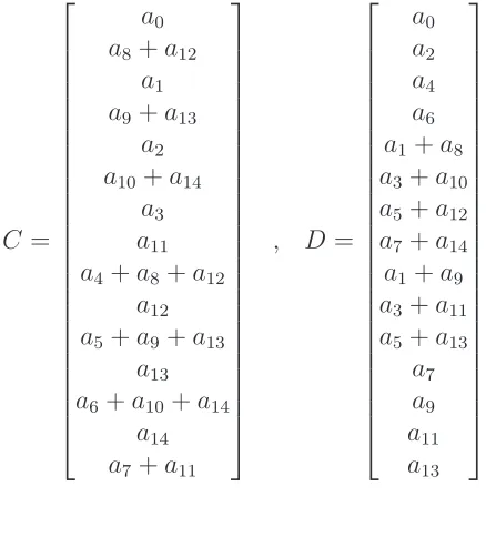
Table 5: Square and square root coefficient vectors.
C = a0
a8+a12
a1
a9+a13
a2
a10+a14
a3
a11
a4+a8+a12
a12
a5+a9+a13
a13
a6+a10+a14
a14
a7+a11
, D=
a0 a2 a4 a6
a1+a8
a3+a10
a5+a12
a7+a14
a1+a9
a3+a11
a5+a13
shown in Table3. Then, the inverse matrix ofM modulus two,M−1, is obtained as shown in Table 4. Afterwards, the polynomial coefficients, in terms of the co-efficients ofA, corresponding to the field squareC =A2and the field square root D=√Aelements can be found from Eqs. (22) and (23) as shown in Table5.
As predicted by Eq. (20), field squaring can be computed at a cost of(m−
1)/2 = (15−1)/2 = 7XOR gates and oneTxdelay. In the same way, the square root operation can be computed at a cost of (m2−1) = (152−1) = 7 XOR gates with an incurred delay time of oneTx, which matches Eq. (26) prediction. It is noticed that in this binary extension field, computing a field square root requires the same computational effort than the one associated to field squaring.
Example 5.2. Field Square Root Computation over GF(2162)
Let us consider GF(2162) generated using the irreducible Type II trinomial, P(x) = x162+x81+ 1. Using the same approach as for the precedent example, we can obtain the square root polynomial coefficients of an arbitrary element A from the fieldGF(2162)as,
di =
a2i+a2i+81 i <41, a2i 41≤i <81 a(2i+81) mod 162 81≤i
(28)
for i = 0,1,· · · ,161. As predicted by Eq. (25) the associated cost of the field square root computation for this field is given as, (m+2)4 = (162+2)4 = 41 XOR gates with an incurred delay time of oneTx.
Example 5.3. Field Square Root Computation over GF(2409)
Let GF(2409) be a field generated with the Type III irreducible trinomial, P(x) = x409 +x87 + 1 3. The square root of any arbitrary field element A is
given as,
di =
a2i i <44,
a2i+a2i−87 44≤i <205, a2i−87+a2i−409 205 ≤i <248, a2i−409 248 ≤i
(29)
3This is a NIST recommended finite field for elliptic curve applications [13]. It was used as an
for i = 0,1,· · · ,408. Eq. (29) can be implemented with an XOR gate cost of m−1
2 = 204 XOR gates with a 2Tx gate delay, which agrees with the value pre-dicted by Eq. (26).
Example 5.4. Field Square Root Computation over GF(2233)
Let GF(2233) be a field generated with the Type III irreducible trinomial, P(x) = x233 +x74 + 1 4. The square root of any arbitrary field element A is
given as,
di =
a2i+a2i+159+a2i+85+a2i+11 i <32, a2i+a2i+159+a2i+85+a2i+11+a2i−63 32≤i <37, a2i+a2i+85+a2i+11+a2i−63 37≤i <69, a2i+a2i+85+a2i+11+a2i−63+a2i−137 69≤i <74,
a2i 74≤i≤116,
a2i−233 116 ≤i <154, a2i−233+a2i−307 154 ≤i <191 a2i−233+a2i−307+a2i−381 191 ≤i <228 a2i−233+a2i−307+a2i−381+a2i−455 228 ≤i <233
(30)
for i = 0,1,· · · ,232. Eq. (30) can be implemented with an XOR gate cost of m+n−1
2 = 153 XOR gates with a 4Tx gate delay, which agrees with the value predicted by Eq. (27).
6 Applications
The square root operation has several relevant applications in the domain of ellip-tic curve cryptography, parellip-ticularly as an important building block for implement-ing the so-calledpoint halvingprimitive [14,15,3].
In the rest of this Section we describe how the square root operator can be applied for speeding up the computation of the exponentiation in binary extension fields.
4This is a NIST recommended finite field for elliptic curve applications [13]. It was used as an
6.1 Exponentiation over binary finite fields
Exponentiation over binary finite fields is used for inverse computation via Fer-mat Little theorem [7] and key agreement schemes such as the Diffie-Hellman protocol, among other applications.
For binary extension fieldsGF(2m), generated using them-degree irreducible polynomial P(x), irreducible over GF(2). Let e be an arbitrary m-bit positive integere, with a binary expansion representation given as,
e = (1em−2. . . e1e0)2 = 2m−1+ mX−2
i=0 2ie
i.
Then,
b =ae = a2m−1+Pmi=0−22iei (31)
= a2m−1
·a2m−2e
m−2 · · · · ·a21e1 ·a20e0 =a2m−1 ·
mY−2 i=0
a2ie i
Algorithm 1MSB-first binary exponentiation.
Require: The irreducible polynomialP(x),a∈GF(2m),e= (e
m−1. . . e1e0)2
Ensure: b=ae modP(x) 1: b=a;
2: fori=m−2downto0do
3: b=b2 ;
4: ifei == 1then
5: b=b·amodP(x);
6: Returnb
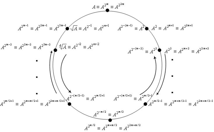
Figure 2: An illustration of the squaring and square root Abelian Groups (with A an arbitrary field element andman even number)
On the other hand, it is known from Fermat Little Theorem that for any nonzero a ∈ GF(2m), we havea2m−1
= 1 which implies a2m
= a and by taking square root in both sides of the last relation we geta2m−1
= √a =a2−1
. In general, the i-th square-root ofa, withi≥1can be written as,
a2m−i
=a2−i
.
In other words, the squaring and the square root operators form a multiplica-tive Abelian group of order m as is depicted in Fig.2. Considering an arbitrary elementA ∈ GF(2m), withmeven, Fig.2illustrates, in the clockwise direction, all themfield elements that can be generated by repeatedly computing squarings, i.e.,A2i
fori= 0,1,· · · , m−1. On the other hand, in the counterclockwise direc-tion, Fig.2illustrates all themfield elements that can be generated by repeatedly computing the square root operator, i.e.,A2−i
Hence, Eq. (31) can be reformulated in terms of the square root operator as,
ae = a2m−1
·
mY−2 i=0
a2ie
i =a2m−1 ·a2m−2em−2 · · · · ·a21e1 ·a20e0 (32)
= a2−1
·a2−2e
m−2 · · · · ·a2−(m−1)e1 ·a20e0 =√a·
mY−1 i=2
a2−ie i ·ae0
Algorithm 2Square root LSB-first binary exponentiation.
Require: The irreducible polynomialP(x),a∈GF(2m),e= (e
m−1. . . e1e0)2
Ensure: b=ae modP(x) 1: b=a;
2: em =e0;
3: fori= 1tomdo
4: b=√b;
5: ifei == 1then
6: b=b·amodP(x);
7: Returnb
Therefore, the novel square root LSB-first binary strategy requires a total of m−1square root computations andH(e)−1field multiplications, whereH(e) is the Hamming weight of the binary representation ofe. The pseudo-code of the square root LSB-first binary algorithm is shown in Algorithm2.
Algorithms 1 and 2 suggest a parallel version that can combine both ideas. This parallel version is especially attractive for hardware platforms implementa-tions. Algorithm 3shows this suggesting algorithm. Notice that both loop com-putations can be performed in parallel provided that the architecture has two inde-pendent field multiplier units. The computational time speedup can be estimated in about 50% when compared with Algorithms1and2.
7 Conclusion
Algorithm 3Squaring and Square root parallel exponentiation.
Require: The irreducible polynomialP(x),a∈GF(2m),e= (e
m−1. . . e1e0)2
Ensure: b=ae modP(x) 1: b=c=a;
2: em = 0; 3: N =bm
2c;
4: fori=N downto0do forj =N + 1tomdo
5: b=b2 ; c=√c;
6: ifei == 1then ifej == 1then
7: b=b·a; c=c·a;
8: b=b·c; 9: Returnb
exact cost of the square root operator, we categorized irreducible trinomials over
GF(2) into four different types. For all four types considered, explicit area and time complexity formulae were found for both, field squaring and field square root operators. It was shown that for the important practical case of finite fields generated using irreducible trinomials, the square root operation can be performed with no more computational cost than the one associated to the field squaring operation
It results instructive to also study the important practical case of finite fields generated by irreducible pentanomials. Unfortunately, our experiments show that the square root computation becomes much more expensive for this case. As a means of illustrating the pentanomial case, we applied the method described in Section4.2to the finite fieldGF(2163) generated with the irreducible pentanomial P(x) = x163+x7+x6+x3+ 1. The corresponding formulae for the square root computation of an arbitrary field elementA are shown in Appendix A. The total gate count is of about 1028 two-input XOR gates with a 6Txgate delays.
Field square root operator has several relevant applications in cryptography. In this contribution, we propose a novel application of the square root operator in the domain of exponentiation computation over binary extension fields. It was shown that by using as building blocks squarers, multipliers and square root blocks, a parallel version of the classical square-and-multiply exponentiation algorithm can be obtained. A hardware implementation of that parallel version may provide a speedup of up to 50% percent when compared with the traditional version.
curve cryptography.
ACKNOWLEDGMENTS
The authors are indebted to Darrel Hankerson and Alfred Menezes for suggestions of how to improve this paper.
References
[1] IEEE standards documents, IEEE P1363: Standard specifications for pub-lic key cryptography. Draft Version D18. IEEE, November 2004,
[2] J. Daemen and V. Rijmen, The design of Rijndael, AES-The Advance En-cryption Standard. Springer-Verlag Berlin-Heidelberg, New York, 2002. [3] D. Hankerson, A. Menezes, and S. Vanstone, Guide to Elliptic
Cryptogra-phy. Springer-Verlag, New York, 2004.
[4] R. Schroeppel, C. Beaver, R. Gonzales, R. Miller, and T. Draelos, “A low-power desing for an elliptic curve digital signature chip,” in Workshop on Cryptographic Hardware and Embedded Systems (CHES 2002), B. Kaliski, C. Koc, and C. Paar, Eds., vol. LNCS 2523. Springer-Verlag, August 2002, pp. 366–380.
[5] G. Orlando and C. Paar, “An efficient squaring architecture for GF(2m) and its applications in cryptographic systems,” IEE Electronic Letters, vol. 36, no. 13, pp. 1116–1117, June 2000.
[6] D. E. Knuth,The Art of Computer Programming 3rd. ed. Reading, Massa-chusetts: Addison-Wesley, 1997.
[8] K. Fong, D. Hankerson, J. L´opez, and A. Menezes, “Field inversion and point halving revisited.” IEEE Trans. Computers, vol. 53, no. 8, pp. 1047– 1059, 2004.
[9] R. Dahab, D. Hankerson, F. Hu, M. Long, J. Lopez, and A. Menezes, “Soft-ware multiplication using normal bases,” Dept. of Combinatorics and Op-timization, Univ. of Waterloo, Canada, Tech. Rep. Technical Report CACR 2004-12, 21 pages, 2004.
[10] A. Menezes, P. van Oorschot, and S. Vanstone,Handbook of Applied Cryp-tography. CRC Press, October 1996.
[11] H. Wu, “Low complexity bit-parallel finite field arithmetic using polynomial basis,” in Workshop on Cryptographic Hardware and Embedded Systems (CHES 99), ser. Lecture Notes in Computer Science, C. Koc and C. Paar, Eds., vol. 1717. Springer-Verlag, August 1999, pp. 280–291.
[12] ——, “On complexity of squaring using polynomial basis in GF(2m),” in
Workshop on Selected Areas in Cryptography (SAC 2000), S. T. D. Stinson, Ed., vol. LNCS 2012. Springer-Verlag, September 2000, pp. 118–129.
[13] National Institute of Standards and Technology (NIST), Recommended El-liptic Curves for Federal Government Use. NIST Special Publication, July
1999,
[14] R. Schroeppel, “Elliptic curve point ambiguity resolution apparatus and method,” International Application Number PCT/US00/31014, filed 9 No-vember 2000.
Appendix A: Field Square Root Computation over
GF
(
2
163)
LetGF(2163)be a field generated with the irreducible pentanomial,P(x) = x163+ x7+x6+x3+ 115. Given any arbitrary field elementA, themcoefficients of the
field elementD=√Acan be computed as shown in Table7.
d0 = P24j=0a159−6j⊕a9⊕a3⊕a0 d1 =
P26
j=0a6j+5⊕a2
d2 = P25j=0a6j+7⊕a4 d3 = a6⊕a3
d4 = a8⊕a5⊕a1
d5 = a10⊕a7⊕a3⊕a1 d6 =
P24
j=0a159−6j⊕a12⊕a5
d80 =
P26
j=0a6j+5⊕a160
P25
j=0a6j+3
d81 = P26j=0a6j+1⊕a162P25j=0a6j+5 d160 =
P26
j=0a6j+3
d161 = P26j=0a6j+5 d162 =
P26
j=0a6j+1
d3i+7 = P26j=0a6j+3⊕P24j=0−ia161−6j⊕a6i+14⊕Pij+1=0a6j+1, fori∈[0,24]
d3i+8 =
P26
j=0a6j+5⊕
P23−i
j=0 a6(i+j)+19⊕a6i+16⊕
Pi+1
j=0a6j+3, fori∈[0,23]
d3i+9 =
P26
j=0a6j+1⊕
P23−i
j=0 a6(i+j)+21⊕a6i+18⊕
Pi+1
j=0a6j+5,fori∈[0,23]
d3i+82 =
P26
j=0a6j+3⊕
P25−i
j=0 a157−6j, fori∈[0,25]
d3i+83 =
P26
j=0a6j+5⊕
P25−i
j=0 a159−6j, fori∈[0,25]
d3i+84 = P26j=0a6j+1⊕Pj25=0−ia161−6j, fori∈[0,25]
Table 6:m-coordinates of theGF(2163) field elementD=√A
We synthesized the equations shown in Table7using Xilinx ISE 8.1i design tool, targeting the FPGA virtex2v3000 device. The obtained area and Timing performance figures are shown below.
• The incurred area cost on xor’s gates is:
Total number of XOR gates : 524
1-bit xor7 : 1
1-bit xor9 : 1
1-bit xor12 : 2
1-bit xor4 : 57
1-bit xor5 : 15
1-bit xor6 : 67
1-bit xor3 : 45
1-bit xor2 : 336
![Table 2: Irreducible trinomials P( x ) =xm +xn + 1 of degree m ∈[ 160, 571] encodedas m( n ) , with m a prime number](https://thumb-us.123doks.com/thumbv2/123dok_us/1852393.1240443/14.595.110.532.182.323/table-irreducible-trinomials-p-degree-encodedas-prime-number.webp)