Generating Shorter Bases for Hard Random Lattices
Jo¨el Alwen∗ New York University
Chris Peikert†
Georgia Institute of Technology
May 24, 2010
Abstract
We revisit the problem of generating a ‘hard’ random lattice together with a basis of relatively short vectors. This problem has gained in importance lately due to new cryptographic schemes that use such a procedure to generate public/secret key pairs. In these applications, a shorter basis corresponds to milder underlying complexity assumptions and smaller key sizes.
The contributions of this work are twofold. First, we simplify and modularize an approach originally due to Ajtai (ICALP 1999). Second, we improve the construction and its analysis in several ways, most notably by making the output basis asymptotically as short as possible.
Keywords: Lattices, average-case hardness, cryptography, Hermite normal form
∗
Work performed while at SRI International.
†
1
Introduction
A (point) lattice is a discrete additive subgroup of Rm; alternatively, it is the set of all integer linear combinations of some linearly independentbasisvectorsb1, . . . ,bn ∈ Rm. Lattices appear to be a rich source of computational hardness, and in recent years,cryptographicschemes based on lattices have emerged as a promising alternative to more traditional ones based on, e.g., the factoring and discrete logarithm problems. Among other reasons, this is because lattice-based schemes have yet to be broken by efficient quantum algorithms (cf. [Sho97]), and their security can often be based merely onworst-casecomputational assumptions (rather thanaverage-caseassumptions, which are the norm in cryptography).
In 1996, Ajtai’s seminal work [Ajt96] in this area demonstrated a particular family of lattices for which, informally speaking, finding a short nonzero lattice vector in a randomly chosen lattice from the family is at least as hard as approximating some well-studied lattice problems in theworst case, i.e., foranylattice. This family of ‘hard random lattices’ has since been used as the foundation for several important cryptographic primitives, including one-way and collision-resistant hash functions, public-key encryption, digital signatures, and identity-based encryption (see, for example, [GGH96, MR04, Reg05, GPV08]).
Ajtai’s initial work also showed how to generate a hard random lattice together with knowledge of one relatively short nonzero lattice vector. The short vector can be useful as secret information in cryptographic applications; examples include an identification scheme [MV03] and public-key cryptosystems [Reg05, GPV08]. Shortly after Ajtai’s work, Goldreich, Goldwasser and Halevi [GGH97] proposed some public-key cryptographic schemes in which the secret key is an entireshort basisof a public lattice, i.e., a basis in which all of the vectors are relatively short in Euclidean length. Their method for generating a lattice along with a short basis was ad-hoc, and unfortunately does not produce lattices from the provably hard family defined in [Ajt96]. Although the algorithm and cryptosystem were later improved [Mic01] (following a practical cryptanalysis of the original scheme for real-world parameters [Ngu99]), there is still no known proof that the induced random lattices are actually hard on the average. Therefore, the schemes from [GGH97] lack worst-case security proofs. (We also mention that the digital signature scheme from [GGH97] has since been shown to be insecureregardlessof the particular method used for generating lattices [NR06].)
1.1 Our Contributions
Our first contribution is to elucidate and modularize Ajtai’s basic approach for generating a hard random lattice along with a relatively short basis. We endeavor to give a ‘top-down’ exposition of the key aspects of the problem and the techniques used to address them (in the process, we also correct some minor errors in the original paper).
One novelty in our approach is to base the algorithm and its analysis around the concept of theHermite normal form(HNF), which is an easily computable, unique canonical representation of an integer lattice. Micciancio [Mic01] has proposed using the HNF in cryptographic applications to specify a lattice in its ‘least revealing’ representation; here we use other nice properties of the HNF to bound the dimension of the output lattice and the quality of the resulting basis.
Our second contribution is to refine the algorithm and its analysis, improving it in several ways. Most importantly, we improve the length of its output basis fromm5/2 to the asymptotically optimalO(√m), wheremis the dimension of the output lattice (see Section 3 for precise statements of the new bounds). For the cryptographic schemes of, e.g., [GPV08], this immediately implies security under significantly milder worst-case assumptions: we need only that lattice problems are hard to approximate to within anO˜(n3/2)
factor, rather thanO˜(n7/2)as before.
We hasten to add that [GPV08, Section 5] briefly mentions that Ajtai’s algorithm can be improved to yield anO(m1+)bound on the basis length, but does not provide any further details. The focus of [GPV08] is on applications of a short basis, independent of the particular generation algorithm. The present work is a full exposition of an improved generation algorithm, and is meant to support and complement the schemes of [GPV08], and any other applications requiring a short basis.
1.2 Relation to Ajtai’s Construction
Our construction is inspired by Ajtai’s [Ajt99], but differs from it substantially in both the high-level structure and most of the details. The most significant similarity is a specially crafted unimodular matrix with small entries, which is used to ‘cancel out’ the necessarily large entries of another matrix that appears in the construction.
Departing from the approach of [Ajt99], our construction is guided from the ‘top down’ by two indepen-dent aspects of the construction: the block structure of the short output basis, and the probability distribution of the output lattice. This approach helps to illuminate the essential nature of the problem, and yields several technical simplifications. In particular, it lets us completely separate thestructural constraintson the output lattice from itsrandomization(by contrast, in [Ajt99] the structure and randomization are tightly coupled).
2
Preliminaries
For a positive integerk, let[k]denote the set{1, . . . , k};[0]is the empty set. We denote the set of integers modulo an integerq≥1byZq, and identify it with the set of integer residues{0, . . . , q−1}in the natural
way. The base-2logarithm is denotedlg.
Column vectors are named by lower-case bold letters (e.g.,x) and matrices by upper-case bold letters (e.g.,
X). Theith entry of a vectorxis denotedxi, and thejth column of a matrixXis denotedxj. We identify a
matrixXwith the ordered set{xj}of its column vectors, and definekXk= maxjkxjk. ForX ∈Rn×m andY ∈Rn×m0
having an equal number of rows,[X|Y]∈ Rn×(m+m0)
denotes the concatenation of the columns ofXfollowed by the columns ofY. Likewise, forX∈Rn×mandY ∈Rn
0×m
We leteidenote theith standard basis vector, where its dimension will be clear from context. Thed×d
identity matrix is denotedId; we omit its dimension when it is clear from context. We denote the (Euclidean)
unit sphere inRmbySm−1, i.e.,Sm−1 ={x∈Rm : kxk= 1}.
2.1 Matrix Decompositions
For an ordered setS={s1, . . . ,sm} ⊂Rmof linearly independent vectors, theGram-Schmidt orthogonal-izationSeofSis defined iteratively as follows:se1 =s1, and forj = 2, . . . , m,sej is the component ofsj orthogonal tospan(s1, . . . ,sj−1), i.e.,sej =sj−
P
i∈[j−1]sei· hsj,seii/hsei,seii.
For a matrix M ∈ Rm×n, a singular value decomposition is a factorization M = UΣV−1 where
U∈Rm×m,V∈
Rn×nare orthogonal square matrices andΣ∈Rm×nis diagonal with nonnegative entries. The diagonal entries ofΣcalled thesingular valuesofM, and are unique up to order. By definition, it follows that the largest (respectively, smallest) singular value ofMis the maximum (respectively, minimum) value ofkMxkover allx∈Sn−1. Note also that the singular values ofMandMtare the same.
2.2 Probability
For two probability distributionsD1, D2 (viewed as functions) over a finite setG, the statistical distance ∆(D1, D2)is defined to be 12Pg∈G|D1(g)−D2(g)|. It is easy to see that statistical distance is a metric;
in particular, it obeys the triangle inequality. We say that a distributionD (or a random variable having distributionD) is-uniform if its statistical distance from the uniform distribution overGis at most.
2.2.1 Hashing
LetX andYbe two finite domains. A familyHof functions mappingX toYis2-universalif for all distinct
x, x0 ∈ X,Prh←H[h(x) =h(x0)] = 1/|Y|.
Lemma 2.1(Simplified Leftover Hash Lemma [HILL99]). LetHbe a family of2-universal hash functions from a domainX to rangeY. Then forh← Handx← X chosen uniformly and independently,(h, h(x))is
1 2
p
|Y|/|X |-uniform overH × Y.
Let G be any finite, abelian, additive group, and let m ≥ 1 be an integer. For g ∈ Gm, define
hg:{0,1}m → Gashg(x) = Pi∈[m]xigi. The familyH = {hg}g∈Gm is2-universal: for any distinct
x,x0 ∈ {0,1}m, there exists somei∈ [m]such thatx
i−x0i = ±1; by conditioning on any fixed values
ofgj ∈ Gfor j 6= iand averaging over the choice ofgi, we have Prg←Gm[hg(x) = hg(x0)] = 1/|G|.
Therefore by Lemma 2.1, (g, hg(x))is 12
p
|G|/2m-uniform over the choice of uniformly random and
independentg←Gmandx← {0,1}m.
For various reasons, it will be important for us to work with balanced (mean zero), rather than binary (zero-one), random variables. Extendhgto have domain{−1,0,1}m, and let the entries ofxbe independent
and chosen to be0with probability 12, and1and −1 each with probability 14. Then(g, hg(x))is again
1 2
p
|G|/2m-uniform, becausexmay be seen as the difference between two independent uniformly random
variablesx0,x00← {0,1}m, andh
g(x) =hg(x0)−hg(x00). (Note that we choose not to work with Bernoulli
±1random variables, becauseH={hg}is not necessarily2-universal on the domain{±1}).
Finally, by the triangle inequality for statistical distance, we have that (hg, hg(x1), . . . , hg(xk)) is k
2
p
|G|/2m-uniform for independenth
2.2.2 Subgaussian Random Variables and Matrices
We say that a random variableXissubgaussianwithparameters >0(sometimes called thesubgaussian moment) if Pr[|X| > t] ≤ 2 exp(−t2/s2) for all t ≥ 0. In particular, any bounded random variable is subgaussian. The following is a standard fact about subgaussian random variables; see, e.g., [Ver07, Lecture 5] for a proof.
Fact 2.2. LetX1, . . . , Xkbe independent subgaussian random variables with parameterswith mean zero,
and letu∈Rkbe arbitrary. ThenPi∈[k]uiXiis subgaussian with parameters· kuk.
There is a well-developed theory for bounding the singular values of random matrices with independent entries (which need not be identically distributed). The following lemma is folklore in the area; see, e.g., [Ver07, Lecture 6] for a proof.
Lemma 2.3. LetX∈Rm×nbe a matrix whose entries are independent subgaussian random variables with parameters. There exists a universal constantC > 0such that the largest singular value ofXis at most
C·s·(√m+√n), except with probability2−Ω(m+n).
2.3 Lattices
Generally defined, alatticeΛis a discrete additive subgroup ofRm. In this work, we are concerned only with full-rank integerlattices, which are discrete additive subgroups ofZmhaving finite index, i.e., the quotient groupZm/Λis finite. The determinant ofΛ, denoteddet(Λ), is the cardinality|Zm/Λ|of this quotient group. Geometrically, the determinant is a measure of the ‘sparsity’ of the lattice.
A latticeΛ⊆Zmcan also be viewed as the set of all integer linear combinations ofmlinearly independent
basisvectorsB={b1, . . . ,bm} ⊂Zm:
Λ =L(B) =
Bc= X i∈[m]
cibi : c∈Zm
.
A lattice has infinitely many bases (whenm≥2), which are related to each other by unimodular transforma-tions, i.e.,BandB0 generate the same lattice if and only ifB=B0·Ufor some unimodularU∈Zm×m. The determinant of any basis matrixBcoincides with the determinant of the lattice it generates, up to sign:
|det(B)|= det(L(B)).
Every latticeΛ⊆Zmhas auniquecanonical basisH= HNF(Λ)∈Zm×mcalled itsHermite normal form(HNF). The matrixHis upper triangular and has non-negative entries (i.e.,hi,j ≥0with equality for
i > j), has strictly positive diagonals (i.e.,hi,i≥1for everyi), and every entry above the diagonal is strictly
smaller than the diagonal entry in its row (i.e.,hi,j < hi,ifori < j). Note that becauseHis upper triangular,
its determinant is simply the productQ
i∈[m]hi,i>0of the diagonal entries. For a lattice basisB, we write HNF(B)to denoteHNF(L(B)). Given an arbitrary basisB,H= HNF(B)can be computed in polynomial time (see [MW01] and references therein).
2.4 Hard Random Lattices
We will be especially concerned with a certain family of lattices inZmas defined by Ajtai [Ajt96]. A lattice from this family is most naturally specified not by a basis, but instead by aparity checkmatrixA∈Zn×m
for some positive integernand positive integer modulusq. (We discuss the parametersn,q, andmin detail below; see also the survey [MR09]). The lattice associated withAis defined as
Λ⊥(A) =
x∈Zm : Ax= X
j∈[m]
xj ·aj =0∈Znq
⊆Zm.
It is routine to check thatΛ⊥(A)contains the identity0∈Zmand is closed under negation and addition,
hence it is a subgroup of (and lattice in)Zm. Also observe thatΛ⊥(A)is ‘q-ary,’ that is,q·Zm ⊆Λ⊥(A) for everyA, so membership inΛ⊥(A)is determined solely by an integer vector’s entries moduloq.
2.4.1 Hermite Normal Form
LetH∈Zm×mbe the Hermite normal form of a latticeΛ = Λ⊥(A)for some arbitrary parity check matrix
A∈Zn×m
q . GivenA, the matrixHmay be computed efficiently (e.g., by first computing a basis ofΛ). In
one of our constructions, we use the fact that every diagonal entry ofHis at mostq, which we now prove. We can determineHas follows. Starting with the first columnh1 =h1,1·e1∈Λ, it must be the case that
A·h1 =h1,1·a1 =0∈Znq.
Letk≤qbe the smallest positive integer solution tok·a1 =0∈Znq. Thenk·e1 ∈Λ, so we must be able
to writek·e1 =Hzfor somez∈Zm. Now because every diagonalhi,i>0andHis upper triangular, it
must be the case thatzi = 0for alli >1. This implies thatz1·h1,1 =k, and because0< k≤h1,1, we
must havez1 = 1and thush1,1=k≤q.
More generally, suppose thath1, . . . ,hj−1 are determined for somej ∈[m]. Then by similar reasoning
as above,hj ∈Zmis given by the unique solution to the equation
hj,j·aj+
X
i∈[j−1]
hi,j·ai =0∈Znq
in whichhj,j >0is minimized and0≤hi,j < hi,i ≤qfor everyi < j. In particular,q·ejis a solution to
the above relation, hencehj,j≤q. We conclude by induction that every diagonal entry ofHis at mostq.
2.4.2 Geometric Facts
LetΛ = Λ⊥(A)for some arbitraryA∈Zqn×m. First, we havedet(Λ)≤qn, by the following argument: let φ: (Zm/Λ)→Znq be the homomorphism mapping the residue class(x+Λ)toAx∈Znq. Thenφis injective,
because ifφ(x+ Λ) =φ(x0+ Λ)for somex,x0 ∈Zm, we haveA(x−x0) =0which impliesx−x0 ∈Λ,
i.e.,x= x0 mod Λ. Therefore, there are at most|Zqn| =qn residue classes inZm/Λ. Minkowski’s first
inequality states that the minimum distance ofΛ(i.e., the length of a shortest nonzero lattice vector) is at
most √
m·det(Λ)1/m≤√m·qn/m. (2.1) For reasons related to Proposition 2.4 below, the family of lattices under discussion is most naturally parameterized byn(even thoughmis the lattice dimension), and the parametersq =q(n)andm=m(n)
are viewed as functions ofn. Givennandq=q(n), a typical choice of the parameterm, which essentially minimizes the bound in (2.1), ism=c·nlgqfor some constantc >0. Then by (2.1), the minimum distance ofΛ⊥(A)for anyA∈Zn×m
q is at most
√
For the above parameters, a simple counting argument shows that the above bound onλ1(Λ⊥(A))is
asymptotically tight, with high probability over the uniformly random choice ofA. For simplicity, suppose thatqis prime. (With a bit more care, the argument can be extended to compositeqas well.) Then for any fixed nonzeroz ∈ Zm, the probability over the choice ofAthatz ∈ Λ⊥(A), i.e., thatAz= 0 ∈
Znq, is
exactlyq−n. Then as long as
Nα,m:=
z∈Zm :kzk ≤√αm ≤qn/2
for some constantα > 0, a union bound implies thatλ1(Λ⊥(A)) ≥ √αm = Ω(√nlogq) except with probabilityq−n/2.
To boundNα,m, we use a result of Mazo and Odlyzko [MO90]. An immediate consequence of [MO90, Lemma 1] is that for any constantδ >1, there exists a constantα >0such thatNα,m≤δm. The desired bound holds by choosingδ=qn/2m= 21/2c>1. For larger choices ofm=c(n)·nlgqwherec(n) =ω(1), a more refined analysis using the Mazo-Odlyzko bound shows that the minimum distance remains bounded from below byΩ(pnlogq/logc(n)), and from above byO(√nlogq)because we can simply ignore the extra columns ofA.
2.4.3 Average-Case Hardness
The following proposition, proved first by Ajtai [Ajt96] (in a quantitatively weaker form) and in its current form in [MR04, GPV08], relates the average-case and worst-case complexity of certain lattice problems.
Proposition 2.4(Informal). For anym=m(n), β=β(n) = poly(n)and anyq =q(n)≥β·ω(√nlogn), finding a nonzerox ∈ Λ⊥(A)having length at mostβ for uniformly randomA ∈ Zn×m
q (with at least 1/poly(n)probability over the choice ofA and the randomness of the algorithm) is at least as hard as approximating several lattice problems onn-dimensional lattices to within aγ(n) =β·O˜(√n)factor in the worst case.
Note that Proposition 2.4 is meaningful only whenβis at least the typical minimum distance ofΛ⊥(A)
for uniformly randomA. Form=c·nlgqas described above, we can therefore takeβto be as small as
O(√nlgn), which yields a hard-on-average problem assuming the worst-case hardness of approximating lattice problems to within anO˜(n)factor.
In certain cryptographic applications, however, an adversary that breaks a cryptographic scheme is guaranteed only to produce a lattice vector whose length is substantially more than the minimum distance, so one needs average-case hardness for larger values ofβ. For example, the secret key in the digital signature schemes of [GPV08] is a basis ofΛ⊥(A)having some lengthL, and signatures are vectors of length≈L√m. It is shown that a signature forger may be used to find a nonzero lattice vector of lengthβ ≈L√minΛ⊥(A), which by Proposition 2.4 (for our choice ofm) is as hard as approximating lattice problems in the worst case to withinL·O˜(n)factors. Therefore, using a shorter secret basis in the signature scheme has the immediate advantage of a weaker underlying hardness assumption.
3
Constructions
We give two algorithms for constructing a hard random lattice together with a relatively short basis. Strictly speaking, our two constructions are incomparable. The first is relatively simple and gives a guaranteed bound on the basis quality, but is slightly suboptimal in either the lattice dimension or basis length. Our second construction is more involved, but it is simultaneously optimal (up to constant factors) in both the lattice dimension and another useful measure of quality.
Theorem 3.1. Letδ >0be any fixed constant. There is a probabilistic polynomial-time algorithm that, on input positive integersn(in unary),q, r≥2(in binary), andm≥(1 +δ)(1 +dlgrqe)·nlgq(in unary), outputs(A∈Zn×m
q ,S∈Zm×m)such that:
• Ais(m·q−δn/2)-uniform overZnq×m,
• Sis a basis ofΛ⊥(A), and
• kSk ≤2r√m.
Settingr = 2in the above theorem, the algorithm generates a basis of lengthO(√m) =O(pnlog2q)
for a random lattice having dimensionm=O(nlog2q). These quantities are larger than our ultimate goal byO(√logq)andO(logq)factors, respectively. Alternatively, ifq = poly(n), we may setr=nfor some small constant > 0, which implieslogrq =O(1). In this case, the algorithm generates a basis of only slightly suboptimal lengthO(n·√nlogq)for a random lattice having dimensionm=O(nlogq).
Our next constructionsimultaneouslyoptimizes the lattice dimension and basis quality, when the quality is measured according to theGram-Schmidt orthogonalizationof the basis. As explained in the introduction, this measure of quality is appropriate for all known applications. The somewhat large constant factor in the lower bound formis a consequence of the theorem’s generality, and can be improved in specific cases, such as whenqis a prime.
Theorem 3.2. Let δ > 0be any fixed constant. There is a probabilistic polynomial-time algorithm that, on input positive integersn(in unary),q ≥ 2(in binary), andm ≥ (5 + 3δ)·nlgq (in unary), outputs
(A∈Znq×m,S∈Zm×m)such that:
• Ais(m·q−δn/2)-uniform overZnq×m,
• kSk=O(nlogq)with probability1−2−Ω(n), and
• kSek=O(
√
nlogq)with probability1−2−Ω(n).
3.1 Common Approach
Here we describe the common framework, specified in Algorithm 1, that underlies the two concrete constructions from Theorems 3.1 and 3.2. (The details of each construction are given below in Sections 3.2 and 3.3, respectively.)
Letm=m1+m2for some sufficiently large dimensionsm1, m2. The algorithm is given a uniformly
random matrixA1 ∈Zqn×m1as input, and extendsA1toA= [A1|A2]∈Znq×mby generatingA2 ∈Znq×m2
Algorithm 1Framework for constructingA∈Zn×m
q and basisSofΛ⊥(A). Input: A1 ∈Znq×m1 and dimensionm2(in unary).
Output: A2∈Zqn×m2 and basisSofΛ⊥(A), whereA= [A1|A2]∈Zqn×mform=m1+m2.
1: Generate component matricesU∈Zm2×m2;G,R∈Zm1×m2;P∈Zm2×m1; andC∈Zm1×m1 such
thatUis nonsingular and(GP+C)⊂Λ⊥(A1), e.g., as described in Section 3.2 or 3.3. 2: LetA2 =−A1·(R+G)∈Znq×m2.
3: LetS=(G+UR)U RPP−C∈Zm×m.
4: return A2andS.
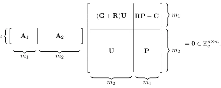
n A1 A2
| {z }
m1
| {z }
m2
(G+R)U RP−C
U P m1 m2
| {z }
m2
| {z }
m1
=0∈Znq×m.
The output matrixShas a block structure as shown in Figure 1, which uses four main component matrices
U,G,P, andRthat are provided by an instantiation of the framework. (The fifth matrixCis inessential to the basic construction, and is included only for some extra flexibility later on; for now we may takeC=0.) The components are named according to their essential properties:
• Uis nonsingular (invertible over the reals) and typically unimodular;
• Gtypically has entries that grow geometrically (from left to right);
• P‘picks out’ certain columns ofGvia the matrix productGP;
• Ris a random, typically ‘short’ matrix with an appropriate distribution (e.g., random0,±1entries). In both of our constructions, all of the components exceptRare constructed deterministically (depending on the inputA1), and the desired near-uniform distribution ofA= [A1|A2]follows from the uniformity ofA1
and the random choice ofR(via the leftover hash lemma). The utility ofS’s particular block structure will become clear as we see how it allows for satisfying the various constraints on the component matrices.
First, consider the requirement thatS⊂Λ⊥(A), i.e.,AS=0∈Zn×m
q . We need to satisfy
A1·(G+R)U+A2·U = 0∈Zn×m2
q (3.1)
A1·(RP−C) +A2·P = 0∈Znq×m1. (3.2)
We can immediately satisfy Equation (3.1) by letting
A2 =−A1·(G+R)∈Znq×m2. (3.3)
(Indeed, ifUis unimodular then this choice ofA2is necessary, becauseUcan be cancelled out of Equa-tion (3.1).) Note that for uniformly randomA1 and a suitable random choice ofR(independent of G),
the matrix [A1|A1R]will be close to uniformly random by the leftover hash lemma, hence so will the parity-check matrixA= [A1|A2] = [A1|−A1(G+R)].
Next, substituting Equation (3.3) into Equation (3.2) and rearranging, we obtain the constraint
A1·(GP+C) =0∈Znq×m1. (3.4)
That is, we need(GP+C) ⊂ Λ⊥(A1). Lemma 3.3 below shows that in order forSto be nonsingular, GP+Cmay be any basis or full-rank subset ofΛ⊥(A1). We will typically use the Hermite normal form
basisHNF(Λ⊥(A1)), due to its nice properties (specifically, efficient computability and bounded entries).
Lemma 3.3(Correctness of Algorithm 1). Adopt the notation and hypotheses of Algorithm 1. Then if
GP+C⊂Λ⊥(A1), we haveS⊂Λ⊥(A). Moreover,Sis a basis (respectively, full-rank subset) ofΛ⊥(A)
if and only ifGP+Cis a basis (resp., full-rank subset) ofΛ⊥(A1).
Proof. By the above discussion, we haveS⊂Λ⊥(A)ifGP+C⊂Λ⊥(A1). Now becauseUis unimodular, it is invertible. Using the formuladet W XY Z
=|det(X−WY−1Z)|(for square invertibleY) for the determinant of a block matrix, we have
|det(S)|=|det((RP−C)−(G+R)U·U−1·P)|=|det(GP+C)|.
by the columns ofA = [A1|A2], because the columns ofA2 =−A1(G+R)are inGby construction. Therefore,
det(Λ⊥(A)) =|G|= det(Λ⊥(A1)).
Thus|det(S)|= det(Λ⊥(A))— i.e.,Sis a basis ofΛ⊥(A)— exactly when|det(GP+C)|= det(Λ⊥(A1))
— i.e.,GP+Cis a basis ofΛ⊥(A1).
The remaining main constraint is thatSmust be relatively short. This presents a dilemma: clearlyP
must be short, but we need the columns ofGPto be nontrivial vectors inΛ⊥(A1), and it is hard to find short
nonzero vectors in this lattice. (Here we are assuming for simplicity thatC=0; in any case,Cneeds to be short becauseRis short as well.) Therefore, at least some of the columns ofGshould be ‘long.’ At the same time,GUmust be short because it appears inSas part of the block(G+R)U, and because bothUandR
are short.
The dilemma may be resolved by a judicious choice of theGandUmatrices. We constructGso that its columns grow geometrically to include long vectors that are themselves inΛ⊥(A1), or that have known small
combinations belonging toΛ⊥(A1). This makes it easy to construct a shortPso thatGP⊂Λ⊥(A1). We
also construct a short nonsingular matrixUso thatGUis short. This is possible because the small entries ofUcan cancel adjacent columns ofGto always yield short vectors. For example, the entries in thejth column ofGcan be2j, whileUcan simply have1s along the diagonal and−2s above the diagonal.
The remainder of the paper is dedicated to concrete instantiations of Algorithm 1, and to analyzing the quality ofSfor the particular constructions.
3.2 First Construction
We begin with a relatively simple instantiation of Algorithm 1. Its properties are summarized in the following lemma, of which Theorem 3.1 is an immediate corollary.
Lemma 3.4. Let δ > 0 be any fixed constant. There is a probabilistic polynomial-time algorithm that, given uniformly randomA1 ∈Zn×m1
q for anym1 ≥d= (1 +δ)nlgq, an integerr ≥2, and any integer m2 ≥m1·`(in unary) where`=dlogrqe, outputs matricesU,G,R,P, andC=Ias required by Step 1
of Algorithm 1 such that:
• A= [A1|A2]is(m2·q−δn/2)-uniform, whereA2is as in Step 2 of Algorithm 1.
• kSk ≤2r√m1+ 1, whereSis as in Step 3 of Algorithm 1.
The remainder of this subsection consists of the proof of Lemma 3.4.
3.2.1 Construction
GivenA1, letH∈Zm1×m1 be the Hermite normal form ofΛ⊥(A1). The basic idea of the construction is
thatGitself contains them1 columns ofH0 =H−I(among many others), andPsimply selects those
Definition ofG. Write
G=hG(1)|· · · |G(m1)|0i∈
Zm1×m2
as a block matrix consisting ofm1blocksG(i)having`columns each, and a final zero block consisting of
the remainingm2−m1·`columns (if any). As per our usual notation,gj(i)andh0j denote thejth columns
ofG(i) andH0, respectively. For eachi ∈ [m1],G(i) is defined as follows: let g(`i) = h0i, and for each j=`−1, . . . ,1, let
g(ji) =bgj(i+1) /rc=bh0i/r`−jc,
where the division and floor operations are coordinate-wise.
Note that because all the entries ofh0iare less thanq ≤r`, all the entries ofg1(i)are in the range[0, r−1].
Definition ofP. For eachj ∈[m1], letpj =ej` ∈ Zm2, the(j`)th standard basis vector. Observe that theith column ofPsimply selects the rightmost column ofG(i), yieldingGP=H0, as desired. Clearly,
kpjk2 = 1for allj∈[m1].
Definition ofU. Define the unimodular upper-triangular matrixT`∈Z`×`to have diagonal entries equal to1(i.e.,ti,i = 1for everyi∈[`]), upper diagonal entries equal to−r(i.e,ti,i+1 =−rfor everyi∈[`−1]),
and zero entries elsewhere. DefineU∈Zm2×m2 to be the block-diagonal matrix
U=diag(T`, . . . ,T`,I)
consisting ofm1blocksT`, followed by the square identity matrix of dimensionm2−m1·`.
Note thatUis unimodular and thatkujk2≤r2+ 1for allj. Also observe that
GU=
h
G(1)·T`|· · · |G(m1)·T`|0
i
.
We claim that all the entries of each block F(i) = G(i)·T` are integers in the range[0, r−1], and thus
kfj(i)k2 ≤m
1·(r−1)2. First observe that the claim is true forf1(i)=g (i)
1 , as explained above. Moreover,
for eachj∈[`−1]we have
fj(+1i) =gj(i+1) −r·gj(i)=g(ji+1) −r· bgj(i+1) /rc,
which establishes the claim.
Definition ofR. Each entry in the topd = (1 +δ)nlgq rows ofRis an independent{0,±1}-valued random variable that is0with probability 12,1with probability 14, and−1with probability14. The remaining entries are all0.
Observe thatkrjk2 ≤dfor allj. Also, by Lemma 2.1 and the discussion following it (withG=Znq), we
have thatA= [A1|−A1(G+R)]is(m2·q−δn/2)-uniform overZnq×m, as claimed. (Note that it is also
3.2.2 Quality ofS
We now analyze the length of the basis matrixS. By the triangle inequality and Pythagorean theorem,
kSk2 ≤max
(kGUk+kRUk)2+kUk2, kRP−Ik2+kPk2 .
We have
kPk2 = 1 and kRP−Ik2 ≤4d <4r2m 1,
because each entry ofRP−Ihas magnitude at most2. Therefore,kRP−Ik2+kPk2 <4r2(m 1+ 1).
Next, we have
kGUk2≤m1(r−1)2 and kRUk2≤d(r+ 1)2 ≤m1(r+ 1)2,
because every entry in the topdrows ofRUhas magnitude at mostr+ 1(and the other entries are zero). Thus(kGUk+kRUk)2 ≤4r2m1, and becausekUk2 ≤r2+ 1<4r2, the claim follows.
3.3 Second Construction
Theorem 3.2 is an immediate corollary of the following lemma.
Lemma 3.5. Let δ > 0 be any fixed constant. There is a universal constantC > 0and a probabilistic polynomial-time algorithm that, given uniformly randomA1 ∈Zn×m1
q for anym1≥d= (1 +δ)nlgq, and
any integerm2 ≥(4 + 2δ)nlgq(in unary), outputs matricesU,G,R,PandC=Ias required by Step 1
of Algorithm 1 such that:
• A= [A1|A2]is(m2·q−δn/2)-uniform, whereA2is as in Step 2 of Algorithm 1.
• kSk ≤Cnlgqwith probability1−2−Ω(n)over the choice ofR, whereSis as in Step 3 of Algorithm 1.
• kSek ≤1 +C
√
d=O(√nlogq)with probability1−2−Ω(n)over the choice ofR.
We have not attempted to optimize the exact constant Cappearing in the above bounds, but it is not exceedingly large (at most20, certainly). The remainder of this subsection is devoted to proving the lemma.
3.3.1 Construction
GivenA1, letH∈Zm1×m1 be the Hermite normal form ofΛ⊥(A1). The basic idea behind the construction is to ensure that the columns ofGinclude sufficiently many power-of-2multiples of each standard basis vectorei ∈ Zm1. This allows us to express each vector inH0 = H−Isimply as a binary combination of such vectors. (The−Iterm is included to make every entry in theith row ofH0 strictly smaller than
hi,i, which yields a tighter bound onm2.) To obtain a good bound on the length of the Gram-Schmidt
orthogonalizationeS, we additionally ensure that certain rows ofGare mutually orthogonal and sufficiently long. This ensures that adding the random matrixRtoGdoes not ‘distort the shape’ ofGby much, which is important in the analysis of the orthogonalization.
Recall that every diagonal entryhi,iof the Hermite normal formH∈Zm1×m1 is at least1, that Y
i∈[m1]
and that0≤hi,j < hi,ifor everyj 6=i. Therefore, every columnh0jofH0 =H−Ibelongs to the Cartesian
product
Y
i∈[m1]
[0, . . . , hi,i−1]⊂Zm1,
which has sizeQ
i∈[m1]hi,i≤q
n.
Definition ofG. Write
G=
h
G(1)|· · · |G(m1)|M|0
i
∈Zm1×m2
as a block matrix ofm1blocksG(i)having various widths, followed by a special blockM, followed by a
zero block of any remaining columns. For eachi∈[m1], blockG(i)has widthwi =dlghi,ie<1 + lghi,i,
and itsjth column isg(ji)= 2j−1·ei∈Zm1. Note that ifhi,i = 1, blockG(i)actually has width0, and that there are at mostnlgqvalues ofifor whichhi,i >1. Taking all blocksG(i)together, the total number of columns is therefore
X
i∈[m1]
wi ≤nlgq+
X
i∈[m1]
lghi,i ≤2nlgq.
(In the special case thatqis prime, there are at mostnvalues ofhi,ithat are greater than1, which are allq, so
the total number of columns in this case is at mostndlgqe.)
The blockMis a special component needed only for the analysis ofkeSk; the bound on the lengthkSk from Lemma 3.5 holds even if we leave outM(which allows for a smaller value ofm2). The blockMhas
widthw, wherewis the largest power of2in the range[d, m2−2nlgq]. Note thatm2−2nlgq≥2d, so a
power of2always exists in the given range, and thatw≥m2/2−nlgq≥m2/4.
Block Mis zero in all but its firstdrows, which are distinct rows of a square Hadamardmatrix of dimensionw, times a suitably large constantC0 >0. Recall that a Hadamard matrix is a square±1matrix whose rows are mutually orthogonal; a Hadamard matrix in any dimension2kmay be constructed in time
poly(2k)using Sylvester’s recursive formulaH2k =
H
2k−1 H2k−1
H2k−1 −H2k−1
, with base caseH1 = [1].
Definition ofP. Mirroring the structure ofG, we write
P=
h
P(1);· · ·;P(m1);0;0
i
∈Zm2×m1
as a vertical block matrix where each blockP(i)∈Zwi×m1.
For eachi, j∈[m1], thejth columnpj(i)ofP(i)contains the binary representation ofh0i,j ∈[0, . . . , hi,i−
1], which has length at mostwi. Specifically,P(i)contains entriesp(k,ji) ∈ {0,1}such that
h0i,j = X k∈[wi]
p(k,ji) ·2k−1.
Note thatkpjk2 ≤Pi∈[m1]wi≤2nlgq.
By definition ofG(i), we haveG(i)pj(i)=ei·Pk∈[m1]p
(i) k,j·2
k−1 =e
i·h0i,j, hence GP= X
i∈[m1]
G(i)P(i)=H0,
Definition ofU. LetTw ∈Zw×wbe the upper-triangular unimodular matrix with1s along the diagonal and−2s along the upper diagonal, i.e.,ti,i= 1fori∈[w]andti,i+1 =−2fori∈[w−1](all other entries
are zero). By definition ofG(i), observe thatF(i) =G(i)·Twi ∈Z
m1×wi is simplye
iin its first column
and zero elsewhere. Then lettingUbe the block diagonal matrix
U=diag(Tw1, . . . ,Twm1,I)∈Z
m2×m2,
we see thatUis unimodular and very short, i.e.,kUk2 ≤5, and that
GU=
h
F(1)|· · · |F(m1)|M|0
i
is also short, i.e.,kGUk ≤C0√d.
Definition ofR. Each entry in the topd = (1 +δ)nlgq rows ofRis an independent{0,±1}-valued random variable that is0with probability 12,1with probability 14, and−1with probability14. The remaining entries are all0.
Observe thatkrjk2 ≤dfor allj. Also, by Lemma 2.1 and the discussion following it (withG=Znq), we
have thatA= [A1|−A1(G+R)]is(m2·q−δn/2)-uniform overZnq×m, as claimed.
3.3.2 Quality ofS
We now analyzekSkandkSek. For both analyses, we partitionSinto two sets of vectors,
S1={sj}j∈[m2]= [(G+R)U;U] and S2 ={sj}j>m2 = [RP−I;P].
Length of basis vectors. We have
kSk= max{kS1k,kS2k}.
By the Pythagorean theorem and the triangle inequality,
kS1k2≤ kGU+RUk2+kUk2 ≤(C0
√
d+ 3
√
d)2+ 5≤(C
√
d+ 1)2, (3.5) for some large enough constantC >0.
ForkS2k, observe thatRis zero on all but ad×m2submatrix whose entries are independent subgaussian
random variables with some constant parameterC00>0. Therefore by Fact 2.2, for every fixedpj, the firstd
entries ofRpj ∈ Rm1 are independent subgaussian variables with parameterC00· kpjk = O(
√
nlogq). By Lemma 2.3, the largest singular value ofRpj, and hence the lengthkRpjk, is at mostO(
√
dnlogq) = O(nlogq)except with probability2−Ω(n). By the union bound and triangle inequality, we conclude that
kS2k=O(nlogq)except with probability2−Ω(n), as desired.
Length of Gram-Schmidt vectors. First we review some preliminary facts that are needed in the analysis. LetX∈Rm×`be any set of`≤mlinearly independent vectors. Thenπ
X:=X·(XtX)−1·Xt∈Rm×m is the projection matrix of the orthogonal linear projection fromRmtospan(X)⊆Rm. (Note that the Gram matrixXtXis invertible because the vectors inXare linearly independent.) This fact may be verified by observing that anyv∈span(X)may be written asv=Xcfor somec∈R`, hence
moreover, for anyv∈span⊥(X)we haveXtv=0and henceπX·v=0. Also note that for anyv∈Rm,
kπX·vk2 =hπX·v, πX·vi=hv, πX·vi=vt·πX·v= (Xtv)t·(XtX)−1·(Xtv), (3.6)
becausev−πX·vis orthogonal toπX·v.
In particular, we defineX∈Rm×m1 as
X= [−I|G+R]t,
and observe that the columns ofXare linearly independent and form a basis ofspan⊥(S1), because
dim span(X) =m1 =m−dim span(S1) and Xt·S1 =−(G+R)U+ (G+R)U=0.
We now analyzekSek. Observe that
kSek= max
j∈[m]
ksejk ≤max{kS1k,kπX·S2k}, (3.7)
becauseksejk ≤ ksjkfor allj ∈[m2], andsej is the orthogonal projection ofsj onto a linear subspace of
span(X)for allj > m2. Equation (3.5) has already established thatkS1k ≤C
√
d+ 1.
BoundingkπX·S2kis more involved. We start by setting up some additional notation that will make the
analysis more convenient. Define
ˆ
G= [−I|G], Rˆ = [0|R]∈Zm1×m, Pˆ = [0;P]∈
Zm×m1, S2ˆ =S2+ [I;0] = [R;I]·P. We have
kπX·S2k ≤ kπX·S2ˆ k+kπX·[I;0]k ≤ kπX·S2ˆ k+ 1,
by the triangle inequality and the fact thatπXrepresents an orthogonal projection onto a subspace ofRm. Therefore, it is enough to boundkπX·S2ˆ k. To do so, we analyze the two main components of the right-hand
side of Equation (3.6). We have
Xt·S2ˆ = [−I|G+R]·[R;I]·P=G·P= ˆG·Pˆ, XtX = ( ˆG+ ˆR)( ˆG+ ˆR)t.
We therefore want to analyze the properties of the positive semidefinite matrix
Z= ˆGt·( ˆG+ ˆR)( ˆG+ ˆR)t −1
·Gˆ. (3.8)
Note that the rows ofGˆ are orthogonal by construction (because the rows ofGare), that all its rows have length at least1, and that its firstdrows have length at leastC0√w ≥C0√m2/2by the properties of the
blockM. Therefore, we may factorGˆ as
ˆ
G=D·V
where the rows ofV∈Rm1×mare orthonormal (i.e.,VVt=I), andD∈Rm1×m1 is a nonsingular square
diagonal matrix whose firstddiagonal entries are all at leastC0√m2/2. BringingDinto the inverted central
term of Equation (3.8) from both sides, we therefore have
Below, we show that the singular values ofY =V+D−1Rˆ are all at least 12, with very high probability. Given this, it follows that the singular values ofZ, which are also its eigenvalues because Zis positive semidefinite, are all at most4. NowZmay be factored asZ=QΛQ−1for some orthogonal matrixQand diagonal matrixΛwhose diagonal entries are the eigenvalues ofZ. From this we have
kπX·S2ˆ k2 = max
j∈[m1]
kpˆtj ·Z·pˆjk2 ≤ max j∈[m1]
(4· kpˆjk2)≤8nlgq <(3
√
d)2.
It remains to bound the singular values ofY =V+D−1Rˆ from below by 12. To do so, it suffices to bound the singular values ofD−1Rˆ from above by 12, because by the triangle inequality and the fact that the rows ofVare orthonormal, the smallest singular value ofYis
min
x∈Sm−1kV
tx+ (D−1ˆ
R)txk ≥1− max
x∈Sm−1k(D
−1ˆ
R)txk ≥ 1
2.
By definition ofRˆ and the properties ofD, the matrixD−1Rˆ is zero on all but ad×m2submatrix whose
entries are independent subgaussian random variables of parameter1/(C00√m2), whereC00 >0is some
constant multiple ofC0. Lemma 2.3 implies that with probability1−2−Ω(d), the singular values ofD−1Rˆ
are all at most
C(√d+√m2) C00√m
2
≤ 1
2
(for sufficiently large constantC00), and the proof is complete.
Acknowledgments
We thank Daniele Micciancio and the anonymous referees for helpful comments on the presentation.
References
[Ajt96] M. Ajtai. Generating hard instances of lattice problems.Quaderni di Matematica, 13:1–32, 2004. Preliminary version in STOC 1996.
[Ajt99] M. Ajtai. Generating hard instances of the short basis problem. InICALP, pages 1–9. 1999.
[CHKP10] D. Cash, D. Hofheinz, E. Kiltz, and C. Peikert. Bonsai trees, or how to delegate a lattice basis. In EUROCRYPT. 2010. To appear.
[GGH96] O. Goldreich, S. Goldwasser, and S. Halevi. Collision-free hashing from lattice problems. Electronic Colloquium on Computational Complexity (ECCC), 3(42), 1996.
[GGH97] O. Goldreich, S. Goldwasser, and S. Halevi. Public-key cryptosystems from lattice reduction problems. InCRYPTO, pages 112–131. 1997.
[GHV10] C. Gentry, S. Halevi, and V. Vaikuntanathan. A simple BGN-type cryptosystem from LWE. In EUROCRYPT. 2010. To appear.
[HILL99] J. H˚astad, R. Impagliazzo, L. A. Levin, and M. Luby. A pseudorandom generator from any one-way function. SIAM J. Comput., 28(4):1364–1396, 1999.
[Mic01] D. Micciancio. Improving lattice based cryptosystems using the Hermite normal form. InCaLC, pages 126–145. 2001.
[MO90] J. E. Mazo and A. M. Odlyzko. Lattice points in high-dimensional spheres. Monatshefte f¨ur Mathematik, 110(1):47–61, March 1990.
[MR04] D. Micciancio and O. Regev. Worst-case to average-case reductions based on Gaussian measures. SIAM J. Comput., 37(1):267–302, 2007. Preliminary version in FOCS 2004.
[MR09] D. Micciancio and O. Regev. Lattice-based cryptography. InPost Quantum Cryptography, pages 147–191. Springer, February 2009.
[MV03] D. Micciancio and S. P. Vadhan. Statistical zero-knowledge proofs with efficient provers: Lattice problems and more. InCRYPTO, pages 282–298. 2003.
[MW01] D. Micciancio and B. Warinschi. A linear space algorithm for computing the Hermite normal form. InISSAC, pages 231–236. 2001.
[Ngu99] P. Q. Nguyen. Cryptanalysis of the Goldreich-Goldwasser-Halevi cryptosystem from Crypto ’97. InCRYPTO, pages 288–304. 1999.
[NR06] P. Q. Nguyen and O. Regev. Learning a parallelepiped: Cryptanalysis of GGH and NTRU signatures. J. Cryptology, 22(2):139–160, 2009. Preliminary version in Eurocrypt 2006.
[Pei09] C. Peikert. Public-key cryptosystems from the worst-case shortest vector problem. InSTOC, pages 333–342. 2009.
[PV08] C. Peikert and V. Vaikuntanathan. Noninteractive statistical zero-knowledge proofs for lattice problems. InCRYPTO, pages 536–553. 2008.
[PVW08] C. Peikert, V. Vaikuntanathan, and B. Waters. A framework for efficient and composable oblivious transfer. InCRYPTO, pages 554–571. 2008.
[Reg05] O. Regev. On lattices, learning with errors, random linear codes, and cryptography. J. ACM, 56(6), 2009. Preliminary version in STOC 2005.
[Sho97] P. W. Shor. Polynomial-time algorithms for prime factorization and discrete logarithms on a quantum computer. SIAM J. Comput., 26(5):1484–1509, 1997.