Uncertainty and Sensitivity Analysis of Dynamic Biological Systems under Data Sparseness.

(1)

ABSTRACT

BASNET, LOCHAN. Uncertainty and Sensitivity Analysis of Dynamic Biological Systems under Data Sparseness. (Under the direction of Joel J. Ducoste)

Systems biology integrates experimental observations with mathematical models to infer

the behavior of biological organisms at the genetic and metabolic levels. Ordinary

Differential Equation (ODE) based dynamic models are frequently used to describe these

biological behaviors under dynamic and steady state conditions. ODE-‐based models are

flexible in structure but may involve a large number of parameters. Under data sparseness

from the lack of experimental replicates under transient conditions, the parameters that are

estimated have uncertainties associated with them. Parameter uncertainties get

propagated through the model into the outputs resulting in misleading predictions and

inferences. A comprehensive understanding of these uncertainties can, however, prevent

such misleading deductions as well as provide valuable information about the behavior of

the biological systems. Given the scope of dynamic models in biological studies, such

comprehensive uncertainty studies for these models are lacking.

In this research, our aim was to perform a comprehensive uncertainty study of ODE-‐based

dynamic models under data sparseness. Through such study, our goal was to quantify the

uncertainty in the model parameters and outputs, assess the identifiability of these

(2)

output uncertainties under data sparseness. We studied two ODE-‐based dynamic models:

the yeast synthetic network model in Saccharomyces cerevisiae and a preliminary iron deficiency response model in Arabidopsis thaliana. In this research, an assessment of the accuracy of these methods was provided to deduce the biological information for both

systems. As part of this assessment, we demonstrated the applicability of the Morris

Screening method for sensitivity analysis of dynamic models. Through the bootstrap

method of uncertainty analysis, we calculated confidence intervals that encapsulated true

parameter values as well as the true expression of the genes in the yeast synthetic network

model. Assessment of practical identifiability using profile likelihood showed that the data

sparseness was high for both system models. Finally, the Morris Screening method was able

to identify the important and the unimportant parameters based on their contribution to

the output uncertainties for both of the models. Based on the results from Morris

Screening, we were able to explain the regulatory effects of SWI5 and ASH1 genes on CBF1

gene in the yeast synthetic network model. For the iron transcription factors in the

Arabidopsis thaliana gene regulatory network, we identified a clear influence of iron effect in the gene expression for COL4 and of constitutive transcription and degradation in the

gene expression of bHLH104, however, similar deductions could not be made for the

remaining transcription factors in the network. Sensitivity results identified the least

important parameters in the yeast synthetic network model that could be screened out for

the purpose of addressing data sparseness in any future analyses.

(3)

(4)

Uncertainty and Sensitivity Analysis of Dynamic Biological Systems under Data Sparseness

by Lochan Basnet

A thesis submitted to the Graduate Faculty of North Carolina State University

in partial fulfillment of the requirements for the Degree of

Master of Science

Civil Engineering

Raleigh, North Carolina

2017

APPROVED BY:

_________________________ _________________________

Cranos M. Williams, PhD Ranji Ranjithan, PhD

_________________________ Joel J. Ducoste, PhD

(5)

DEDICATION

To my sister Ritu Basnet,

Thank you for the support, love and guidance in every walk of my life.

To my mother and father,

Thank you for your love, care and all the opportunities you have provided that I feel blessed of.

(6)

BIOGRAPHY

Lochan Basnet was born in Pokhara, Nepal. He completed his undergraduate studies

as a Civil Engineer in year 2013 from Nepal. In the fall of 2015, he joined North Carolina

State University and began his pursuit of Master of Science in Civil Engineering under the

guidance of Dr. Ducoste.

(7)

ACKNOWLEDGEMENTS

I would first like to thank my advisor Dr. Joel J. Ducoste for providing me the opportunity to

be a part of such wonderful research. I am grateful for his continuous support,

encouragement, guidance, and valuable advice without which this thesis would not have

been possible. You are a great teacher and a wonderful person.

I also want to thank my thesis committee member and the principal investigator for the

research Dr. Cranos M. Williams for the critical analysis of my work and the valuable insights

that has helped me throughout my study. I am very grateful to the entire INSPIRE group for

providing me the data and the model used in this study.

I am thankful to Dr. Ranji Ranjithan for taking time to serve in my thesis committee. I am

also thankful to all the faculty and staff of the Department of Civil Engineering. Many thanks

to Renee Howard for all the timely information that helped me remain in right track

throughout the pursuit of my Master’s degree.

I would like to thank the National Science Foundation for the financial support.

(8)

TABLE OF CONTENTS

LIST OF TABLES ... vii

LIST OF FIGURES ... viii

SUPPLEMENTAL TABLES ... ix

SUPPLEMENTAL FIGURES ... x

CHAPTER 1 ... 1

Introduction ... 1

1.1 Objectives ... 3

CHAPTER 2 ... 5

Background ... 5

2.1 Dynamic system models and uncertainty ... 5

2.2 Uncertainty Analysis ... 5

2.2.1 Non-‐sampling based Uncertainty Analysis ... 7

2.2.2 Sampling based Uncertainty Analysis ... 8

2.3 Sensitivity Analysis ... 10

2.3.1 Local Sensitivity Analysis ... 11

2.3.2 Global Sensitivity Analysis ... 12

2.4 Preliminary Iron deficiency response model in Arabidopsis thaliana ... 14

CHAPTER 3 ... 16

Methods ... 16

3.1 Model ... 16

3.1.1 Yeast Synthetic Network Model in Saccharomyces cerevisiae ... 16

3.1.2 Preliminary Iron Deficiency Response Model in Arabidopsis thaliana ... 19

3.2 Bootstrap Sampling for Data Generation ... 19

3.3 Parameter Estimation ... 21

3.4 Uncertainty Analysis ... 21

3.5 Identifiability Analysis ... 22

3.6 Sensitivity Analysis ... 23

3.6.1 Extension to Morris Method ... 24

CHAPTER 4 ... 26

(9)

4.1 Introduction ... 27

4.2 Background ... 30

4.2.1 Dynamic system models and uncertainty ... 30

4.2.2 Uncertainty Analysis ... 30

4.2.3 Sensitivity Analysis ... 32

4.2.4 Iron deficiency response model in Arabidopsis thaliana ... 33

4.3 Methods ... 35

4.3.1 Model ... 35

4.3.2 Bootstrap Sampling for Data Generation ... 37

4.3.3 Parameter Estimation ... 39

4.3.4 Uncertainty Analysis ... 39

4.3.5 Identifiability Analysis ... 39

4.3.6 Morris Screening for Sensitivity Analysis ... 40

4.4 Results ... 42

4.4.1 Yeast Synthetic Model in Saccharomyces cerevisiae ... 42

4.4.2 Iron Deficiency Model in Arabidopsis thaliana ... 48

4.5 Discussion ... 55

4.6 Conclusion ... 58

CHAPTER 5 ... 59

Conclusion and Future Work ... 59

BIBLIOGRAPHY ... 62

APPENDIX ... 74

(10)

LIST OF TABLES

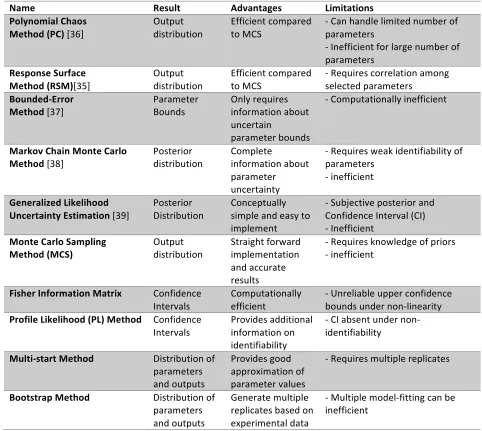
Table 2.1: Comparison of frequently used UA techniques ... 7

Table 2.3: Comparison of commonly used SA methods ... 11

Table 4.1: Parameters ranked by Savage scores under Fe-‐ condition ... 55

(11)

LIST OF FIGURES

Figure 1: Iron Deficiency Gene Regulatory Network in Arabidopsis thaliana: ... 15

Figure 2: Yeast Synthetic Network in Saccharomyces cerevisiae: ... 18

Figure 4.1: Iron Deficiency Gene Regulatory Network in Arabidopsis thaliana: ... 34

Figure 4.2: Yeast Synthetic Network in Saccharomyces cerevisiae: ... 36

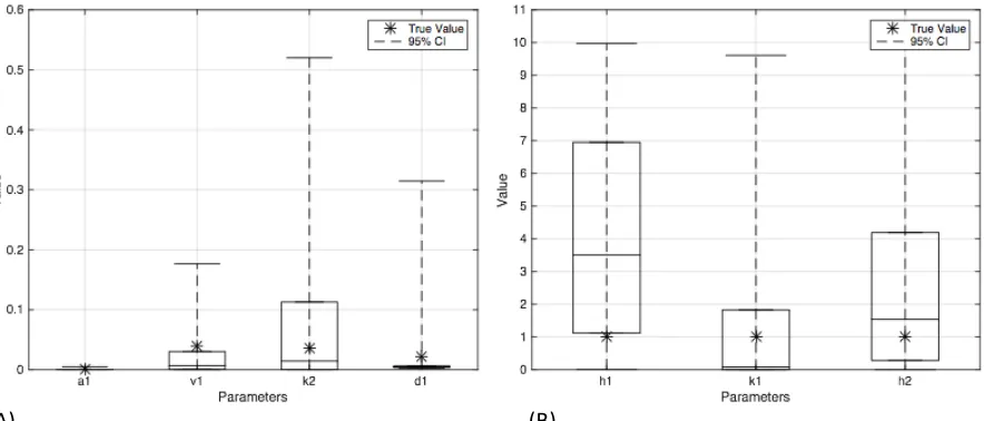
Figure 4.3 Boxplots of few parameters in Yeast synthetic model ... 43

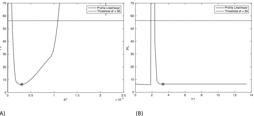
Figure 4.4: Profile Likelihood plots for assessing practical identifiability ... 45

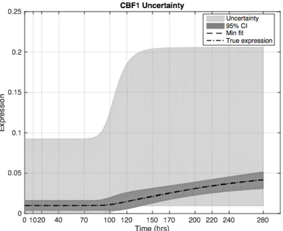
Figure 4.5: Output Uncertainty for CBF1 ... 46

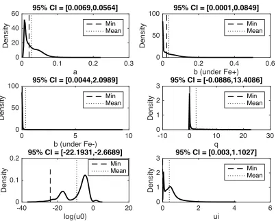
Figure 4.6: Parameter distributions for COL4 parameters: ... 50

Figure 4.7: Uncertainty for COL4 ... 52

(12)

SUPPLEMENTAL TABLES

Table S1: Comparison of frequently used UA techniques ... 122

Table S2: Comparison of commonly used SA methods ... 123

Table S3: Coefficient of Variation for the 30 parameters in the Yeast synthetic network

model in Saccharomyces cerevisiae ... 124 Table S4: Sensitivity rankings based on absolute mean elementary effects calculated by

Morris Screening and the overall rank based on the Savage scores for Yeast synthetic

network model in Saccharomyces cerevisiae ... 125 Table S5: Decay rates obtained from statistical analysis on the half-‐life experiment... 126

(13)

SUPPLEMENTAL FIGURES

Figure S1: Comparison of model Dynamics: ... 75

Figure S2: Bootstrap size selection ... 78

Figure S3: Boxplots for the 30 parameters of Yeast synthetic network model in

Saccharomyces cerevisiae ... 79

Figure S4: Uncertainty in the gene expression outputs for the 5 genes in Yeast synthetic

network model ... 83

Figure S5: Time varying sensitivity diagrams for GAL4 ... 87

Figure S6: Parameter uncertainties in the iron deficiency response model in Arabidopsis thaliana ... 88 Figure S7: Profile Likelihood plots for identifiability analysis ... 95

Figure S8: Total uncertainty in gene expressions under Fe-‐ for genes in iron deficiency

response model in Arabidopsis thaliana ... 114 Figure S9: 95% confidence intervals for gene expressions under Fe + (dark grey region) and

(14)

CHAPTER 1

Introduction

Systems Biology [1], [2] aims to understand the behavior of interacting biological system

components by gathering experimental observations and deciphering the implication of

these interactions with mathematical reasoning [3]. These observations and reasoning can

be used to understand and develop gene regulatory networks and perform metabolic

pathway analyses to explain how organisms function relative to environmental stresses or

under transgenic conditions [4]–[6].

At the genetic level, high-‐throughput experimental methods like microarray, qRT-‐PCR [7],

and RNA-‐SEQ [8], [9] are primarily employed to collect information required to develop a

gene regulatory network and to help build predictive mathematical relationships. However,

much of these experimental techniques are costly and sometimes time consuming to repeat

thus resulting in insufficient collection of data. This insufficient data poses a barrier for

researchers studying a biological system. The barrier is even greater when complex dynamic

mathematical models are used to identify and understand the interactions occurring in the

biological system.

Ordinary Differential Equations (ODEs), a type of mathematical model, are frequently

employed as dynamic models to track important inputs and their influence on transient

(15)

important to estimate to achieve the best model fit to the experimental data. The lack of

sufficient experimental data, however, leads to a condition of sparseness where the

number of model parameters exceeds the available experimental data. The parameter

values obtained under such sparse conditions can have uncertainties associated with them

that lead to inaccurate model outputs [4], [14]–[17]. If these uncertainties in parameters

are ignored, then erroneous conclusions can be inferred from the modeling results. The

need to understand and quantify the uncertainties related to mathematical models have led

to the introduction of uncertainty analysis and sensitivity analysis [18]–[20]. These

approaches have been extensively used in other areas such as risk analysis [21]–[23].

Several studies that make use of the uncertainty and sensitivity analyses in systems biology

have been reported [24]–[28]. However, these studies seem to be lacking one or more

points that might cause confusion among researchers looking to incorporate the

uncertainty and sensitivity analyses in their studies. These points include the following:

• The quantification of output uncertainty due to variability in parameters involves

two steps: parameter uncertainty quantification and forward propagation of

parameter uncertainty. Forward propagation refers to propagating the uncertainty

of the parameters by applying the uncertainty in the model equations. However, in

most of the systems biology studies, the parameter uncertainties are not calculated

(16)

differently under varied conditions, the assumed parameter uncertainties might not

be accurate thus resulting in an incorrect assessment of output uncertainties.

• A comprehensive understanding of uncertainty includes quantifying the variation in

the parameters and the outputs (i.e. uncertainty analysis/quantification),

determining the importance of parameters in relation to the change in output (i.e.

sensitivity analysis), and assessing if the parameters are identifiable (i.e.

identifiability analysis). These three analyses provide different information about

the model and the system under study. The information obtained is often

complementary and exclusive thus assisting in better understanding the model and

the system behavior under study. However, most system biology studies focus on

only one of these aspects of uncertainty that potentially results in an incomplete

understanding of the system.

• Sensitivity analysis for dynamic models include studies demonstrating the

application of variance-‐based methods [29], [30]. However, researchers have shown

that these methods are computationally intensive and infeasible for complex

systems. Screening methods, especially the method of Morris, is considered to be

an efficient alternative. However, the practical relevance of Morris Screening,

particularly to biological models, is somewhat unclear.

1.1 Objectives

(17)

• To affirm the need to conduct uncertainty analysis in the presence of data

sparseness;

• To perform the uncertainty analysis, the sensitivity analysis and the identifiability

analysis on a dynamical system model to illustrate a comprehensive understanding

of mathematical model uncertainty;

• To illustrate the use of Morris Screening in dynamic models; and

• To use the uncertainty information to develop a better understanding of iron effects

on gene expression of transcription factors in the Arabidopsis thaliana gene regulatory network

• To assess whether the parameter sensitivity analysis can be used to decrease the

sparseness in a dynamical biosystem model.

A successful completion of these analyses will provide great insight into the model behavior

and the model parameters. This information in turn will help decipher the different

biological interactions and properties of the biosystems under study.

(18)

CHAPTER 2

Background

2.1 Dynamic system models and uncertainty

There are a significant number of different models for biological systems. Broadly, these

models are classified under two types: static models and dynamic models. Although a

successful history of static models have been applied to systems biology studies [31], [32],

the use of dynamic models has a greater potential for success. The reason for greater

success is that a dynamic model can provide the systems behavior over time, unlike static

models that provide information only at a particular state [33]. However, dynamic models

are limited and typically include a large number of parameters that need to be estimated

with sparse data. Under such sparse conditions, large uncertainties are associated with the

parameters as well as the predictions. These uncertainties could lead to incorrect inferences

about the system. To ensure better understanding of the system, the uncertainties in the

dynamic models must be understood properly. However, studies that perform a

comprehensive assessment of uncertainties in dynamic models are lacking.

2.2 Uncertainty Analysis

Parameter uncertainty analysis is important in the evaluation of any mathematical model

and critically important when these models are evaluated with sparse data sets. Uncertainty

Analysis (UA) consists of two components: parameter uncertainty quantification and

(19)

the uncertainty would be to initially assess the parameter uncertainty and then propagate

this uncertainty into the model to determine the model output uncertainty. Yet, most of the

uncertainty analysis performed in systems biology have only utilized forward propagation

based on some form of random sampling [35]. The parameter uncertainty in these studies is

either based on a priori knowledge or is assumed. Such assessments are not accurate

because system behavior and properties vary for different conditions. Several uncertainty

analysis methods frequently used in systems biology studies as well as in other disciplines

are listed in Table 2.1. The table summarizes the type of results obtained, the advantages

and the limitations of the uncertainty analysis methods. In the sections following, these

methods are discussed based on the findings from previous studies. Moreover, the

advantages and applicability of one of the uncertainty analysis methods, Bootstrap method

used in this study, is highlighted.

(20)

Table 2.1: Comparison of frequently used UA techniques

Name Result Advantages Limitations

Polynomial Chaos

Method (PC) [36] Output distribution Efficient compared to MCS -‐ Can handle limited number of parameters -‐ Inefficient for large number of parameters

Response Surface

Method (RSM)[35] Output distribution Efficient compared to MCS -‐ Requires correlation among selected parameters

Bounded-‐Error

Method [37] Parameter Bounds Only requires information about uncertain

parameter bounds

-‐ Computationally inefficient

Markov Chain Monte Carlo

Method [38] Posterior distribution Complete information about parameter uncertainty

-‐ Requires weak identifiability of parameters

-‐ inefficient

Generalized Likelihood

Uncertainty Estimation [39] Posterior Distribution Conceptually simple and easy to implement

-‐ Subjective posterior and Confidence Interval (CI) -‐ Inefficient

Monte Carlo Sampling

Method (MCS) Output distribution Straight forward implementation and accurate results

-‐ Requires knowledge of priors -‐ inefficient

Fisher Information Matrix Confidence Intervals

Computationally efficient

-‐ Unreliable upper confidence bounds under non-‐linearity

Profile Likelihood (PL) Method Confidence Intervals

Provides additional information on identifiability

-‐ CI absent under non-‐ identifiability

Multi-‐start Method Distribution of parameters and outputs

Provides good approximation of parameter values

-‐ Requires multiple replicates

Bootstrap Method Distribution of parameters and outputs

Generate multiple replicates based on experimental data

-‐ Multiple model-‐fitting can be inefficient

2.2.1 Non-‐sampling based Uncertainty Analysis

Polynomial Chaos (PC) method and Response Surface Method (RSM) [35] are two popular

non-‐sampling based methods. PC, based on the concept of Wiener [36], uses spectral

(21)

on applying and improving PC methods. These studies show that PC methods are efficient

compared to Monte-‐Carlo methods, yet in the presence of large number of uncertainties,

these methods become inefficient. Debusschere et al. [47] discuss the numerical challenges

of applying PC methods and showed that high PC orders are necessary to avoid negative

values for strictly non-‐negative parameters and truncation errors at a high computational

cost. RSM [35] develops a response surface using few selected parameters to describe the

relationship between parameters and output. RSMs work better when they are highly

correlated but may not be able to detect important interactions when two parameters are

super-‐additive [48]. Both, PC and RSM are forward propagating uncertainty methods.

Another, non-‐sampling based method is the bound-‐error method [37]. Bound-‐error method

is based on interval analysis method which does not require probability distribution

information of the uncertain parameters. It rather assumes the bounds of the parameters

to quantify uncertainty. Several works have used this method and improvements have been

put forward [49]–[51]. Yet, the interval analysis based bound-‐error methods can still be

computationally infeasible for complex biological models.

2.2.2 Sampling based Uncertainty Analysis

Sampling based uncertainty analysis falls under two approaches: Bayesian approach and

Frequentist approach. Bayesian methods are probabilistic approaches based on Bayesian

theory while the frequentist approaches are based on multiple model fitting [52]. Most

(22)

(GLUE) of Beven and Binley [39] and Markov Chain Monte Carlo (MCMC) [38] methods.

GLUE and MCMC result in posterior probability that expresses the parameter uncertainty.

However, the posteriors obtained from GLUE are subjective and may not be the true

parameter uncertainty distribution. Like all Bayesian methods, both GLUE and MCMC

require the knowledge of priors [53]. Vrugt et al. [54] compared GLUE, and two MCMC

based approaches, Diﬀerential Evolution Adaptive Metropolis (DREAM) [55] and Delayed

Rejection Adaptive Metropolis (DRAM) [56].They observed that GLUE resulted in similar

estimates of parameter and prediction uncertainty as MCMC approaches. However, MCMC

based DREAM was much more efficient with regards to number of model evaluations

compared to GLUE and DRAM. According to Iorgulescu et al. [57], GLUE may require billions

of model evaluations to generate only a few good solutions. Though, DREAM MCMC is

efficient in comparison with GLUE and DRAM, it can still be inefficient and infeasible for

complex and stiff biosystem models [58]. Yang et al. [48] pointed out the difficulty in

constructing a likelihood function and the difficulty in assessing multi-‐modal distributions

with MCMC approaches.

Methods that fall under the frequentist approach are the Fisher Information Matrix (FIM),

the Profile Likelihood method (PL), the Multi-‐start method and the Bootstrapping method.

These methods result in the confidence intervals (CIs)of the parameters. Multi-‐start and the

bootstrap result in parameter distributions [59]–[62]. Studies have shown that the

(23)

parameters are identifiable [63], [64]. However, Joshi et al. [62] showed that FIM has two

important shortcomings: 1) it only provides lower bounds when the model is non-‐linear and

2) the confidence interval is symmetric which may not be true in all models. In addition, FIM

is a parameter dependent measure and requires prior knowledge about the parameters

[65].

The PL approach provides information about identifiability of parameters [16], [66], [67].

Multi-‐start methods can be used along with bootstrap methods to quantify parameter

uncertainties. Bootstrap methods are able to generate multiple samples based on few

experimental observations. These samples are used to quantify the parameter uncertainties

and subsequently the output uncertainties thus making them suitable for systems biology

studies. However, multiple model fitting of bootstrap samples can be computationally

expensive for complex models.

2.3 Sensitivity Analysis

Sensitivity Analysis (SA) quantifies the impact of parameter uncertainties on the model

outputs [68]. The objective of SA is to identify critical inputs (parameters and initial

conditions) of a model. Some of the important and frequently used SA methods are

compared in Table 2.3. The review below reports the findings of several SA studies to

establish the appropriate SA method for dynamic systems.

(24)

Table 2.3: Comparison of commonly used SA methods

Name Type Advantages Disadvantages

1. Local SA Local -‐ Easy

implementation -‐ Low computational cost

-‐ Non-‐generalizable results

-‐ Unable to detect parameter interactions 2. Global SA

i. Partial Rank Correlation Coefficient (PRCC) [69]

ii. Standardized Rank Regression

Coefficient (SRCC) [69]

Correlation/Regression based

-‐ Computationally efficient

-‐ Unreliable under non-‐monotonicity

iii. Sobol Method [70]

iv. Extended Fourier Amplitude

Sensitivity Test [71]

Variance-‐based -‐ Model independent -‐ Quantitative

measure of sensitivity

-‐ Computationally inefficient

v. Morris Screening

[72] Screening method -‐ Computationally efficient -‐ Comparable to Sobol indices

-‐ Provides qualitative information only

2.3.1 Local Sensitivity Analysis

Research on local SA studied the effect of small perturbations of parameters, typically about

the mean value, on the model output. The application of local SA to signal transduction and

metabolic pathway models ([73], [74]) report the ease in implementation and the low

computational time required. However, these methods are not able to study the effects of

simultaneous parameter variations and the sensitivity is investigated in the immediate

(25)

parameter interactions and are not generalizable over the entire parameter range. A list of

commonly used local SA methods can be found in Hamby [75].

2.3.2 Global Sensitivity Analysis

In contrast to local SA, global SA considers the entire parameter range, facilitates the

simultaneous variation of parameter values, and allows the exploration of parameter

interaction effects [68]. There are three Global SA methods: correlation and regression

methods, variance-‐based methods, and screening methods. Partial Rank Correlation

Coefficient (PRCC) [69], and Standardized Rank Regression Coefficient (SRRC) are the most

efficient and reliable correlation and regression methods [76]. However, these methods are

suitable for monotonic parameter-‐output relationships and are not reliable under non-‐

monotonicity that are usually present in biological models. Variance-‐based methods provide

information about the fractional variance from individual parameters and groups of

parameters on the output variance. They do not depend on assumptions of linearity or

monotonicity which make them suitable for biological models [30]. The method of Sobol

[70] and the extended Fourier amplitude sensitivity test (eFAST) [71] are the two most

commonly used variance-‐based methods. The method of Sobol is relatively easy to

implement compared to other variance-‐based methods [77] and its modified form is

efficient as the eFAST method [78]. Zheng & Rundell [29] compared sensitivity results of the

local SA, the PRCC, the method of Sobol and the eFAST methods on a model of the ErK-‐

(26)

and the global SA. Interestingly, the PRCC produced consistent results as the Sobol and the

eFAST method suggesting the robustness of the sensitivity pattern of the model to the

monotonic assumption. A comparison of the PRCC and the eFAST method on different

deterministic and stochastic biological models by Marino et al. [30] revealed differences

between the PRCC and eFAST results under non-‐linear and non-‐monotonic relationships. As

PRCC performs well under monotonicity, its results could be misleading under non-‐

monotonic and non-‐linear conditions. Overall, the variance-‐based methods can be

impractical to use if the model is very complex and the number of parameters is large [79].

An efficient alternative to the variance-‐based methods are the screening methods. The

trade-‐off, however, is that screening methods only provide qualitative information i.e. the

rank of the parameters in terms of sensitivity. Morris Screening [72] is a commonly used

screening technique since it considers the entire parameter space and allows variation of

multiple parameters unlike other screening methods like iterated fractional factorial design

(IFFD) [80], sequential bifurcation (SB) [81] and Cotter’s design [82]. An extension to the

Morris method was suggested by Campolongo et al. [83] to improve the sensitivity

assessment during non-‐monotonicity. The study found that the new absolute mean of

elementary effects was comparable to the total sensitivity index from the method of Sobol.

Sensitivity analyses for dynamic models should be able to consider the entire dynamics.

Focusing at a particular time point of interest, as done in most of the existing studies in the

(27)

period. Some studies have been performed recently to include the dynamical aspect in SA

of the system [29], [30], [74], [84] using the PRCC, the Sobol and the eFAST methods. But,

similar studies using Morris screening is lacking and is part of the current study.

2.4 Preliminary Iron deficiency response model in Arabidopsis thaliana

A successful study that can explain the various interactions occurring under dynamic iron

conditions could be very important since iron is required for the growth and development

of plants. Such studies could help develop ways to sustain the plant’s growth and

productivity under iron deficient conditions. This kind of study has been of great interest in

biology and more so in the light of systems understanding through gene regulatory network

construction and gene interactions modeling. Several efforts have been performed to study

iron responses in Arabidopsis thaliana [85]–[92]. These responses are known to be

transcriptionally induced by transcription factors. A set of transcription factors (TFs) COL4,

ETF9, ASIL2, and MYB55 that influence known iron response TFs were identified by

Koryachko et al. [85]. Additional TFs bHLH34, bHLH104, and bHLH05 (ILR3) were identified

by Li et al. [90] and Zhang et al. [91]. Koryachko et al. (yet to be published) incorporated

these TFs and their targets to formulate a gene regulatory network (Figure 1) and an

Ordinary Differential Equation (ODE) based iron deficiency response model to describe the

interactions occurring under iron deficient conditions in Arabidopsis thaliana. The iron deficiency model is still under study and the ODE-‐based equations used in this study is a

(28)

parameters and the outputs could help in better understanding the iron responses in

Arabidopsis thaliana.

Figure 1: Iron Deficiency Gene Regulatory Network in Arabidopsis thaliana: Top row shows the TFs and the bottom row shows their targets. Lines with arrow-‐head indicate activation while lines with flat end indicate inhibition. Bold lines indicate direct binding between regulator's protein and target's promoter.

(29)

CHAPTER 3

Methods

In the previous chapter, various uncertainty and sensitivity analysis techniques were

discussed. This chapter describes, in detail, the methods used for this study that are

applicable for a comprehensive understanding of uncertainty for any complex dynamic

biological model under sparse data conditions.

3.1 Model

The methods described in this section were first applied to a Yeast synthetic network model

in Saccharomyces cerevisiae and then to the preliminary iron deficiency model in Arabidopsis thaliana.

3.1.1 Yeast Synthetic Network Model in Saccharomyces cerevisiae

The synthetic network model used in this study is based on the synthetic network in the

yeast Saccharomyces cerevisiae built by Cantone et al. [93]. Figure 2 displays the synthetic network. The network consists of five interacting genes. Cantone et al. described the

network using a system of nonlinear Delay Differential Equations (DDEs) and hill kinetics

[93]. The variables in the model represent the mRNA abundances of each gene and the

degradation kinetics were assumed first-‐order. In our study, we made two changes to the

original DDE based model. The delay function and the rectangular window function were

(30)

simplify the model and to modify the model into an Ordinary Differential Equation (ODE)

based system of equations like the preliminary iron deficiency model in Arabidopsis thaliana. The modification to the yeast Saccharomyces cerevisiae model, however, did not change the dynamics of the system and the output expression as shown in supplemental

section (Figure S1).

Following these changes, the rate of change of the mRNA concentrations of the genes in the

yeast synthetic network (Figure 2) were expressed as:

𝑑𝑥_𝑑𝑡# = 𝛼_# + 𝑣_# 𝑥)

*+

𝑘_#*++ 𝑥₎*+ 1 +𝑥.*/ 𝑘₀*/

− 𝑑_#𝑥_# ∙ 𝑡3+

𝑐₀3+_{+ 𝑡}3+ (1)

𝑑𝑥_𝑑𝑡0 = 𝛼₀+ 𝑣₀ 𝑥# *6

𝑘₎*6+ 𝑥_#*6 − 𝑑0− 𝛽#∙

𝑐₎3+

𝑐₎3++ 𝑡3+ ∙ 𝑥0 (2)

𝑑𝑥)

𝑑𝑡 = 𝛼)+ 𝑣)

𝑥₀*8

𝑘₉*8 _{+ 𝑥}

0*8 1 + 𝑥₉9 𝛾₉9

− 𝑑₎𝑥₎ (3)

𝑑𝑥_𝑑𝑡9 = 𝛼₉+ 𝑣₉ 𝑥) *;

𝑘_.*; _{+ 𝑥} )*;

− 𝑑₉− 𝛽₀∙ 𝑐) 3+

𝑐₎3+ _{+ 𝑡}3+ ∙ 𝑥9 (4)

𝑑𝑥.

𝑑𝑡 = 𝛼.+ 𝑣.

𝑥₎*< 𝑘₌*<_{+ 𝑥}

)*<

− 𝑑.𝑥. (5)

where [CBF1] = 𝑥#; [GAL4] = 𝑥0; [SWI5] = 𝑥); [GAL80] = 𝑥9; [ASH1] = 𝑥., 𝑑>, 𝑖 = 1, . . . , 5 are

(31)

basal activities, 𝑣> represent the maximal transcription rates, 𝛾 is an affinity constant.

𝑐_#, 𝑐₀, 𝑐₎ are constants with value 16, 100 and 10 respectively, which are used to model the

100 minutes delay in the HO promoter binding for CBF1 gene and the 10 minutes transient

increase in mRNA stability due to experimental washing steps. The concentrations are

reported in arbitrary units [a.u.], the degradation rates 𝑑#, 𝑑0, 𝑑), 𝑑9, 𝑑. in 𝑚𝑖𝑛E# , the

Michaelis-‐Menten constants 𝑘#, 𝑘0, 𝑘), 𝑘9, 𝑘., 𝑘= in [𝑎. 𝑢.], the affinity constant in [𝑎. 𝑢.],

the basal activities 𝛼#, 𝛼0, 𝛼), 𝛼9, 𝛼. in [𝑎. 𝑢. 𝑚𝑖𝑛E#], the maximal transcription rates in

[𝑎. 𝑢. 𝑚𝑖𝑛E#_{], and the coefficients 𝛽}

# and 𝛽0 for the magnitude of the increase in mRNA stability in [𝑚𝑖𝑛E#_].

Figure 2: Yeast Synthetic Network in Saccharomyces cerevisiae [93]: Lines with arrow heads indicate activation while lines with flat ends indicate inhibition

(32)

3.1.2 Preliminary Iron Deficiency Response Model in Arabidopsis thaliana

The preliminary iron deficiency response model is based on the gene regulatory network in

Arabidopsis thaliana that consists of 6 regulator genes and their 7 target genes (Figure 1). For our study, we focused on the 6 regulators in the GRN. Two set of ODEs were used to

describe the gene expression under iron sufficient (Fe+) and iron depleted (Fe-‐) conditions

which are:

𝑑𝑥

𝑑𝑡 = 𝑎 − 𝑏𝑥 (6)

𝑑𝑥_𝑑𝑡 = 𝑎 + 𝑞 𝑢_> 1 1 + 𝑢>

𝑢K− 1 𝑒

EMNO − 𝑏𝑥 (7)

where 𝑥 represents the gene expression, 𝑎 the constitutive transcription rate, 𝑏 the

degradation rate, 𝑞 represents the sensitivity of iron on gene expression, 𝑢> represents the

rate of rise in iron signal and 𝑢K represents the delay in the iron effect. Equation 6 describes

the Fe+ condition and (7) describes the Fe-‐ condition.

3.2 Bootstrap Sampling for Data Generation

Due to the high expense and the long duration associated with high-‐throughput methods

like microarrays, qRT-‐PCR, and RNA-‐Seq used to measure gene expressions, the number of

data replicates are limited. Lack of multiple data replicates make it challenging to quantify

the parameter distribution. However, a bootstrap method is able to generate such

replicates required to characterize the parameter distribution [62]. We used the parametric

(33)

mean expression to create data samples. The mean expression and the sample were

created as follows:

(i) Mean expression: The parameter values provided in [93] were used as the true values for the yeast synthetic model parameters in this study. These values were

substituted in the model equations (1) – (5) to obtain the mean expression. To

create data sparseness, expression values at 13 time-‐points: 0, 10, 20, 40, 70,

100, 120, 150, 170, 200, 220, 240 and 280 hours were taken. For the iron

deficiency response model, however, the 3 qRT-‐PCR measurements at 4

different time-‐points each for Fe+ and Fe-‐ conditions were available. The mean

expression was the average of these measurements.

(ii) Parametric Bootstrap sample generation: Once the mean expressions were calculated, the next step involved generation of noise samples. Parametric

bootstrap creates random noise based on the information on the distribution of

the data. As a general practice, we considered a Gaussian distribution. A set of

random Gaussian noise were created. These noises were added to the mean

expression to get the bootstrap data samples. In case of the yeast synthetic

model, the variance of the Gaussian noise was selected such that the noise to

signal ratio was 10%. For the iron deficiency model, the variances of the

measurements were used to generate the Gaussian noise. Statistically, an

estimate of variance based on 3 samples may not be truly reflective of the

(34)

considered those variances as approximate estimations. More than 20,000

bootstrap samples were generated using this approach. The resulting samples

were freed of any outliers using the Tukey’s outlier analysis [94]. Out of the

20,000 samples, 2,500 random bootstrap samples were chosen for further

analysis. The appropriate size of the bootstrap i.e. 2,500 was selected

considering that the mean values for the parameters did not change for any

greater bootstrap size (Figure S2 in Supplemental section).

3.3 Parameter Estimation

Parameter values were estimated by fitting the model to the bootstrap generated sample

data. For model fitting, a local optimization routine “fmincon” was employed in MATLAB. A

cost function based on weighted sum of squares were defined for both models. The

weighted sum of squares cost function was defined as:

𝐽 = (𝑦3ST3

> _{𝑗 − 𝑦}

UVW> (𝑗))0 𝜎_>@0

Z

@[# \

>[#

(8)

where 𝑗 denotes the time point and 𝑖 represents the gene.

3.4 Uncertainty Analysis

Uncertainty analysis involves quantifying the parameter uncertainty and the uncertainty in

the model outputs resulting from these parameter uncertainties. To quantify the parameter

uncertainty, model-‐fitting was performed on each of the 2,500 bootstrap sample data that

(35)

respective distributions were constructed for each parameter. Next, the output

uncertainties were characterized using forward propagation of the parameter uncertainty.

In forward propagation, the 2,500 parameter combinations were applied to the model to

generate the output distribution. Finally, confidence intervals were calculated for the

parameters as well as the outputs.

3.5 Identifiability Analysis

Identifiability denotes the ambiguity in the estimation of parameters [95]. A parameter is

non-‐identifiable if it cannot be estimated with a finite confidence interval. Two types of

non-‐identifiability occur in a model, namely structural non-‐identifiability and practical non-‐

identifiability [16]. Structural non-‐identifiability, as the name suggests, is related to the

structure of the model while practical non-‐identifiability is related to the quality and

amount of data. Since, the focus of our study was on sparseness of data, we limited our

identifiability tests to the practical non-‐identifiablity of the parameters. We used the Profile

Likelihood approach [16] to assess the practical non-‐identifiability of the parameters in the

two models.

Profile Likelihood approach detects identifiability by assessing the flatness of likelihood. If

the cost function is defined as 𝜒0_{, then the profile likelihood for a particular parameter 𝜃} > is:

𝜒_`0 𝜃> = min_d

efN 𝜒 0_(𝜃)

(9)

As shown in Equation 9, the cost function is re-‐optimized with respect to all other

(36)

identifiability of the parameters, a threshold is defined. The threshold corresponds to the

inverse chi-‐squared value for a confidence 𝛼 and degree of freedom equal to the total

number of parameters. The profile likelihood for the parameters are plotted and checked if

they intersect the threshold at either side of the minimum cost function. A parameter is

considered practically non-‐identifiable if its profile likelihood flattens out at either end (i.e.

the profile likelihood does not intersect the threshold at either end).

3.6 Sensitivity Analysis

Sensitivity analysis quantifies the change in output due to the change in the parameters. For

our study, we chose the Morris Screening method, one of the screening methods described

earlier for sensitivity analysis. Morris Screening method [72], like any other screening

method, is based on One-‐at-‐a-‐time (OAT) designs. These designs are local methods as they

evaluate the effects of varying only a single parameter around its nominal values at a time

on the outputs. However, unlike most OAT designs, Morris Screening calculates sensitivities

at multiple points in the parameter space thus making it a global method [96].

Morris defines the elementary effect for determining the sensitivity of the parameters. For

a model with 𝑘 parameters, the region of experimentation i.e. the entire parameter space is

denoted by 𝜔, which is a regular 𝑘 -‐dimensional 𝑝 -‐ level grid. In this grid, each parameter

𝑥_> may take values from {0, 1/(p-‐1), 2/(p-‐1), . . . ,1}. For a vector of values 𝑥, the elementary

(37)

𝐸𝐸_> 𝑥 = 𝑦 𝑥#, … , 𝑥>E#, 𝑥> + ∆, 𝑥>l#, … , 𝑥m − 𝑦(𝑋)

∆ (10)

where ∆ is a multiple of 1/(𝑝 − 1) and 𝑋 is such that 𝑋 + ∆ is still in the region of

experimentation. A total of 𝑟 elementary effects were calculated. Morris calculates the

mean, 𝜇, and standard deviation, 𝜎, of the 𝑟 EEs to indicate the sensitivity. However, under

non-‐monotonicity, it was found that the mean underestimated the sensitivities [83]. In our

study, we calculated the absolute mean values as suggested in [83] to represent the

sensitivities. The absolute mean indicates the overall effect of a parameter on the output

while the standard deviation indicates the effect due to interactions with other parameters.

The vector of parameter values used to calculate the EEs were sampled based on radial

points described by Campolongo et al. [97].

3.6.1 Extension to Morris Method

Studies that have applied Morris Screening method on dynamic models are rare. In the few

studies where the method has been applied to a dynamic model, sensitivity is defined at a

specific time point of interest. This approach cannot provide the time-‐varying nature of

parameter sensitivities. In our study, we calculated the sensitivities at all time-‐points to

examine the time-‐varying sensitivities. Moreover, for multiple outputs, Morris Screening

provides multiple rankings and is difficult to understand how a parameter ranks overall. So,

to get an overall rank, we used the Savage Scores [98]. Savage Scores were calculated as

(38)

𝑆_> = 1 𝑗 \

@[#

(11)

where 𝑖 is the rank assigned to the 𝑖th order statistic in a sample of size 𝑛.

(39)

CHAPTER 4

Journal Article (IEEE Transactions on Systems, Man, and Cybernetics: Systems)

Uncertainty and Sensitivity Analysis in Dynamic Biological Systems under Data Sparseness

Basnet, L., Koryachko, A., Matthiadis, A., Muhammad, D., Tuck, J., Williams, C.M., Long, T., Ducoste, J.J.

Abstract

A comprehensive understanding of the uncertainties due to data sparseness in dynamic

models used in systems biology studies can prevent misleading deductions and provide

valuable biological information about their systems. Given the scope and flexibility of

Ordinary Differential Equation (ODE) based dynamic models in biological studies,

comprehensive uncertainty studies for these models are lacking. In this research, two ODE-‐

based dynamical models: the yeast synthetic network model in Saccharomyces cerevisiae and the preliminary iron deficiency response model in Arabidopsis thaliana were studied under data sparseness. The goal was to quantify the variability in the model parameters and

outputs, assess the identifiability of parameters and identify the importance of parameters

to deduce important biological information. Bootstrap results showed high uncertainties in

(40)

parameters and gene expressions in the yeast synthetic network model. Practical

identifiability assessment using profile likelihood suggested high data sparseness for both

models. Morris screening sensitivity results explained the regulatory effects of SWI5 and

ASH1 genes on CBF1 in the yeast synthetic network model. Clear influence of iron effect in

COL4 gene expression, and of constitutive transcription and degradation in bHLH104 gene

expression were identified in the Arabidopsis thaliana gene regulatory network. Keywords

Systems biology; Dynamic model; Data Sparseness; Uncertainty; Identifiability; Sensitivity;

4.1 Introduction