Localizing and restoring clusters of impulse noise based on the dissimilarity among the image pixels

R E S E A R C H

Open Access

Localizing and restoring clusters of impulse noise

based on the dissimilarity among the image

pixels

Ali S Awad

Abstract

This article proposes a novel method for restoring images corrupted with clusters of impulse noise. It is a durable task to detect and restore clusters of impulse noise because the cluster pixels can meet many of the well-known thresholds. In the proposed technique, a hard decision threshold is proposed based on the dissimilarities among the cluster pixels and the original pixels in the noisy image. The analysis revealed that the dissimilarity values of the cluster pixels are significantly different from those of the original pixels. Results achieved by the proposed algorithm are superior to other methods. The given method effectively suppresses the noisy pixels, preserving the fine details, having low-computational complexity, and maintaining high level of visual quality.

Keywords:Denoising, Clusters, Impulse noise

Introduction

Noise removal is a crucial task that should be performed before any advanced image-processing task. If noise is not removed, subsequent disruptions may surface. Therefore, image denoising is vital for satellite images, magnetic resonance imaging, surveillance images, and astronomic images. These images tend to be affected by one or more types of noise. The noise can be invisible or visible and shown as clusters or stains of noise. Unfortu-nately, the denoising process is always accompanied with the loss of image details. Thus, the challenge is to denoise the image while preserving as many details as possible. Impulse noise has significant influence on images, causing a change in the pixel values. Impulse noise is introduced in the image with imperfect devices, due to problems coming out during data acquisition or transmission, natural phenomenon, electrical sparks, and many other causes. There are two common types of im-pulse noise: (1) fixed-valued imim-pulse noise, and (2) random-valued impulse noise. The former is easier to detect because it can take one or more fixed value, while the later type takes a random value uniformly distributed over the dynamic range of [0,255].

This article investigates the detection and the restor-ation processes of the random-valued impulse noise. The author focuses on one of the worst cases, where spots or clusters of noise corrupt the image. The existing literature introduces diverse algorithms to detect and re-store the impulse noise. For example, median filtering is a well-known nonlinear filter used to suppress the im-pulse noise. It is efficient and easy to implement; never-theless, it also results in the loss of details. The reason is that median filter is applied similarly on noisy and noise-free pixels. Many filters [1-15] have been proposed to enhance the performance of the median filter by re-storing only the detected noisy pixels. However, these and many other filters [16-18] used for image quality im-provement fail to restore clusters, lines, or any other geometric or random shape of impulse noise.

Restoring a group of random-valued impulse noise gathered in a stain is not trivial, because the stain els take on the same values as those of the original pix-els. Therefore, the stain pixels can pass the detection process inherent in many known image improvement methods. As a result, the researcher is tasked with the responsibility to identify the factor that can be used as a differentiator between the pixels in the noisy clusters and noise-free pixels in the image. Thus, a new thresh-old is proposed in this article to make a distinction Correspondence:[email protected]

Faculty of Engineering and Information Technology, Al-azhar University, Gaza, Palestine

between the noisy pixels in the clusters and the ori-ginal pixels in the image.

In this article, any form created from the impulse noise is modeled roughly as a cluster C. Pixels x's that belong to the cluster C are deemed random-valued im-pulse noisexno’s, while the remaining pixels in the image are deemed original pixelsxor’s. Thus, any pixelxin the image may be either noisy or original pixel based on its location as indicated below.

x¼ xno if x2 [iio¼1f gCi

xor otherwise

ð1Þ

whereiois the number of the clusters in the image.

The underlying research proposes a new algorithm based on the dissimilarities between the clusters and ori-ginal pixels. The majority of pixels in an image are located in regions of uniform intensity, in which the pix-els are similar or slightly different. However, the dissimi-larities among the clusters pixels are high because the values in the noisy clusters are distributed uniformly over a wide dynamic range of [0,255]. As a result, a hard decision threshold is proposed and by which noisy clus-ters of different sizes are detected and restored effect-ively. This article is organized as the follows: The next section illustrates the new noise detection technique and the recovery process, Section“Simulation results” shows the numerical results and visual examples, and finally conclusion section is given.

Algorithm description

In this section, the detection and restoration processes used in the proposed method are demonstrated. In the detection process, the cluster localization problem is described and in the restoration process, the detected noisy pixels are restored.

Localization problem

The problem of localizing the scattered clusters in the image is solved in this article by detecting the most, if not all, noisy pixels in the clusters while keeping the ori-ginal pixels intact. To differentiate between the clusters pixels and the other pixels, we need to study both types. The pixels outside the clusters are located either in flat regions where the neighboring pixels are similar or on edges where the neighboring pixels are not similar at least in one direction. In addition, it is obvious that the number of edge pixels is very small compared to that of the flat regions pixels. Overall, most of the image pixels are located in flat regions and the remaining ones are generally small in number and located in abrupt areas, “edges”. Pixels inside a cluster have a variety of values distributed uniformly over the range of [0,255]. As a re-sult, the deviations between the clusters pixels are higher than those between the pixels outside the clusters.

To demonstrate the above concepts, we determine the average dissimilarities Dc among the noisy pixels in different cluster sizes and the average dissimilarities

D among the original pixels in different images. First, we compute the average dissimilarities among the pix-els in several clusters of different sizes, by using differ-ent window sizes. Assume that n × m, k × l, and n' × m'

denote to the clear image, window, and cluster size, respectively. For a window centered at the pixel xij in

a cluster C, the average dissimilarities dc,ij between the

central pixel and all the pixels y's in the window are calculated as

dc;ij¼

P

k0

s¼k0

Pl0

t¼l0

jxijys;tj

kl

ð Þ ð2Þ

where k' = (k– 1)/2 and l' = (l –1)/2

dc;ij¼ xij

P

k0

s¼k0

P

l0

t¼l0

ys;t

kl

ð Þ

ð3Þ

y¼

P

k0

s¼k0

Pl0 t¼l0

jys;tj

kl ¼ bþa

2 ¼

255

2 ð4Þ

dc;ij¼ jxij

255 2 j

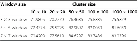
Table 1 Main distance between the central pixel and its neighbors in different windows for different cluster sizes

Window size Cluster size

10 × 10 20 × 20 50 × 50 100 × 100 1000 × 1000

3 × 3 window 71.9805 70.2779 76.4686 75.8885 75.5879

5 × 5 window 72.4774 75.5225 82.9897 82.0059 81.6059

7 × 7 window 70.4209 77.5619 84.6297 83.7486 83.2796

Table 2 Main distance between the central pixel and its neighbors in different windows and original images

Window size Image

Lena Airplane Pentagon Bridge Baboon Boat Pepper Lake

3 × 3 window 5.7539 6.4383 9.0978 14.9330 19.1863 8.6803 5.4787 8.7343

5 × 5 window 7.753 8.4621 10.8822 17.9166 21.6292 11.1673 7.1897 11.9136

Equation (4) is more accurate as the window size increases to 7 × 7 or more. The numbers a and b are the end points of the pixels y’s and equal to 0 and 255, re-spectively. The noisy values y’s are distributed uniformly with meanY. Since xij may take on any value in the

range [0,255], we consider the worst case in which

xij= 0,255. Substituting the values 0 and 255 in

Equa-tion (4), we get the bounds of dc,ij as

0≤dc;ij≤

255

2 ð5Þ

On averagedc,ij= 63.75. Thus, we expect the values of

Dcto be somewhere around the average, as displayed in

Table 1.

For all pixels in the cluster, the average dissimilarities

Dcare calculated as

Dc¼

P_n0 k01 j¼k0

P_m0 l01 i¼l0 dc;ij

n′k01

ð Þ ðm′l01Þ ð6Þ

Values of Dc for different cluster sizes are depicted in

Table 1. It is clear that, these values are almost similar or constant for the different clusters.

Replace n' by n, m' by m, dc,ij by dij, and Dc by D in

Equation (6), and dc,ij by dij in Equation (2). Then, the

Table 3 Comparison for different methods in PSNR (dB)

Method Image

Lena Bridge Baboon Boat Pepper Lake

ACWMF [8] 22.94 23.90 22.05 26.04 25.43 27.50

PWMAD [3] 20.77 22.07 21.33 23.18 22.53 23.66

TSM [7] 20.16 19.45 18.67 21.31 22.12 21.95

MSM [6] 22.21 23.60 22.10 25.58 24.57 26.52

EPRIN [14] 24.90 23.00 20.80 25.48 26.65 27.26

NEW 29.64 24.39 23.27 25.38 29.13 29.50

value ofDfor different original images is calculated and the results are shown in Table 2. One can observe that the difference between the values ofDandDc,as shown

in Tables 1 and 2, respectively, is significant. Such as

Dc>>D ð7Þ

The next step is vital and in which the threshold value

Th is calculated. Threshold helps detecting whether the tested pixel is original or not. Equation (7) suggests that the threshold value should be somewhere between D

and,Dci.e,

D≤Th≤Dc ð8Þ

Dc and D are the average values for different cluster

sizes and different original images, respectively. There-fore, a hard decision threshold is proposed in this article to determine whether the tested pixel is an original or noisy pixel. It is calculated as

Th¼ððDþDcÞ=2Þ ð9Þ

Thus, to detect any pixel xij in the noisy image, the

value of _dijor dc,ijshould be calculated to every pixel in

the image. Pixelxij in the image is considered as a noisy

pixelxnoand flagged asfij= 1 in a binary imageF, ifdijis

more than the threshold value_Th; otherwise is considered original pixelxorand flagged asfij= 0, as shown below

xij¼ xno if dij>Th

xor otherwise

ð10Þ

If the threshold value Th¼ððDþDcÞ=2Þ is selected,

two cases should be considered. In the first case, the

number of the noisy pixels or the clean pixels in the window is less than 50%. In this case, the tested pixel is very likely to be detected correctly, because the majority in the window will be either noisy or clean pixels. In the second case, the number of the noisy pixels in the win-dow is around 50%. Therefore, the probability to detect the tested pixel is rather low. The latter case is more common for pixels located on the edges of the clusters or on the edges of the images. However, the edge pixels of the clusters and the images are small in number com-pared to the total number of the noisy pixels in the clus-ters and to the total clean pixels in the image.

Estimation of the noisy pixels

To estimate the noisy pixels xno’s flagged as fij= 1, the

median value of the good pixels among the neighboring ones in the filtering window is taken. This process runs recursively in the sense that the previously restored pix-els may be used in the restoration of the current pixel. Consider the noisy pixel in the location i,j, then the restored pixelxij,restis attained as

Medij¼medianfωis;jtxis;jtj k0≤s;t≤k0; ðs;tÞ 6¼ ð0;0Þg ð11Þ

xij;rest¼ωijxijþ 1ωij

Medij ð12Þ

ωij¼

0 if fij¼1

1 if fij¼0

ð13Þ

The sign

filtering window may be used in the restoration process, particularly for images corrupted at low noise rate. In addition, different filters such as weighted median filter, center weighted median filter, Gaussian filter, and others may be used instead of the median filter, but all of them provide similarly good results.

Simulation results

It is necessary to carry out extensive experiments to evaluate the performance of the proposed algorithm on different noisy images. The results of the new algorithm are achieved after one iteration for all the simulated experiments and compared with other well-known algo-rithms. The noisy images are produced by corrupting the original ones artificially with many clusters of differ-ent sizes and with continuous and disjoined lines. The readily available images of 512 × 512 size, 7 × 7 window size, MATLAB program, CPU of 1.73 GHz, and 1 GB RAM are used in the simulation experiments. Threshold value used in the simulation is equal to 49, which is very close to the average of the data computed through 7 × 7 window size in Tables 1 and 2, respectively.

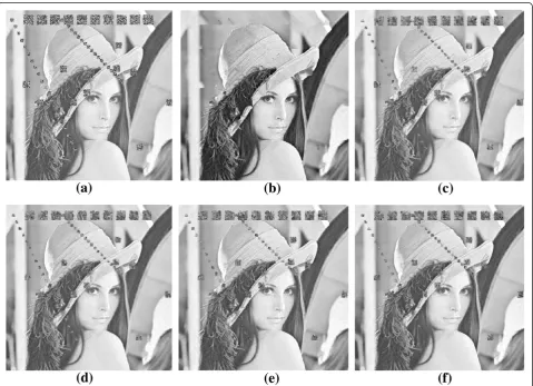
Table 3 and Figure 1 show the performance results of different methods in restoring Lena image, which is corrupted with 40 noisy clusters of 20 × 20 size repre-sented in two lines, 10 clusters of 20 × 20 size, and 10 clusters of 30 × 30 size. These noisy clusters represent 11.6% of all pixels in the image. The simulation proves that the proposed technique delivers the best results among the other methods either in terms of PSNR, as indicated in Table 3, or with regard to visual quality, as indicated in Figure 1. It is obvious that the proposed method has efficiently restored the noisy clusters, while the other methods have failed. Remarkably, 96.9% of the clusters pixels are detected correctly as noisy pixels, and 1.267% of the original pixels are detected wrongly as noisy pixels. Figure 2 shows the locations of the pixels that are detected wrongly. Apparently, these pix-els are located either on the clusters edges or on the image edges.

While the number of the noisy pixels in the different clusters in Lena image is small compared to the total

number of the pixels in the image, it should be added that detecting and restoring noisy clusters are more diffi-cult than restoring noisy pixels spread over the image. In other words, restoring scattered noise, small-sized clus-ters, or thin lines of noisy pixels is easier than restoring clusters of larger size or thick lines.

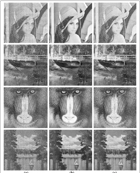
Figure 3 and Table 4 show the restoration results in terms of visual quality and PSNR, respectively, for differ-ent algorithms in restoring images corrupted with 2,601 clusters each of 5 × 5 size. The ratio of the noisy pixels in all the clusters compared to the total number of the pixels in each image is 26%.

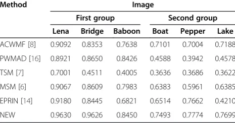
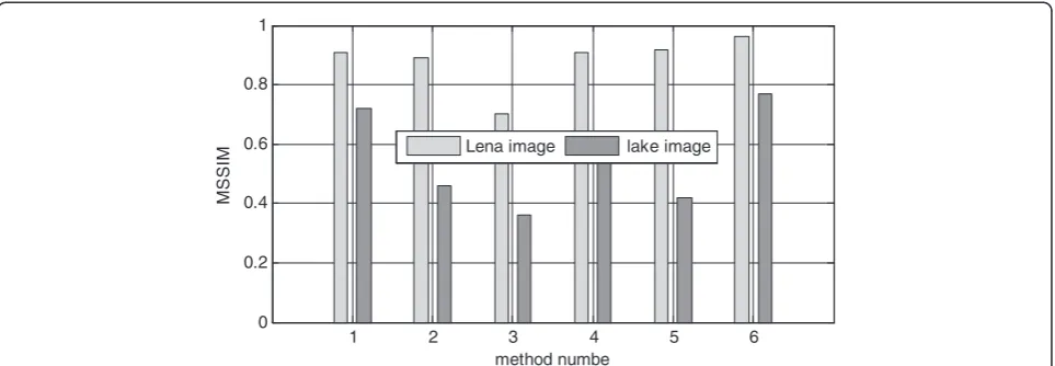
Table 5 shows the restoration performance in terms of Mean Structural Similarity (MSSIM) for different meth-ods in restoring two groups of corrupted images. The first group includes Lena, bridge, and baboon images degraded by the same noisy clusters shown in the cor-rupted Lena image in Figure 1. Namely, 40 noisy clusters of 20 × 20 size represented in two lines, 10 clusters of 20 × 20 size and 10 clusters of 30 × 30 size corrupt the images. The other group includes images of boat, pep-per, and lake, which are degraded by the same noisy clusters shown in the corrupted images in Figure 3. Figure 4 compares the restoration performance of dif-ferent methods in restoring the corrupted images of Lena and lake depicted in Figures 1 and 3, respect-ively. Results are shown visually and numerically in terms of MSSIM.

As the previous figures and tables show, the proposed method illustrates superior results to other techniques either objectively in terms of PSNR and MSSIM, or sub-jectively as demonstrated in the restored images. The values of PSNR and MSSIM that are achieved by the new method are clearly better than the other known methods. In addition, the images restored with the help of the proposed algorithm are free of noise, stains, or spots. Therefore, the proposed method is efficient and shows high level of restoration performance. Further-more, the proposed algorithm is very fast since during the first and second experiments (Figures 1 and 3), the new method consumes almost the same processing time

Table 4 Comparison for different methods in PSNR (dB)

Method Image

Lena Bridge Baboon Boat Pepper Lake

ACWMF [8] 22.1727 21.7124 20.3953 23.9013 24.5486 24.4295

PWMAD [3] 17.4493 18.2942 17.7662 19.1667 19.2392 19.5295

TSM [7] 17.5533 17.7064 17.0609 19.1884 19.7068 19.6355

MSM [6] 19.9696 20.6734 19.6719 22.2229 22.4310 22.8236

EPRIN [14] 22.7913 22.0507 17.4171 21.3431 26.0712 19.2907

NEW 26.4716 22.4947 21.7610 23.7811 26.5883 26.0173

Table 5 Comparison for different methods in MSSIM

Method Image

First group Second group

Lena Bridge Baboon Boat Pepper Lake

ACWMF [8] 0.9092 0.8353 0.7638 0.7101 0.7004 0.7188

PWMAD [16] 0.8921 0.8650 0.8426 0.4588 0.3942 0.4578

TSM [7] 0.7001 0.4511 0.4005 0.3636 0.3686 0.3622

MSM [6] 0.9067 0.8609 0.7983 0.6383 0.5961 0.6385

EPRIN [14] 0.9180 0.8445 0.6821 0.6514 0.7662 0.4210

that is consumed by well-known filters as ACWMF [8] and MSM [6].

Conclusion

The novel algorithm proposed in this article is based on the differences in the illumination levels among the pix-els in the noisy images. Illumination values make it pos-sible to differentiate between the noisy and clear pixels. The new method allows the identification and elimin-ation of the cluster pixels, and has proven to have a su-perior performance in terms of PSNR, MSSIM, and perceptual image quality. Finally, the new method is easy to implement and has low computational complexity.

Competing interests

The author declares that he has no competing interests.

Acknowledgments

I would like to express my gratitude to the reviewers and to the associated editor for their valuable comments and to anyone who helping me in producing this article.

Received: 4 January 2012 Accepted: 5 July 2012 Published: 25 July 2012

References

1. J. Wu, C. Tang, PDE-based random-valued impulse noise removal based on new class of controlling functions. IEEE Trans. Image Process.

20(9), 2428–2438 (2011)

2. U. Ghanekar, A.K. Singh, R. Pandey, A contrast enhancement-based filter for removal of random valued impulse noise. IEEE Signal Process. Lett.17(1), 47–50 (2010)

3. V. Crnojevi’c, V. Senk, Z. Trpovski, Advanced impulse detection based on pixel-wise MAD. IEEE Signal Process. Lett11(7), 589–592 (2004) 4. A.S. Awad, Standard deviation for obtaining the optimal direction in the

removal of impulse noise. IEEE Signal Process. Lett.18(7), 407–410 (2011) 5. R.H. Chan, C. Hu, M. Nikolova, An iterative procedure for removing

random-valued impulse noise. IEEE Signal Process. Lett.11(12), 921–924 (2004) 6. T. Chen, H.R. Wu, Space variant median filters for the restoration of impulse

noise corrupted images. IEEE Trans. Circuits Syst. II48(8), 784–789 (2000) 7. T. Chen, K.K. Ma, L.H. Chen, Tri-state median filter for image denoising. IEEE

Trans. Image Process.8(12), 1834–1838 (1999)

8. T. Chen, H.R. Wu, Adaptive impulse detection using center-weighted median filters. IEEE Signal Process. Lett.8(1), 1–3 (2001)

9. W. Luo, D. Dang,An efficient method for the removal of impulse noise (Proceedings of IEEE International Conference on Image (ICIP), Atlanta, Georgia, USA, 2006), pp. 2601–2604

10. M. Emin Yüksel, A. Baştürk, E. Beşdok, Detail-preserving restoration of impulse noise corrupted images by a switching median filter guided by a simple neuro-fuzzy network. EURASIP J. Appl. Signal Process

16, 2451–2461 (2004)

11. W. Luo, D. Dang, A new directional weighted median filter for removal of random-valued impulse noise. IEEE Signal Process. Lett.14(3), 193–196 (2007)

12. R. Garnett, T. Huegerich, C. Chui, W.-J. He, A universal noise removal algorithm with an impulse detector. IEEE Trans. Image Process.

14(11), 1747–1754 (2005)

13. Y. Dong, R.H. Chan, S. Xu, A detection statistic for random-valued impulse noise. IEEE Trans. Image Process.16(4), 112–1120 (2007)

14. H. Yu, L. Zhao, H. Wang, An efficient procedure for removing random-valued impulse noise in images. IEEE Signal Process. Lett15, 922–925 (2008) 15. T. Mélange, M. Nachtegael, E.E. Kerre, Fuzzy random impulse noise removal

from color image sequences. IEEE Trans. Image Process.20(4), 959–970 (2011)

16. L. Shao, J. Wang, I. Kirenko, G. de Haan, Quality adaptive least squares filters for compression artifacts removal using a no-reference block visibility metric. J. Visual Commun. Image Represent.22(1), 23–32 (2011)

17. L. Shao, H. Zhang, G. de Haan, An overview and performance evaluation of classification based least squares trained filters. IEEE Trans. Image Process.

17(10), 1772–1782 (2008)

18. L. Shao, Up-scaling images in presence of salt and pepper noise. IEE/IET Electron. Lett.43(14), 746–748 (2007)

doi:10.1186/1687-6180-2012-161

Cite this article as:Awad:Localizing and restoring clusters of impulse noise based on the dissimilarity among the image pixels.EURASIP Journal on Advances in Signal Processing20122012:161.

1 2 3 4 5 6

0 0.2 0.4 0.6 0.8 1

method numbe

M

SSIM

Lena image lake image

Figure 4Comparison between the proposed method and other known algorithms for restoring corrupted Lena and lake images in