R E S E A R C H
Open Access
Dimension expansion and customized spring
potentials for sensor localization
Jieqi Yu
*, Sanjeev R Kulkarni and H Vincent Poor
Abstract
The spring model algorithm is an important distributed algorithm for solving wireless sensor network (WSN) localization problems. This article proposes several improvements on the spring model algorithm for solving WSN localization problems with anchors. First, the two-dimensional (2D) localization problem is solved in a
three-dimensional (3D) space. This “dimension expansion” technique can effectively prevent the spring model algorithm from falling into local minima, which is verified both theoretically and empirically. Second, the Hooke spring force, or quadratic potential function, is generalized intoLppotential functions. The optimality of different values ofp is considered under different noise environments. Third, a customized spring force function, which has larger strength when the estimated distance between two sensors is close to the true length of the spring, is proposed to increase the speed of convergence. These techniques can significantly improve the robustness and efficiency of the spring model algorithm, as demonstrated by multiple simulations. They are particularly effective in a scenario with anchor points of longer broadcasting radius than other sensors.
1 Introduction
Localization is an essential tool in many sensor network applications. Over the years, a rich literature has been developed to solve the sensor localization problem from different perspectives [1-3]. Franceschini et al. character-ized them according to four criteria in their survey article [1]: anchor-based vs. anchor free, incremental vs. concur-rent, fine-grained vs. coarse-grained, and centralized vs. distributed.
In this article, we propose several techniques to improve the robustness and computational efficiency of an anchor based, concurrent, fine-grained, and distributed spring-model-based sensor localization algorithm. We start our discussion by reviewing several representative distributed sensor localization algorithms.
2 Related study
Savarese et al. [4] proposed an incremental and anchor-based localization algorithm that uses a two-phase approach, including an initial position estimation stage
*Correspondence: [email protected]
Department of Electrical Engineering, Princeton University, Princeton, NJ 08544, USA
and a second stage for position refinement using trilater-ation. It is accurate compared to traditional incremental methods, which are prone to error propagation. How-ever, the method can produce dramatically incorrect node displacement when measurement noise is present.
To increase accuracy in a noisy environment, Moore et al. [5] argue that measurement noise can cause flip ambiguities during trilateration. They proposed a robust incremental algorithm, dramatically reducing the amount of error propagation. However, this algorithm has rela-tively high computational complexity and its third stage can hardly be handled without a centralized node [1]. Fur-thermore, Franceschini et al. [1] points out that, under large measurement noise, the algorithm may fail to local-ize enough nodes.
Ihler et al. [6] proposed a distributed localization algo-rithm from a different perspective. It is based on graph models and requires a prior distribution for the sensor locations. It is accurate and fully distributed. Furthermore, in [7], a graph model based cooperative algorithm is pro-posed and tested with real measurements. The algorithm requires knowledge of the distributions of range measure-ments between pairs of sensors. However, prior knowl-edge of the sensor deployment and range distribution might not be available in many applications.
Algorithms based on machine learning techniques have also been proposed [8,9]. These algorithms typically assume that a large number of anchor points are present, which is impractical in many cases.
The algorithms reviewed above are all range-based algorithms. The range information in sensor networks can be obtained with various methods, such as time of arrival (TOA) based ranging techniques, even for mul-tipath environments [10]. Nonetheless, many methods also try to take advantage of additional/alternative infor-mation beyond range/distance measurements, including sector/bearing information [11], information about con-nectivity among sensor nodes [12], information about connectivity to anchor nodes [13] and measurement errors (vertex errors and edge errors) [14].
These methods use the additional/alternative informa-tion above to improve accuracy, accelerate convergence and reduce computational complexity. Because of the diversity of information available for sensor network local-ization, Shen et al. proposed a theory to quantify the limits of localization accuracy for wideband wireless networks in [15] and [16], by introducing the concept of squared position error bound.
Priyantha et al. [17] proposed a two stage anchor-free distributed algorithm (AFL). The first stage, the initial-ization stage, produces a qualitative network node graph, while the second stage refines the result by using a spring model, which is the most relevant to our algorithm.
In the spring model method, any pair of sensors with knowledge of mutual distance are considered to be nodes connected by a spring of the same length. The force each spring applies to the nodes depends on the difference between inter-node estimated distances and actual dis-tances. Given sufficient connections amongst the sensors, the system has a unique zero-energy state with all the sensors in correct relative position, up to global transi-tion, rotation and mirror transformation. Furthermore, if enough anchor nodes (sensors with knowledge of their true coordinates) are introduced, the absolute coordinates of the sensors can also be estimated.
One of the advantages of the spring model is the ease with which it can be implemented as a fully distributed algorithm, i.e., each sensor needs to communicate only with its neighbors, repeatedly updating its estimated loca-tion until convergence. However, there are several draw-backs to the spring model.
The most prominent problem is the “folding” phe-nomenon in which the spring system falls into an energy local minimum and cannot unfold itself. To tackle this problem, many pre-processing methods have been pro-posed, such as the first stage of the AFL algorithm, which may fail due to an insufficient number of nodes or to mea-surement noise. Gotsman et al. [18] improved the first stage of the AFL algorithm, by solving an eigenvector
problem. It can be distributized, but requires many itera-tions, thus incurring significant communication cost.
Another problem with the spring model (with Hooke’s law) is that the potential energy, measured by the squared error between the true distance and the estimated dis-tance, is sensitive to measurement error, and hence is not robust enough for many applications.
Moreover, in [17] and [18], all scenarios are established on relative coordinates with no anchor. In the case of the presence of anchors, or if absolute coordinates are required, another round of information propagation is needed to transform the coordinates of each sensor to the corresponding absolute coordinates.
In this article, we propose a new spring-model algo-rithm to resolve the problems mentioned above with the presence of anchors. First, we solve a two-dimensional (2D) sensor localization problem in a three-dimensional (3D) space, which significantly reduces the occurrence of “folding”. This algorithm requires no preprocessing, and operates in a distributed manner, which converges with competitive rate compared to algorithms in [17] and [18]. Moreover, to improve the noise resistance of the algorithm to range measurement noise, we investigate the estimation error of different types of spring potential functions under different noise distributions. Furthermore, we design a customized spring force so that the spring has a larger strength coefficient once the estimated distance between two sensors is close to the measured distance between them. This customized spring can effectively accelerate the convergence speed of the system and also reduce the estimation error.
The rest of this article is organized as follows. In Section 3, the spring model sensor localization problem is defined. In Section 3.2, a distributed algorithm is proposed to solve the spring model sensor network localization prob-lem. The idea of dimension reduction is explained and simulated in Section 4. In Section 5, the optimal spring potential function under different noise distributions is explored via extensive simulations. In Section 6, a cus-tomized spring force is proposed to increase convergence speed as well as to reduce estimation error, and Section 7 concludes our article.
3 Spring model with anchors
3.1 Basic model
difference between the measured distance and the esti-mated distance is defined by the potential function
Eij=P
xi−xj −dij
, (1)
then the localization problem can be described as
arg minxi,i=1,...,N1 2
N
i=1
j∈Ni(r)
Pxi−xj −dij
. (2)
Assume thatAis the set of indices of the anchor sen-sors; then their coordinates should be excluded from the variables of the optimization problem. Therefore, (2) can be specialized as
arg minxi,i∈Ac
1 2
N
i=1
j∈Ni(r)
Pxi−xj −dij
, (3)
given{xi,i∈A}known and fixed.
Next, we will introduce an iterative, distributed algo-rithm that solves (2), and further specialize this algoalgo-rithm to solve its derived problems for different network config-urations and noise types.
3.2 Distributed algorithm solving the spring model for sensor localization
The basic idea of the spring model is to run the system in a physical world with energy dissipation until it reaches its lowest potential state. Each sensor is deemed to be a ball of massmand negligible size, and the entire system is immersed in a damping liquid of viscosityβ. At time
t, each sensor is pushed/pulled by the force exerted by the tension of the spring connected to its neighbors, and also dragged by the damping force opposite to its velocity. Under these assumptions, a distributed, iterative algo-rithm is proposed to find a solution to (2). The algoalgo-rithm is summarized as Algorithm 1 below:
The basic idea of Algorithm 1 is to set up a physical environment with appropriate damping for the system to run freely until the kinetic and elastic potential energy dissipates. The steady state of the system is a local min-imum of the objective function, which is likely to be the desirable solution of the localization problem. The conver-gence to the global minimum is not guaranteed. However, with proper control of parameters and wise choice of the initial condition, we can improve the possibility of success.
Algorithm 1 Distributed algorithm for spring model whileTermination Condition isfalse do
/∗Local Communication Stage∗/
fori∈ {1,. . .,N}do
Sensori collects{xj,j∈Ni(r)}from its
neighbors
end
/∗Local Computation Stage∗/
fori∈ {1,. . .,N}do ai←j∈Ni(r)
p(xi−xj−dij) m
xj−xi xj−xi−
βvi m
end
fori∈ {1,. . .,N}do vi←vi+ait
xi←xi+vit
end end
Moreover, Algorithm 1 is purely distributed. There are two stages in the algorithm:
1. Local communication stage: Each sensor collects the current estimates of the coordinates from its neighbors. This process is purely local within the radiusr.
2. Local computation stage: Each sensor updates the estimate of its coordinates (and corresponding virtual speed and acceleration) based on the information collected locally.
Most importantly, this model is highly configurable by setting the mass, viscosity, spring strength, and spring force type of the system. Next, we will discuss a special formulation that introduces anchor nodes into the system.
3.3 Introducing anchors: long-range anchor scenario
Intuitively, when the anchors’ coordinates are known accurately, they can be deemed to be ordinary sensor nodes, except with infinite mass, so that they will not update their coordinates. When the anchors’ coordinates are known up to a confidence level, they can be modeled as ordinary sensors, connected to an imaginary anchor (with infinite mass and set at the believed location) by a hard spring, with strengthkmuch higher than others, reflect-ing the confidence level of the anchor in its coordinates. In our simulations, we assume that the anchors have accu-rate absolute coordinates, and hence do not update their own coordinates at all.
Moreover, since the anchors do not need to update their coordinates, they are not part of the iterative algorithm. Their only task is to broadcast their coordinates and dis-tance measurements to their neighbors once. This gives rise to an interesting scenario, discussed next, in which the anchors have longer broadcasting ranges than ordinary sensors.
for more sensors to know their distances to at least one anchor, and this can greatly accelerate the speed at which anchor information spreads throughout the network.
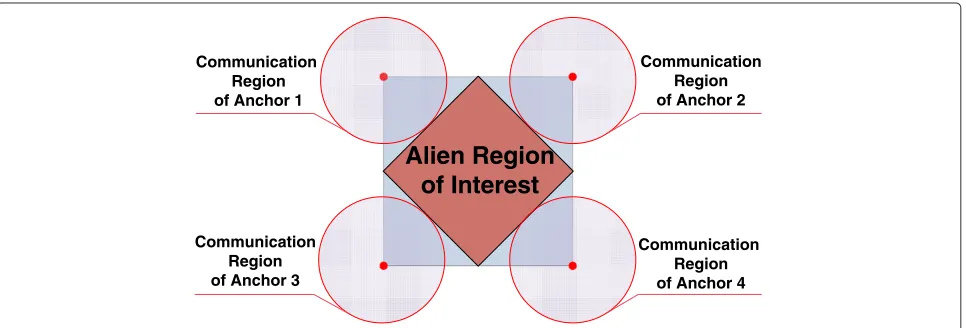
Following the arguments described previously, we intro-duce a scenario shown in Figure 1, in which the four anchors have longer communication ranges than ordi-nary sensors, and do not enter into the iterations of the algorithm.
In Figure 1, the four anchors are located at the four vertices of the unit square, with communication radii approximatelyranchor = 0.35. All the other sensors have
a smaller communication radii of r = 0.1. The red
region is completely out of the range of anchors. Simula-tions in Section 6, in which we combine all techniques to improve the spring model algorithm for sensor localiza-tion, employ this configuration.
4 Dimension expansion
4.1 “Folding” phenomenon and dimension expansion
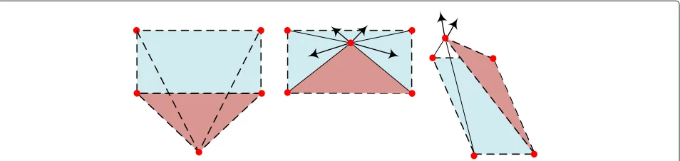
The most prominent problem when running Algorithm 1 is the “folding” phenomenon. In a 2D space, two parts of the system could fold together, with a few springs strained, becoming stuck in an energy local minimum. Figure 2 illustrates a typical example of the folding phenomenon.
For example, in Figure 2, the left graph represents the global minimum, yet the middle graph is a “folding” sce-nario, with four springs strained. Unfortunately, once the spring system falls into a folding local minimum in a 2D space, it is rather difficult for the system to resolve on its own, without external perturbation, since all forces are within the same plane. However, if the 2D spring system is allowed to evolve in a 3D space, a small displacement in the third dimension can effectively unfold the system that falls into a “folding” local minimum, as shown in the right part of Figure 2. We refer to this technique as dimension expansion.
By initializing the third dimension of the sensor coordi-nates according to a uniform distribution, the probability of the “folded” sensors lying exactly on the same 2D plane is zero. As a result, dimension expansion can resolve many folding scenarios and hence circumvent local minima (more detailed discussion can be found in Section 4.2). Moreover, since the anchors are located on the same 2D plane, the global minimum of the relaxed system remains the same as the original problem (given that all the dis-tance measurements are accurate), with all the sensors lying in the same 2D plane as the anchors.
However, the benefits come with a price. First, compu-tationally, dimension expansion adds one more coordinate that the sensors need to maintain and communicate. Sec-ond, with measurement noise, this may cause the third dimension to overfit to the noise.
Nonetheless, our simulations demonstrate that the dimension expansion technique has almost the same con-vergence rate as its 2D counterpart while significantly reducing the chances of “folding”, and performs well for large noise scenarios when there is a sufficient number of anchor points. These properties will be demonstrated via simulations next and in Section 6.
Before demonstrating more empirical results, we will first explore a simple case of a three-body scenario to explain the theoretical foundation of the efficacy of dimension expansion.
4.2 Why dimension expansion works
Although simulations in later sections will confirm our intuition that dimension expansion resolves the “folding” problem, in this section we provide a mathematical expla-nation of this intuition to better understand the capability and limitations of dimension expansion.
Since the derivation is very intricate for high dimen-sional cases, in this subsection, we illustrate the math-ematical foundation of dimension expansion using a 1D
Alien Region
of Interest
Communication Region of Anchor 2 Communication
Region of Anchor 1
Communication Region of Anchor 3
Communication Region of Anchor 4
Figure 2Illustration of the folding phenomenon.Left: correct displacement of the sensors, global minimum; middle: folding phenomenon, system reaches local minimum—forces within the 2-D space cannot unfold the system; right: the system unfolds easily with the introduction of the third dimension.
to 2D expansion with a three-body model. Although this simplified model has some differences from our 2D to 3D simulation and application, it still sheds some light on the fundamental ideas of dimension expansion.
4.2.1 Model and setup
Suppose that we have three balls numbered 1, 2, and 3. They are connected by springs of intrinsic lengthsl12,l13, andl23. Without loss of generality, we assume thatx1 < x2 < x3, wherexidenotes the coordinate of theith ball. Under the assumption that the three balls are confined in a 1D space and there is no observational error, we have an extra constraint
l12+l23=l13. (4)
Therefore, the elastic potential energy of the entire system can be expressed as
L(x1,x2,x3)=
1≤i<j≤3 k
2(|xi−xj| −lij)
2. (5)
In the globally optimal state, i.e., when the “correct” configuration of the relative positions of the balls are reached, the potential energy in (5) is 0. However, it can be shown that, if the balls are confined in 1D, then there exist stable configurations that are not globally optimal (i.e., they are local minima), and hence lead us to “incor-rect” configurations if we use the spring model without discretion.
4.2.2 Existence of stable suboptimal equilibrium (SSE)
Without loss of generality, we assumek =2,l13 = 1 and l12=α, in which 0< α <1. According to (4),l23=1−α. Any equilibrium configuration of the system needs to satisfy
∂L
∂xi =
0,∀i∈ {1, 2, 3}. (6)
Hence, by substituting (5) into (6), we obtain
⎧ ⎪ ⎨ ⎪ ⎩
2x1−x2−x3−l12sgn(x1−x2)−l13sgn(x1−x3)=0
2x2−x1−x3−l12sgn(x2−x1)−l23sgn(x2−x3)=0
2x3−x1−x2−l13sgn(x3−x1)−l23sgn(x3−x2)=0
.
(7)
Equations (7) provide us with the necessary condition for a stable equilibrium. However, to sufficiently guar-antee that an equilibrium is stable, we also need the Hessian matrix of L(x1,x2,x3) to be semi-positive defi-nite. By deriving the second-order partial derivatives of
L(x1,x2,x3), we obtain ∂2L
∂x2i =2−2
j =i
lijδ(xi−xj) (8)
and
∂2L
∂xi∂xj = −1+
2lijδ(xi−xj), i =j, (9)
whereδis the Dirac delta function, andi,j∈ {1, 2, 3}.
From (8) and (9), we can conclude that as long as (7) does not yield solutions for which
∃(i,j) s.t.xi=xj, (10)
the Hessian matrixH(x1,x2,x3)is a constant matrix
H(x1,x2,x3)= ⎡ ⎢ ⎣
, 2 −1 −1
−1 2 −1
−1 −1 2
⎤ ⎥
⎦. (11)
The Hessian matrix in (11) is semi-positive definite, which guarantees that almost any equilibrium given by the solution of Equation (7) is stable, as long as condition (10) is not satisfied. Therefore, we can solve (7) to show that sub-optimal solutions do exist.
x1=0. Then, there are three unique non-trivial scenarios excluding symmetric equivalent ones:
• Scenario 1:0<x2<x3; • Scenario 2:0<x3<x2; • Scenario 3:x2<0<x3.
Compared to Scenario 1, which has the global optimum as the solution to (7), i.e.,
x2=α, x3=1, (12)
Scenarios 2 and 3 are more of interest to us. Under the assumption of Scenario 2, the solution to (7) turns out to be
x2= α+ 2 3 , x3=
2α+1
3 . (13)
Obviously,x2 = x3, so (13) is a stable equilibrium, which is a concrete example of the “folding phenomenon” in 1D space. Similarly, we can find the solution in Scenario 3 as
x2= −α
3,x3=1− 2α
3 . (14)
By arguments similar to that for Scenario 2, (14) is also a stable equilibrium.
Therefore, we have shown the existence of stable sub-optimal equilibrium (SSE) configurations for the three body spring model in 1D space.
4.2.3 Eliminating SSEs by dimension expansion
Although SSEs exist for the three body model in 1D space, they can be eliminated by dimension expansion, which, in this case, is to allow the 1D system to evolve in a 2D space. Denoting the coordinates of the balls by (xi,yi), i ∈ {1, 2, 3}, the potential function in (5) can then be rewritten as
Lx1,x2,x3,y1,y2,y3
=
1≤i<j≤3 k
2(
(xi−xj)2+(yi−yj)2−lij)2
(15)
The standard method to find out all equilibria for (15) is to solve the six equations derived from
∂L
∂xi =
0,∀i∈ {1, 2, 3}
∂L
∂yi =
0,∀i∈ {1, 2, 3}.
However, a simple argument can save us the effort: We claim that the three-body spring model has an equivalent set of equilibria in 2D space, as in 1D space, with possible changes in stability.
The reasoning behind this claim is as follows. First, notice the fact that each ball in the three-body system is pulled/pushed by exactly two springs. For each ball to
be in equilibrium, the two forces must both be 0, or co-linear. The former situation is achieved only in the unique globally optimal state, in which the three balls are co-linear. Therefore, the three balls must always be co-linear (located in a 1D space) in any equilibrium, and hence the 2D equilibrium solutions must be equivalent to the 1D ones.
Although the 2D equilibria are equivalent to the 1D ones, the stability of those equilibria may not necessarily be the same. And the essence of dimension expansion is to expand the system into a higher dimension so that the sta-ble local optimal configurations in the lower dimensional space become unstable in the higher dimensional space, which is exactly what happens in this case.
To investigate the stability of an equilibrium, we need to investigate the semi-positive-definitness of the Hessian matrix at the equilibrium. To show that the Hessian matrix is no longer semi-positive definite, it is sufficient to show that one of the diagonal element of the Hessian matrix is negative.
Let us first take Scenario 2 as an example. Without loss of generality, we assume that the equilibrium hasy1 = y2 =y3 = 0. Further assumingk =2, from (15), we can derive
∂2L ∂y21
=2− l12(x1−x2) 2
(x1−x2)2+(y1−y2)2
− l13(x1−x3)2 (x1−x3)2+(y1−y3)2
.
(16)
Substituting x1,x2,x3,y1,y2,y3 from the solution of Sce-nario 2, which is
x1=0,x2= α+ 2 3 ,x3=
2α+1
3 ,y1=y2=y3=0, we obtain
∂2L ∂y21
= −2 (α−1)2
(α+2)(2α+1), (17)
by the assumption that 0 < α < 1. Therefore (18) is strictly less than 0, which means that the Hessian matrix for the equilibrium in Scenario 2 is no longer stable. Con-sequently, by dimension expansion from 1D to 2D, we eliminate an SSE configuration of the three-body system.
A geometric explanation of this phenomenon is that, in 1D space, an equilibrium can be a stable local optimum, while in the 2D situation, the local optimum becomes a saddle point.
Similarly, by substituting x1,x2,x3,y1,y2,y3 from the solution of Scenario 3, we obtain
∂2L ∂y21
= −1− 1
3−2α, (18)
Therefore, both SSE configurations are unstable in the 2D case, which leaves us with a unique solution—the desired global optimum.
4.2.4 Conclusions
With the analysis on 1D to 2D dimension expansion using a three-body model, we have come up with two important conclusions:
1. For a 1D three-body spring model with no measurement noise, the “folding phenomenon” always exists, since there are two non-trivial SSE configurations; and
2. If we expand the space from 1D to 2D, all the SSE configurations become unstable and the system will evolve into the unique globally optimal configuration.
Although the model for the analysis above is simple com-pared to more general cases, the conclusion is quite insightful: by allowing the system to have one more degree of freedom, the local optima are converted into saddle points and hence eliminated, which is the essence of dimension expansion.
To further demonstrate the efficacy of dimension expan-sion in more general cases, we resort to numerical simu-lations in the following section.
4.3 Efficacy of dimension expansion
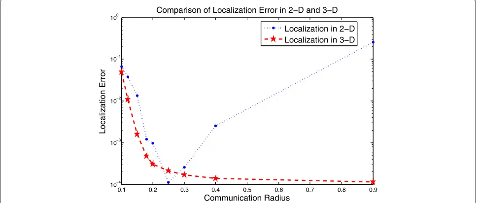
The theoretical model only shows us the situation in the 1D/2D case with a simple three-body model. To fully explore the capability of dimension expansion, we com-pare the performance of the spring system with and without dimension expansion in a 2D/3D configuration.
We assume that the springs obey Hooke force in the experiment, i.e., the potential function isp(x)=kx2.N=
500 sensors are scattered at random in a 1×1 2D square. On each vertex, the midpoint of each side, and the center of the square, there is an anchor (a total of 9). Assuming all measurements of distance within communication radius
rare accurate, we run a series of simulations for different values ofr, withm= 1 for all sensors,k= 5,t =0.01, andβ = 1, wheremis the mass of the sensor, andβ is the viscosity of the liquid, as described in Section 3. The simulation results are shown in Figure 3.
The initial location of each sensor is a uniformly dis-tributed random point in the unit square. For the 3D algorithm, the coordinate for the third dimension is ini-tialized as a uniformly distributed value on [−0.1, 0.1]. Assuming that x0i is the true location of sensor i, the localization errorEis measured by
E =
1
N
N
i=1
xi−x0i2.
For small values ofr, some sensors do not have sufficient constraints to specify their absolute coordinates. Hence, both 2D and 3D algorithms have large estimation errors. Whenrgrows larger, the 3D algorithm performs very well, consistently converging to the desired global minimum. However, as the links among the sensors increase, the 2D algorithm has many chances to fall into local minima and hence incurs a large estimation error. Therefore, this experiment confirms the efficacy of dimension expansion. Another important issue is the convergence speed. As is common for many optimization algorithms, the selection
0.1 0.2 0.3 0.4 0.5 0.6 0.7 0.8 0.9
10−4 10−3 10−2 10−1 100
Communication Radius
Localization Error
Comparison of Localization Error in 2−D and 3−D
Localization in 2−D Localization in 3−D
of parameters is essential to the convergence speed. The value ofkandmcan be selected arbitrarily, because the effect of ratiok/mcan be compensated by the choice ofβ andt. The choice oftshould follow the general rules for choosing step sizes for optimization problems: too large of atleads to poor accuracy in the vicinity of the optimal region, and too small of atresults in very slow convergence. Lastly,βis chosen following the guidance of damped harmonic oscillation of springs. Largeβ leads to over-damping, which results in slow convergence and sus-ceptibilities to local minimum; on the other hand, small β leads to under-damping, which causes a long time of oscillation and slow convergence. In practice,βis selected slightly less than the critical damping factor 2k/m(in our set up, the critical damping factor is approximately 4.47, and β is chosen as 1), to avoid unnecessarily pro-longed oscillation, while provide the system with enough freedom to avoid bad local minima.
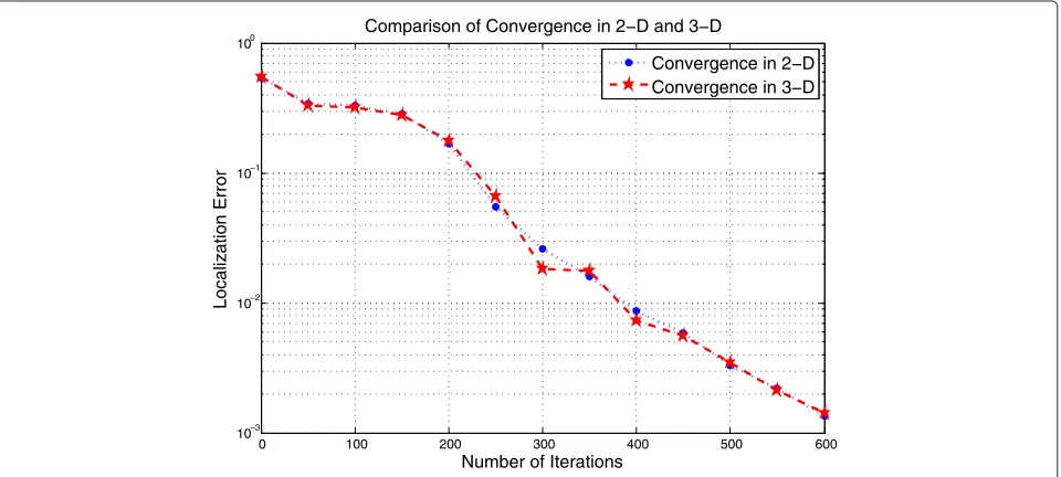
Figure 4 compares the convergence rates for the case
of N = 1000 andr = 0.15, for both 2D and 3D
algo-rithms. The graph shows that they converge at similar speeds despite the fact that the 3D algorithm has one more dimension.
In these and other examples, we find that the 3D algo-rithm, though having one more dimension, does not have an observable disadvantage in terms of the rate of reduc-ing the localization estimation error.
5 Optimal spring potential
Besides changing the dimension of the space in which we run the algorithm, the distributed spring model algorithm also has the advantage that it can easily adapt to different types of noise, with the mere change of the force/potential
(use non-Hooke force). Various types of potentials can be designed to adapt to different types of noise.
To simplify the problem, in this section, we analyze the group of potentials of the form
Eij=Pxi−xj −dij=xi−xj −dijp, (19)
wherep≥1, to identify the optimal spring potential, i.e., we seek optimal values of p, for different types of noise. For simplicity, we henceforth call the potential function represented in Equation (19) theLppotential.
Let us first consider a simplified model withNanchors and only one sensor to be localized, with noisy dis-tance/range measurements. Let Ai,i = 1,. . .,N, be anchors located uniformly on a unit circle in two dimen-sional space, with locations denoted as xAi,xAi = 1.
Suppose the only sensor to be localized,S, is located at the center of the circle. The distance measurements between
Sand the anchorsAi,i=1,. . .,N, are corrupted by differ-ent types of noise with mean 0 and standard deviationσ.
Given the range measurements andxAi,i = 1,. . .,N,
sensorScan easily estimate its location,xS, using the dis-tributed spring model algorithm described in Section 3, with the desired force/potential. For each specific type of noise and potential, sensor S solves the following opti-mization problem:
min xS
N
i=1
xAi−xS −(1+ξi)p, (20)
where ξi,i = 1,. . .,N, are independent and identically distributed (i.i.d.) random variables with means 0 and standard deviationsσ.
0 100 200 300 400 500 600
10−3 10−2 10−1 100
Number of Iterations
Localization Error
Comparison of Convergence in 2−D and 3−D
Convergence in 2−D Convergence in 3−D
Given a particularpand the joint distribution ofξi,i=
1,. . .,N, the optimization result of (20) forms a distribu-tion distp(xS). In order to investigateLp potentials with different values ofp, we compare the group of distribu-tions distp(xS),p ≥ 1, to find the optimal potential, in terms of accuracy, for different types of noise.
Intuitively, we desire the distribution distp(xS) to con-centrate around the origin as closely as possible. Specif-ically, we desire a potential function, as specified by parameterp, that has a spiky distp(xS) centering around the true location(0, 0), since this demonstrates the robust-ness of the spring potential to resist noise. Therefore a nat-ural measure of the performance would be theq-quantile of the distributions of the distance from our estimate to the true location, and deem the potential with smallest
q-quantile distribution theq-optimalLppotential for the particular noise.
To be more specific, the distance from our estimate to the true location(0, 0) is simplyxS; so from the dis-tribution function ofxS, i.e., distp(xS), we can derive the distribution ofxS, i.e.,
p(r)=P{xS ≤r}. (21)
For a given system and noise distribution, the distribu-tion funcdistribu-tion p(r)is a function of the parameterponly. Therefore, theq-optimal value ofpis defined as
p∗=arg minp −p1(q), (22)
where −p1(q)is the inverse function of the distribution function ofxS.
Since the optimization problem (20) is non-convex, it is difficult to find the analytical form of distp(xS) and
thus theq-optimal spring potential. Therefore we turn to numerical methods to investigate theq-optimal potential for different types of noise.
In the numerical experiments, N anchors are
fixed uniformly on the unit circle, with coordinates (cos2Nπi, sin2Nπi). Then, a large number of rounds of sim-ulations are run to generate the distribution distp(xS)for a specific p. At each round, the distance measurements betweenSand the anchorsAi,i=1,. . .,N, are corrupted by the desired additive noise. In order to find the local-ization result of sensorS, i.e., the global minimum of the optimization problem (20), we search in fine grids within the square circumscribed about the unit circle. The total number of times each grid point becomes the global minimum in all rounds are counted, and the distribution distp(xS) is then represented by the frequency of “hits” received at each grid point.
Figure 5 shows the setting and resulting distp(xS) of a particular run of the experiment, where p = 2. In this experiment, the range measurements are corrupted by additive Gaussian noise, with mean 0 and standard devia-tion 0.2. Ten anchors are used and ten thousand rounds of simulations are run to generate the distribution dist2(xS), in which, at each round, a 100-by-100 grid is searched for the global minimum of (20).
On the left hand graph of Figure 5, ten dots on the unit circle show the positions of the anchors, while color rep-resents the number of “hits” received by each grid point. The right hand graph is a 3D mesh plot of the left hand graph, which shows dist2(xS)under Gaussian noise.
Given distp(xS)represented by the frequency of “hits” received at each grid point, the distribution function
−1 −0.8 −0.6 −0.4 −0.2 0 0.2 0.4 0.6 0.8 1 −1
−0.8
−0.6
−0.4
−0.2
0
0.2
0.4
0.6
0.8
1
10 20 30 40 50 60
0 0.2
0.4 0.6
0.8 1
0 0.2 0.4 0.6 0.8 1 0 20 40 60 80 100 120
p(r) can be naturally interpreted as the frequency of “hits” received at the grid points located within radiusr
from the origin.
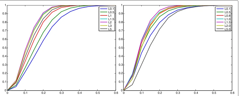
Figure 6 shows a group of p(r) for distributions distp(xS) with variouspvalues, where the x-axis repre-sents the radius r. In this experiment, the range mea-surements are corrupted by additive Gaussian noise (left graph) and Laplacian noise (right graph), respectively, with mean 0 and standard deviation 0.2. The anchor loca-tions are the same as the previous simulation, and 10,000 rounds of simulations are run to generate p(r)for eachp
value under each type of noise.
A distribution with p(r) that is close to the upper-left corner of the graph is desired, since it is spikier and demonstrates the robustness of the corresponding spring potential with respect to the specific type of noise. There-fore, as shown in Figure 6, the spring potential withp=2 works the best under Gaussian noise, while the potential withparound 1.3 performs well with Laplacian noise.
We further compare the q-quantile of the distribu-tions, to find the q-optimal Lp potential as described above, under Gaussian and Laplacian noise. The simu-lation results are shown in Figure 7, where the x-axis represents thepvalues and the y-axis shows the radius
r. The left and right hand graphs show the quantile com-parison under Gaussian and Laplacian noise respectively. The same simulation settings are used as the previous experiment, and 20%, 50%, 80%, and 90% quantiles of distributions with variouspvalues are compared.
It is easy to read the q-optimal spring potential from Figure 7. For example, p = 2 is the 90%-optimal spring potential under Gaussian noise in the group ofLp poten-tials, whilep = 1.3 is the 80%-optimal spring potential under Laplacian noise.
To conclude, the distributed spring model algorithm has the advantage that it can easily adapt to different types of noise, and the appropriate spring potential can be cho-sen according to the numerical scheme described in this section.
6 Customizing the potential for faster
convergence
In the previous section, all the potential functions that we have discussed are generic Lp norms. Different types of potential functions work for different types of noise. How-ever, in practical scenarios, situations can be more con-voluted. Searching for the optimal value ofpmay not be enough. Moreover, as the system grows large, with more sensors to localize, convergence speed becomes a more important measure of the performance of our algorithm.
6.1 Spring with “lock-in” mode
A commonly observed phenomenon in the spring model algorithm is that even when some part of the system has approximately reached the correct configuration, due to the soft spring and under-damped environment, the sys-tem continues to oscillate before eventually converging to a low-estimation-error state. This can significantly pro-long the convergence time of the system. Increasing the spring strength or the viscous coefficient of the environ-ment may not be effective either because these changes may cause the system to fall into local minima and reach premature convergence.
To cure this problem, one simple idea is to design the springs so that they can “lock in” when the actual dis-tance between two sensors is approximately the same as the length of the spring. To be more specific, we would like the strength coefficient to be significantly higher when
0 0.1 0.2 0.3 0.4 0.5 0.6
0 0.1 0.2 0.3 0.4 0.5 0.6 0.7 0.8 0.9 1
L0.1 L0.5 L1 L1.5 L2 L3 L5
0 0.1 0.2 0.3 0.4 0.5 0.6
0 0.1 0.2 0.3 0.4 0.5 0.6 0.7 0.8 0.9 1
L0.1 L0.5 L0.8 L1.0 L1.5 L2.0 L5.0
0 0.5 1 1.5 2 2.5 3 3.5 4 4.5 5 0.05
0.1 0.15 0.2 0.25 0.3 0.35 0.4
20% quantile 50% quantile 80% quantile 90% quantile
0 0.5 1 1.5 2 2.5 3 3.5 4 4.5 5 0
0.05 0.1 0.15 0.2 0.25 0.3 0.35
20% quantile 50% quantile 80% quantile 90% quantile
Figure 7Comparison of quantiles for distributions distp(xS).Comparison of quantiles for distributions distp(xS), where the x-axis represents the
pvalues and the y-axis shows the radiusrof the circle. 20%, 50%, 80%, and 90% quantiles of distributions with variouspvalues are compared. Left: quantile comparison under Gaussian noise; Right: quantile comparison under Laplacian noise.
the spring approaches its natural state. This way, in the situation where the sensors have approximately reached the correct configuration, the system will “harden-up” to keep the current configuration so as to avoid being dis-turbed into disorder again. If handled properly, the newly designed spring system can reach the correct configura-tion faster than the vanilla spring model algorithm.
This idea can be viewed from another perspective: The incremental methods [4,5] are actually the case in which all springs are rigid (with infinite strength), so that all locally resolved configurations are kept unchangeable. The concurrent method (e.g., the vanilla spring model) is another extreme in which nothing is kept fixed until the very end. This new spring model with “lock-in” mode is something in between. Specifically, we make well-configured parts of the entire system more rigid than the ill-configured parts, so that we can take potential benefits from both methods.
To make things simple and concrete, we assume the new spring to be a Hooke spring (linear force), with differ-ent strengths for differdiffer-entd = xi −xj −dij values. Fordgreater than a critical distanceρ, we assume that the spring is softer, with strength coefficientk0; and for dless thanρ, we assume that the spring is harder, with strength coefficientk1, wherek1>k0. Therefore, the force function is as shown below:
f(x)=
−k1x |x| ≤ρ
−k0x |x|> ρ
. (23)
A typical potential function for the customized spring potential is shown in Figure 8. Note that there is a “potential well” with radiusρ. Therefore, whendis no more than ρ, the two sensors will be locked in with a strong bond.
6.2 Numerical caveats
Ideally, the “lock-in” mode strength coefficientk1should be very high compared to the normal strength so that the length is effectively fixed. However, since we need to evolve the spring model numerically with a fixed time stept, a very high spring strength can result in unstable numerical results. Therefore, in our simulation, the lock-in mode sprlock-ing strength is chosen to be 3 to 5 times that of the normal spring strength. Despite the moderatek1value, the customized spring potential is proven to be effective by the simulation result next.
0 100 200 300 400 500 600 700 800 900 1000 10−2
10−1
100
Hooke force with soft spring Hooke force with strong spring Spring with Lock−in Mode
0 100 200 300 400 500 600 700 800 900 1000 10−3
10−2
10−1 100
Hooke force with soft spring Hooke force with strong spring Spring with Lock−in Mode
Figure 9Comparison of convergence rates.Left: range measurements with no noise; Right: range measurements corrupted with Gaussian noise with zero mean andσ=0.1.
Meanwhile, the choice of variable ρ is also essential to fully exploit the benefits of the customized spring potential. Too small values ofρhave almost no effect on improving the computational efficiency, since it is rather difficult for the springs to fall into the very narrow “lock-up” mode. Too largeρleads to premature lock up of too many springs, which forces the system into an undesirable local minimum. In practice, the rule of thumb is to select ρto be of similar magnitude as the noise level.
6.3 Simulation results
To demonstrate the efficacy of the spring model algorithm with “lock-in” mode, we compare the convergence speed of the following three cases:
1. Hooke spring with soft strengthk0;
2. Hooke spring with hard strengthk1;
3. Customized spring potential withk1withinρandk0
beyond that range.
It is worth noting that dimension expansion is applied in all three cases.
The setup with long-range anchors discussed in Section 3 (shown in Figure 1) is employed, which includes 800 normal sensors with communication radius 0.1, and four anchors with broadcast radius 1
2√2. We choose vis-cosityβ=1, critical radiusρ=0.05, andk1=5k0=250. The aforementioned three cases are compared under two scenarios: range measurements with no noises and range measurements corrupted by additive Gaussian noise with mean 0 and standard deviation 0.1.
Figure 9 illustrates the comparison for one particular run of the three cases. It is clear from the figure that the customized spring case converges at a much faster rate, with or without noise. In both situations, the case with customized spring potential reaches the same level of estimation error with about 150 fewer iterations than its counterparts.
Table 1 Comparison of average convergence rates under different noise levels
Noise level Spring type Error rate at iterations of multiples of 100
σ =0.00 Soft spring 0.2467 0.1468 0.1514 0.1402 0.0702 0.0419 0.0256 0.0174
Strong spring 0.2501 0.1568 0.1796 0.1077 0.0750 0.0437 0.0277 0.0189
“Lock-in” mode 0.1347 0.1651 0.1013 0.0527 0.0325 0.0213 0.0144 0.0100
σ =0.05 Soft spring 0.2486 0.1458 0.1499 0.1406 0.0693 0.0419 0.0259 0.0181
Strong spring 0.2508 0.1566 0.1784 0.1085 0.0745 0.0437 0.0285 0.0190
“Lock-in” mode 0.1340 0.1651 0.1004 0.0519 0.0323 0.0216 0.0151 0.0128
σ =0.10 Soft spring 0.2485 0.1478 0.1528 0.1389 0.0710 0.0427 0.0270 0.0204
Strong spring 0.2507 0.1569 0.1791 0.1082 0.0742 0.0438 0.0288 0.0215
“Lock-in” mode 0.1363 0.1640 0.1016 0.0528 0.0334 0.0236 0.0199 0.0214
0 0.02 0.04 0.06 0.08 0.1 0.12
Integrated Localization Error
Hooke force with soft spring Hooke force with strong spring Spring with Lock−in Mode
σ = 0 σ = 0.05 σ = 0.1
Figure 10Comparison of integrated convergence rates.Comparison of integrated convergence rate under Gaussian noise with standard deviation 0.00, 0.05, and 0.10.
More detailed simulation results are shown in Table 1, which records the average error rate of 100 independent simulations, at iterations of multiples of 100. The results in Table 1 demonstrate that the algorithm with customized spring potential works consistently better than the other two cases.
Note that there are rises and falls in the aggregated local-ization error in Table 1, because of the oscillations in the spring model. To better quantify the difference in con-vergence speed, we compute the integrated localization error of the entire process of the algorithm, i.e., the ratio between the total area under the convergence curve and the total number of iterations (800 in this experiment), and depict the results in Figure 10. It is obvious that under different noise levels, the customized spring model out-performs the other two cases significantly. The average localization error throughout the process of convergence is merely about 60% of those of its counterparts.
It is worth mentioning that both extreme cases, with soft and strong springs, underperform the customized spring case, which is a compromise of two types of springs. It is the combination of the two that creates effective improve-ment in convergence speed, without compromising the final localization error.
7 Conclusion
In this article, we have discussed several techniques to improve a spring-model-based algorithm that solves sen-sor localization problems in a fully distributed manner. Our prototype algorithm, with no prior knowledge of the coordinates of the sensors except a few anchor points, iteratively localizes the sensors using only short-range communication among neighboring sensors.
The first technique to improve the prototype algorithm is based on expanding a two-dimension problem into three dimensions. The dimension expansion technique can greatly reduce the occurrence of the “folding” phe-nomenon and hence prevent the algorithm from falling into local minima.
Second, we have investigated the optimality of different types of spring potential functions under different types of noise. Using a simplified model, our simulation demon-strates that Lp potential works best for Gaussian noise
when p ≈ 2, whilep ≈ 1.3 works best for Laplacian
noise. This simulation based conclusion sheds some light on spring-model selection under different noise circum-stances.
Third, we have discussed the customized design of a spring model beyond Lp potential functions to acceler-ate convergence speed. The customized spring model has higher strength when the distance between sensors is close to the true length of the spring. Extensive simula-tions demonstrate that this customized spring model can effectively “lock in” correctly localized sensors and hence make the iterative algorithm more efficient. From another perspective, this customized spring model can be deemed to be a compromise between incremental and concurrent sensor localization algorithms.
Competing interests
The authors declare that they have no competing interests.
Acknowledgements
Advances in Multi-Sensor Adaptive Processing (CAMSAP), San Juan, Puerto Rico, December 2011.
Received: 11 May 2012 Accepted: 4 January 2013 Published: 15 February 2013
References
1. F Franceschini, M Galetto, DA Maisano, L Mastrogiacomo, A review of localization algorithms for distributed wireless sensor networks in manufacturing. Int. J. Comput. Integrat. Manufactur.22(7), 698–716 (2009) 2. N Patwari, J Ash, S Kyperountas, IAO Hero, R Moses, N Correal, Locating
the nodes: cooperative localization in wireless sensor networks. IEEE Signal Process. Mag.22(4), 54–69 (2005)
3. K Langendoen, N Reijers, Distributed localization in wireless sensor networks: a quantitative comparison. Comput. Netw.43(4), 499–518 (2003). [http://dx.doi.org/10.1016/S1389-1286(03)00356-6]
4. C Savarese, JM Rabaey, K Langendoen, inProceedings of the General Track of the USENIX Annual Technical Conference,ATEC ’02. Robust positioning algorithms for distributed ad-hoc wireless sensor networks (USENIX Association, Berkeley, CA, USA, 2002), pp. 317–327
5. D Moore, J Leonard, D Rus, S Teller, inProceedings of the 2nd International Conference on Embedded Networked Sensor SystemsSenSys ’04. Robust distributed network localization with noisy range measurements (ACM, New York, 2004), pp. 50–61
6. AT Ihler, IJW Fisher, RL Moses, AS Willsky, Nonparametric belief propagation for self-localization of sensor networks. IEEE J. Sel. Areas Commun.23(4), 809–819 (2005)
7. H Wymeersch, J Lien, M Win, Cooperative localization in wireless networks. Proc. IEEE.97(2), 427–450 (2009)
8. X Nguyen, MI Jordan, B Sinopoli, A kernel-based learning approach to ad hoc sensor network localization. ACM Trans. Sen. Netw.1, 134–152 (2005). [http://doi.acm.org/10.1145/1077391.1077397]
9. D Tran, T Nguyen, Localization in wireless sensor networks based on support vector machines. IEEE Trans. Parallel Distrib. Syst.19(7), 981–994 (2008)
10. D Dardari, A Conti, U Ferner, A Giorgetti, M Win, Ranging with ultrawide bandwidth signals in multipath environments. Proc. IEEE.97(2), 404–426 (2009)
11. K Chintalapudi, A Dhariwal, R Govindan, G Sukhatme, inProceedings of INFOCOM 2004. Twenty-third Annual Joint Conference of the IEEE Computer and Communications Societies, vol. 4. Ad-hoc localization using ranging and sectoring, Hong Kong, 2004), pp. 2662–2672
12. Y Shang, W Ruml, Y Zhang, MPJ Fromherz, inProceedings of the 4th ACM International Symposium on Mobile Ad Hoc Networking & Computing, MobiHoc’03. Localization from mere connectivity (ACM, New York, 2003), pp. 201–212. [http://doi.acm.org/10.1145/778415.778439]
13. A Baggio, K Langendoen, Monte Carlo localization for mobile wireless sensor networks. Ad Hoc Netw.6(5), 718–733 (2008). [http://dx.doi.org/ 10.1016/j.adhoc.2007.06.004]
14. J Liu, Y Zhang, F Zhao, inProceedings of the 7th ACM International Symposium on Mobile Ad Hoc Networking and Computing, MobiHoc’06. Robust distributed node localization with error management (ACM, New York, 2006), pp. 250–261. [http://doi.acm.org/10.1145/1132905.1132933] 15. Y Shen, M Win, Fundamental limits of wideband localization–Part I: a
general framework. IEEE Trans. Inf. Theory.56(10), 4956–4980 (2010) 16. Y Shen, H Wymeersch, M Win, Fundamental limits of wideband
localization–Part II: cooperative networks. IEEE Trans. Inf. Theory.56(10), 4981–5000 (2010)
17. NB Priyantha, H Balakrishnan, E Demaine, S Teller, inProceedings of the 1st International Conference on Embedded Networked Sensor Systems,
SenSys’03. Anchor-free distributed localization in sensor networks (ACM, New York, 2003), pp. 340–341
18. C Gotsman, Y Koren, inGraph Drawing, Lecture Notes in Computer Science, vol. 3383. Distributed graph layout for sensor networks (Springer Berlin/Heidelberg, 2005), pp. 273–284
doi:10.1186/1687-6180-2013-20
Cite this article as:Yuet al.:Dimension expansion and customized spring potentials for sensor localization. EURASIP Journal on Advances in Signal Processing20132013:20.
Submit your manuscript to a
journal and benefi t from:
7Convenient online submission 7Rigorous peer review
7Immediate publication on acceptance 7Open access: articles freely available online 7High visibility within the fi eld
7Retaining the copyright to your article