Volume 2008, Article ID 786431,11pages doi:10.1155/2008/786431
Research Article
The Likelihood Ratio Decision Criterion for Nuisance Attribute
Projection in GMM Speaker Verification
Boˇstjan Vesnicer and France Miheliˇc
Faculty of Electrical Engineering, University of Ljubljana, Trzaska 25, 1000 Ljubljana, Slovenia Correspondence should be addressed to Boˇstjan Vesnicer,[email protected] Received 19 November 2007; Revised 26 March 2008; Accepted 25 June 2008
Recommended by Søren Jensen
We propose a way of integrating likelihood ratio (LR) decision criterion with nuisance attribute projection (NAP) for Gaussian mixture model- (GMM-) based speaker verification. The experiments on the core test of the NIST speaker recognition evaluation (SRE) 2005 data show that the performance of the proposed approach is comparable to that of the standard approach of NAP which uses support vector machines (SVMs) as a decision criterion. Furthermore, we demonstrate that the two criteria provide complementary information that can significantly improve the verification performance if a score-level fusion of both approaches is carried out.
Copyright © 2008 B. Vesnicer and F. Miheliˇc. This is an open access article distributed under the Creative Commons Attribution License, which permits unrestricted use, distribution, and reproduction in any medium, provided the original work is properly cited.
1. INTRODUCTION
The basic problem in speaker recognition can be formulated like this. Given two speech recordings, decide whether they belong to the same speaker or they belong to two different speakers. Putting it another way, our task is to decide whether the differences between the recordings (i.e., the intersession variability) are better attributable to the interspeaker variability or to the intraspeaker variability. Intraspeaker variability refers to all the phenomena that cause different recordings of the same speaker to sound different from each other. Usually this can be attributed mostly to channel effects, although some other factors (e.g., the aging phenomenon, the state of health and mind as well as text dependency) can play an important role.
The problem of channel variability is especially appar-ent during telephone speech, where there are differappar-ent transmission channels and different handset types involved. Performance degradation due to channel variability has been clearly demonstrated during a few previous NIST speaker recognition evaluations [1].
Many methods have been proposed to tackle the problem of channel variability. Based on their application domain, they can be categorized into three groups: feature-domain [2–5], model-domain [6–9], and score-domain [10, 11].
Since no individual method is capable of completely remov-ing the channel effects, it is common practice to combine a number of different methods together.
Recently, eigenchannel analysis (or its more advanced counterpart, joint factor analysis) and nuisance attribute projection (NAP) have become especially popular among the model-based methods [12–15]. The main reason for their widespread adoption is that they are both unsupervised and they treat channel effects as continuous rather then discrete and thus do not require a special preprocessing step for channel detection, which is the case for other methods.
Although the key algorithm of both methods is formu-lated as an eigenvalue problem, their implementation and usage differ significantly. While the first one was designed to be used in combination with a decision criterion based on the likelihood ratio (LR) statistics, the other was originally designed to work with a criterion based on the support vector machines (SVMs). In this work, we point out that there is no real reason for such a distinction, since both methods can be used with both LR-based and SVM-based decision criteria. To prove our case, we propose three different variants of integrating the NAP approach with the LR-based decision criterion.
Using the NIST 2005 data set, we compare the performance of discriminative (SVM-based) and generative (LR-based) decision criteria in combination with NAP-based channel variability compensation. We found that both criteria exhibit comparable performance, and more importantly that the overall performance can be further improved if we carry out the score-level fusion of both approaches.
The remainder of this paper is organized as follows. In Section 2, a brief introduction to GMM-based speaker verification is presented. InSection 3, a short review of NAP-based session variability modeling is given. InSection 4, the LR and SVM decision criteria are presented, and we describe how they give rise to different implementations of NAP. In
Section 5, experimental results on the core test of the NIST SRE 2005 [16] are presented and analyzed. In the last section, conclusions are given and directions for further research are suggested.
2. GMM-BASED SPEAKER VERIFICATION
Although there has recently been some success reported with methods for text-independent speaker recognition that try to exploit the high-level information (e.g., prosody) embraced in the speech signal, their performance is still inferior to that of the methods which are based on the low-level acoustic properties of the speech signal [17–19]. Most of these acoustic-based methods that perform well are based on Gaussian mixture modeling (GMM) of the cepstral features. Here, we will give a brief overview of the main steps involved in GMM-based speaker verification.
The main assumption in GMM-based speaker verifica-tion is that each speaker can be represented as a weighted sum (mixture) ofKmultivariate diagonal covariance Gaus-sian densities, defined over a D-dimensional feature space (The number of Gaussians is typically 512 or 2048.):
p(x)=
K
k=1
πkN
x|µk,Σk
. (1)
Since only a limited amount of the target speaker’s data is available in practice, the maximum likelihood (ML) estimation of the parameters of the speaker model would lead to overfitting. A better way would be to use a speaker-independent GMM—usually referred as a universal back-ground model(UBM)—and estimate the parameters of the target speaker model by means of maximum a posteriori
(MAP) adaptation [20].
Although, in general, all the parameters (i.e., weights, mean vectors, and covariance matrices) could be adapted, experiments show that it is better to adapt only the mean vectors, while keeping the weights and covariance matrices constant [21].
An important consequence of the UBM approach is that it induces a strict ordering of the Gaussian mixture compo-nents in the speaker models. This allows us to concatenate the components’ mean vectors into one composite vector—
supervector.
3. NUISANCE ATTRIBUTE PROJECTION APPROACH TO SESSION VARIABILITY COMPENSATION
3.1. Relevance maximum a posteriori
In order to explain the NAP approach to session variability compensation, it is worthwhile to look first at the MAP algo-rithm, which is used for deriving the speaker models from the UBM. Since we are not adapting weights and covariance matrices, it is sufficient to specify a prior distribution only for the mean vectors, which takes the following form:
mk(s)=mk+dkzk(s), k=1,. . .,K, (2)
wheremk is a speaker-independent mean vector of thekth
mixture component, dk is a D×D diagonal matrix, and
zk(s) is a speaker-dependent random vector with a standard
normal distribution, which implies thatmk(s) is distributed
normally with a meanmkand a diagonal covarianced2k.
Given the training dataX(s)= {x1(s),. . .,xT(s)}for the
target speakers, we are able to derive a MAP estimate of the vectormk(s), which is given by
Emk(s)
=mk+
I+d2kΣ−k1Nk
−1
d2kΣ−k1
Fk−Nkmk
, (3)
where the statisticsNkandFkare computed in the E-step of
the EM algorithm using the following relations:
Nk= T
t=1
γk,t,
Fk= T
t=1
γk,txt(s),
(4)
whereγk,tis the responsibility of the mixture componentk
for generating the observationxt(s).
Although matrixdkcan be estimated from the data [22]
itself, it is usually assumed to be related toΣ−1
k by an equation
of the form d2
k = τ−1Σk. The constant τ is known as a
relevance factor and is chosen empirically, typically in the range between 8 and 16 [21].
The MAP estimate of the vectors mk(s) should ideally
be identical (or sufficiently similar at least) for different recordings of the same speaker. Unfortunately, this is not the case, since we know that different channels cause the same speaker to sound different from one recording to another. Nevertheless, it turns out that it is possible to compensate (to some extent) for the channel effects if we make some minor assumptions about the channel.
3.2. Nuisance attribute projection
The problem that we want to address is, how to decompose, for a given recording, the speaker- and channel-dependent supervectorM, obtained by a MAP adaptation of the UBM (3), to the speaker-dependent supervectorSand the channel-dependent supervectorC:
where the offsetM0corresponds to the supervector
represen-tation of the UBM.
The linear model of (5) states that perturbations of the background model can be split linearly into a speaker-dependent and a channel-speaker-dependent parts. Although this linear assumption plays the central role in most well-performing models of channel variability [5,7, 9,14], an explicit evidence for its validity has not yet been presented.
In order to present the arguments for the linearity in (5), it helps to consider the channel effects as noise, which is being convolutionally mixed with speech in the signal domain. Since convolution in the signal domain becomes addition in the cepstrum domain, the cepstral feature vectors consist of a sum of speech and noise (channel). If we further treat speech and channel as two independent random variables, each of them being distributed according to a (finite) mixture of Gaussians (MoGs), it follows (see the appendix) that their sum is also distributed as a MoG. Moreover, each mean of this MoG equals the sum of two means, one coming from the speech MoG and the other from the channel MoG.
Note, however, that although the number of Gaussian components in the sum will be M·N, where M and N are numbers of components of the speech and channel GMM’s, respectively, not all of the components will be observed—due to a finite duration—for a specific recording. Fortunately, this hindrance can be avoided by incorporating prior knowledge while inferring the parameters of the GMM (i.e., Bayesian learning, MAP adaptation).
To be able to carry out the decomposition, it turns out that we have to confine the channel-dependent supervector to lie in a low-dimensional subspace. This requirement seems reasonable, since the channel should not be able to transform one speaker into another, otherwise speaker recognition would be an ill-posed problem. In fact, some evidence has been presented [23] which indicates that the channel covariance matrix is indeed of low rank.
If we assume that the channel variability is constrained to a low-dimensional subspace (given by the matrix U) of a supervector space and that the channel space and speaker space intersect only at the origin, then we are able to estimate the channel componentCsimply by centering the speaker-and channel-dependent supervector M, projecting it onto the channel subspace, and finally projecting the resulting supervector from the channel subspace back to the original supervector space:
C=UU∗M−M0
. (6)
By knowing the channel C, retrieving the speaker componentSis as simple as rearranging (5).
Since they were found in the cepstral domain, the projection of supervectors can be alternatively seen as a filtering operation—so, projecting the supervector into the speaker-subspace means that certain kinds of (speaker-dependent) filtering will be allowed, while other kinds of (channel-dependent) filtering will be suppressed.
The NAP approach is illustrated inFigure 1.
C M
− M
0
S
Figure 1: Schematic illustration of the NAP technique in a
3-dimensional supervector space. The speaker- and channel-dependent supervector M can be written as the sum of two supervectors, one of which (S) lies in the speaker space and the other (C) lies in the channel space.
3.3. Channel subspace estimation
In contrast to the diagonal matrixdk, the channel subspace
matrix U has to be estimated from the data. The only requirement is that we have a sufficiently large database with multiple recordings available for each speaker. The steps needed to estimate the channel subspace matrix can be summarized with the following algorithm.
(i) For each recording, estimate a speaker- and channel-dependent supervector (see (3)).
(ii) Compute the mean supervector of each speaker by averaging the supervectors from all the recordings of that speaker. This averaging process will effectively filter out (at least if the number of recordings is sufficiently large) the channel component, since it is assumed to be zero-mean distributed.
(iii) Calculate the channel component of each recording by subtracting the corresponding mean supervector. (iv) Use the principal component analysis (PCA)
tech-nique to estimate the firstnlargest eigenvalues and the corresponding eigenvectors from the covariance matrix of the channel supervectors.
Since the dimension of the supervectors can be very large, a straightforward PCA decomposition will not work in practice. A simple solution, popularized by Turk and Pentland [24], is based on the fact that the nonzero-valued eigenvalues of the matrix productAATare the same as those
of the productATA. Yet another alternative would be to use
the probabilistic variant of the PCA algorithm [25].
3.4. Relation to joint factor analysis
out the channel component, the joint factor analysis treats the channel and speaker supervectors as hidden variables and derives a special ML algorithm to estimate the matrixU(and possibly also other hyper-parameters) from their posterior distributions (instead of point estimates).
Although joint factor analysis is evidently theoretically more advanced than NAP, its drawback is that it is compu-tationally more demanding and it is harder to implement. Since it is based on a probabilistic approach, it can only be applied to GMM-based speaker recognition. On the other hand, NAP is easier to implement and has a broader scope of applications, as demonstrated recently by the impressive per-formance of NAP in the context of the maximum likelihood linear regression (MLLR) approach to speaker recognition [14], and even in high-level speaker recognition [17].
4. DECISION CRITERIA
Many different classifiers can in principle be used for making the decision for or against the hypothesis that the speaker in the test utterance is the same as the speaker in the training utterance. However, the most common and successful for speaker verification have been LR and SVMs, which will be presented in the following subsections. Note that only the basic concepts of SVMs will be described; for a more general treatment see [26].
4.1. The LR-based decision criterion
If the decision criterion is based on the likelihood ratio, then the verification score is calculated as (In practice, the likelihood ratio is computed in the log domain for numer-ical reasons. Moreover, the score should be appropriately normalized to compensate for the different lengthsTof the feature vector sequences.)
pX|Λs
pX|Λ0
, (7)
whereXis a feature vector sequence of lengthT, representing the test utterance, whileΛsand Λ0 denote the parameters
(weights, mean vectors, and covariance matrices) of the speaker model (estimated from the training utterance) and UBM, respectively.
4.2. The SVM-based decision criterion
An SVM is a two-class classifier, based on the concept of the maximum margin. It can be expressed as a separating hyperplane given by
f(x)=
N
i=1
αiyiK
x,xi
+b, (8)
within the constraintsNi=1αiyi = 0 andαi > 0. Theyiare
target values (either−1 or 1, depending on which class the corresponding support vectorxicomes from). The function
Kis called the kernel, and it has to obey Mercer’s condition. A class decision for vectorx is based on whether the value
f(x) is above or below a given threshold.
Although SVMs were originally applicable only to fixed-length data (i.e., vectors), they were later extended to work also with variable-length data in a straightforward way through the use of sequence kernels. The sequence kernel can be defined as
K(X,Y)=Φ(X)∗R−1Φ(Y), (9)
whereΦ(X) andΦ(Y) are high-dimensional vector represen-tations of the sequencesX and Y, respectively, andR is a diagonal matrix. Note that the “kernel trick” is redundant, since the sequence expansion is done explicitly. Moreover, if each vector Φ(X) is multiplied by R−1/2, a linear SVM
is obtained. As a consequence, an SVM model can be represented in a compact form [27], which enables a rapid evaluation of the value f(X).
Two popular sequence kernels for speaker verification are the generalized linear discriminant sequence kernel [27] and the GMM supervector kernel [28]. We will focus on the latter. The GMM training described in the previous section can be seen as an expansion of a sequence of cepstral vectors into a GMM. A natural choice for a distance between GMMs would be the Kullback-Leibler (KL) divergence. Unfortunately, the KL divergence does not obey the Mercer’s condition and there exists no closed-form solution for calculating the KL divergence between GMMs. So instead of using the KL divergence directly, we consider its upper bound [29], which satisfies the Mercer’s condition. The diagonal entries of the matrixR−1 are, in this case, given byπ
kΣ−k1,
whereπk are the mixture weights andΣkare the covariance
matrices of the UBM.
4.3. Combining NAP with LR and SVMs
While there have been different variants of LR-based classi-fication strategies proposed, which naturally arise from the joint factor analysis model [23] for speaker verification, the NAP approach has been limited to the SVM-based decision criterion [9,30]. The reason for this discrepancy comes from the fact that the LR criterion is asymmetric in the sense that only the training utterance is used to estimate the speaker model (supervector), while the SVM criterion is symmetric since both the training and the test utterance are “expanded” to supervectors.
We see that NAP suits well the SVM criterion, since both the training and the test supervectors can be compensated in the same way by simply projecting out the channel component of each supervector (see (7)).
4.3.1. Feature space channel compensation
The solution of transforming features to compensate for the channel mismatch between the training and test utterances (in the context of GMM-based speaker recognition) became known as feature mapping [5]. Recently, a very similar approach has been proposed by Castaldo et al. [15] for the eigenchannels, which can be adapted to the NAP approach in a straightforward way.
In the first step, the channel component C of the utterance is detected by projecting the centered supervector Mto the channel subspace (see (6)). In the second step, this channel supervector is used to transform each feature vector xtusing the following formula:
xt=xt−
K
k=1
γk,tck, (10)
whereγk,tis the posterior probability (responsibility) that the
observationxtwas generated by thekth mixture component
andckis part of the supervectorCthat corresponds to the
kth mixture component.
In this way, we are able to compensate for both the training and test utterances prior to training the target speaker model and calculating the LR score.
An important property of the feature space channel compensation is that it can be regarded as a (front-end) preprocessing step and is therefore independent of the application and the classifier. For example, a similar feature space compensation method was recently used in a speech recognition task [31].
4.3.2. Asymmetric channel compensation
Another possibility is to normalize the training utterance in the same way as in the SVM case, and to normalize the test utterance in the feature space. A similar strategy was proposed recently for the eigenchannel approach [13].
4.3.3. Model space channel compensation
We propose another alternative where both the training and test utterances are normalized in the model space. The idea is to transform the channel component of the training supervector M from the training channel C to the test channelCt, using the following equation:
M=M−C−Ct
=M0+S+Ct. (11)
The resulting supervectorMis converted back to GMM space and then used for calculating the nominator of the LR (see (8)).
Since the UBM, which is used for calculating the denom-inator of the LR, is inherently channel-neutral, (The channel component has been averaged out in the training process because the UBM is trained from a large number of different speakers recorded in many different channel conditions.) it is important to adapt the UBM in a similar fashion in order to avoid any bias towards positive LR scores. Note, however, that the normalization of the UBM is not necessary when a t-norm score t-normalization is applied, since the denominator of (7), in this case, effectively drops out.
Observe that only the speaker component of the training signal is required, while the channel component is discarded. On the other hand, the speaker component of the test signal is discarded, while the channel component is needed to adapt the training speaker supervector to the test conditions. Since this is very similar to the idea of the standard eigenchannel approach and is also more straightforward to implement than the other two alternatives, we have decided to use the model-space variant of the channel compensation algorithm in our experiments.
5. EXPERIMENTS
We carried out the verification experiments on the core condition (1conv4w-1conv4w) of the NIST 2005 speaker recognition evaluation (SRE) [16]. This evaluation set consists of 636 target speakers (372 females, 264 males) and 31418 test trials (2771 target trials, 28647 impostor trials). For each target speaker, there is a 5-minute-long recording available, containing roughly 2 minutes of speech. Note that in order to obey the rules of the NIST protocol, each trial must be processed independently of all the others.
5.1. System configuration
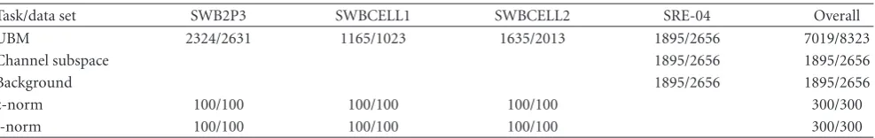
We used a (gender-dependent) UBM that contained 512 Gaussians, trained on the data collected from different data sets (Switchboard-II Phase 3, Switchboard Cellular I, Switch-board Cellular II, NIST SRE 2004, and NIST SRE 2005). The amount of data used from the individual databases is summarized inTable 1. The features were standard MFCCs (12 + log-energy, appended with their deltas), extracted every 10 milliseconds from a 25-millisecond-long windowed speech signal, using the HTK toolkit [32]. Feature warping [2] with a 3-second-long sliding window was also applied, as suggested in [7], where a strong synergy between feature warping and channel compensation was reported, although a mean-variance normalization would probably have a similar impact on the system’s performance. To remove the silence (nonspeech) frames, a simple three-Gaussians energy-based speech detector was employed [33], retaining, on average, around one-third of the frames per recording.
The channel matrixUwas estimated using the algorithm described in Section 3.3. The training data was extracted from the NIST 2004 SRE collection. It consisted of all the recordings of those speakers that were recorded in at least eight different sessions. Altogether, there were 184-female and 121-male speakers present in 4551 recordings (see
Table1: Development data sets used in the experiments. The figures in the table correspond to the number of conversation sides from the data sets that were used in different tasks.
Task/data set SWB2P3 SWBCELL1 SWBCELL2 SRE-04 Overall
UBM 2324/2631 1165/1023 1635/2013 1895/2656 7019/8323
Channel subspace 1895/2656 1895/2656
Background 1895/2656 1895/2656
z-norm 100/100 100/100 100/100 300/300
t-norm 100/100 100/100 100/100 300/300
5.2. Score normalization
The main idea of many score-normalization methods (see [10] for an overview) is to linearly transform each score s (produced by comparing the client model with the test recording) according to the following equation:
sn=
s−μ
σ , (12)
where the parametersμandσ can be estimated either from the client model (z-norm) or the test recording (t-norm).
Since both techniques can be easily combined by suc-cessively applying z-norm and t-norm (in that order), we considered also zt-norm in our experiments.
5.3. Performance metrics
Speaker-verification systems are susceptible to two type of errors—rejection of the true speaker (false rejection; miss) and acceptance of the impostor speaker (false acceptance; false alarm). The two errors are coupled in a way such that if one wants to achieve low false rejection rate, this inevitably increases the false acceptance rate (and vice versa). To see the relation between the two errors explicitly, we usually draw either receiver operating characteristic (ROC) curve or its variant, detection error tradeoff(DET) curve [34].
Accuracy of speaker-verification systems is usually mea-sured in terms of equal error rate (EER), which is the point on the DET curve where the two errors are equal. An additional performance metric, preferred by NIST, is detection cost function (DCF), which is the (minimal) weighted sum of the two errors [16].
5.4. Results and analysis
We present the results for the core condition (all trials) of the NIST SRE 2005 for the “uncompensated” baseline system and for the system where NAP-based channel compensation was performed. Two different decision criteria (SVM-based and LR-based) were applied to each of the systems. While the standard (symmetric) NAP algorithm was used for the channel compensation of the SVM-based system, the model-space variant (Section 4.3.3) of the NAP algorithm was used in the case of LR-based system. The reasons for choosing the latter are discussed in the last paragraph ofSection 4.3.3.
The impact of the channel compensation on the two-decision criteria was analyzed, and the effect of different types of score normalization (namely, z-norm, t-norm, and zt-norm) on systems’ performance was compared.
5.4.1. Effect of score normalization
The most evident observation from the DET curves in Figures 2 and 3 is that score normalization rotates the DET curve counterclockwise. This effectively means that normalization is always beneficial for the DCF point, but it can be detrimental for the EER point. However, the rotation is more evident for the LR-based systems, especially if they are combined with channel compensation (seeFigure 3(b)). This could lead to the conclusion that channel normalization tends to produce scores that are more diverse (comparing to the scores produced by systems that do not use channel normalization). This agrees with the findings presented in [7], where a similar synergy between the joint factor analysis and the zt-norm was observed.
On the other hand, the different sensitivity to score-normalization for LR- and SVM-based systems (compare Figures3(a)and3(b)) could be explained by hypothesizing that the SVMs are inherently capable of performing score-normalization to some degree already by themselves.
5.4.2. Effect of channel compensation
By comparing the performance of the BAS (see Figure 2,
0.1 0.2 0.5 1 2 5 10 20 40
M
iss
pr
obabilit
y
(%)
0.1 0.2 0.5 1 2 5 10 20 40 False alarm probability (%)
No norm z-norm t-norm
zt-norm DCF (a) BAS-SVM
0.1 0.2 0.5 1 2 5 10 20 40
M
iss
pr
obabilit
y
(%)
0.1 0.2 0.5 1 2 5 10 20 40 False alarm probability (%)
No norm z-norm t-norm
zt-norm DCF (b) BAS-LR
0.1 0.2 0.5 1 2 5 10 20 40
M
iss
pr
obabilit
y
(%)
0.1 0.2 0.5 1 2 5 10 20 40 False alarm probability (%)
BAS-SVM fusion BAS-LR fusion
BAS-SVM BAS-LR fusion DCF
(c) BAS-FUS
Figure2: Speaker verification results of the baseline (BAS) systems. The DET curves for (a) the SVM and (b) LR decision criteria as well as (c) their fusion are shown. The black circle on each DET curve represents the DCF point.
5.4.3. Fusion of LR and SVM systems
Although the idea of fusing similar classifiers into a better one is not new (see, e.g., [35]), it has not been extensively used for speaker-verification. Most of speaker-verification systems that make use of score-level fusion rely on combining scores from highly heterogeneous systems [36]. Therefor, we
found it interesting to explore to what extent can we improve the results by fusing scores that come from almost identical systems, trained on the same data, which differ only in one detail, that is, the decision criterion.
0.1 0.2 0.5 1 2 5 10 20 40
M
iss
pr
obabilit
y
(%)
0.1 0.2 0.5 1 2 5 10 20 40 False alarm probability (%)
No norm z-norm t-norm
zt-norm DCF (a) NAP-SVM
0.1 0.2 0.5 1 2 5 10 20 40
M
iss
pr
obabilit
y
(%)
0.1 0.2 0.5 1 2 5 10 20 40 False alarm probability (%)
No norm z-norm t-norm
zt-norm DCF (b) NAP-LR
0.1 0.2 0.5 1 2 5 10 20 40
M
iss
pr
obabilit
y
(%)
0.1 0.2 0.5 1 2 5 10 20 40 False alarm probability (%)
NAP-SVM fusion NAP-LR fusion
NAP-SVM NAP-LR fusion DCF
(c) NAP-FUS
Figure3: Speaker verification results of the NAP-based systems. The DET curves for (a) the SVM and (b) LR decision criteria as well as (c) their fusion are shown. The black circle on each DET curve represents the DCF point.
methods in the fusion.) We performed a weighted linear fusion using linear logistic regression [37], as implemented in the FoCal toolkit [38]. Although it can be seen (see Figures
2(c),3(c)) that the fusion of different score normalization
methods helps on its own, the results clearly show that the generative and discriminative decision criteria indeed
Table2: Speaker verification results of the baseline (BAS) systems. The EER and DCF figures for (a) the SVM and (b) LR decision criteria as well as (c) their fusion are given.
(a) BAS-SVM
Norm. type EER DCF
— 7.8 0.031
t-norm 7.5 0.029
z-norm 8.3 0.030
zt-norm 8.1 0.027
(b) BAS-LR
Norm. type EER DCF
— 9.9 0.044
t-norm 11.2 0.040
z-norm 10.4 0.043
zt-norm 12.0 0.040
(c) BAS-FUS
Fusion EER DCF
LR 10.3 0.038
SVM 8.0 0.026
LR + SVM 6.7 0.024
Table3: Speaker verification results of the NAP-based systems. The EER and DCF figures for (a) the SVM and (b) LR decision criteria as well as (c) their fusion are given.
(a) NAP-SVM
Norm. type EER DCF
— 6.7 0.025
t-norm 6.1 0.021
z-norm 6.8 0.023
zt-norm 6.1 0.021
(b) NAP-LR
Norm. type EER DCF
— 6.4 0.031
t-norm 6.8 0.029
z-norm 6.4 0.024
zt-norm 7.1 0.021
(c) NAP-FUS
Fusion EER DCF
LR 5.6 0.020
SVM 5.9 0.020
LR + SVM 4.5 0.018
6. CONCLUSION
We have proposed a novel way of integrating the NAP approach to channel compensation, which was previously limited to an SVM-based decision criterion, with a LR decision criterion for the speaker verification task.
Experimental results on the core test of the NIST 2005 SRE have shown that the performance of the proposed approach is comparable to the standard approach that uses SVM-based decision criterion. However, we have found out that both approaches respond differently to score normal-ization. It turns out that score normalization (especially zt-norm) is much more effective for LR than for SVM decision criterion. The apparent reasons for this discrepancy have been presented inSection 5.4.
The proposed approach provides an attractive alternative to the more general approach of joint factor analysis [22], which is computationally more expensive and harder to implement. Additionally, the PCA-based NAP algorithm, described in Section 3.3, can be easily substituted with some other method for subspace estimation, for example, independent component analysis (ICA), linear discriminant analysis (LDA), or even their nonlinear variants [39, 40]. However, the effectiveness of those methods is yet to be explored.
A further important contribution of this paper is that we confirmed that generative (LR) and discriminative (SVM) decision criteria introduce complementary information, which can significantly improve the performance of speaker verification by fusing the scores from both criteria.
APPENDIX
A. SUM OF TWO INDEPENDENT RANDOM VARIABLES
Lemma 1. If the p.d.f. of the multivariate random variableX
is given by fX(x)=
N
n=1σnN(x|μn,Σn), then its characteristic function equalsϕX(t)=
N
n=1σnexp(iμTnt−(1/2)tTΣnt). Proof. The characteristic function of a multivariate random variable is defined byϕX(t)=E[exp(itTX)], thus
ϕX(t)= x∈Rd
N
n=1
σnN
x|μn,Σn
expitTxdx. (A.1)
By linearity, we are allowed to change the order of summa-tion and integrasumma-tion:
ϕX(t)= N
n=1
σn x∈RdN
x|μn,Σn
expitTxdx. (A.2)
Solving the integral, we get the required result.
Theorem 1. Let X and Y be d-variate independent r.v.’s. If their p.d.f.’s are given by fX(x) =
N
n=1σnN(x|μn,Σn) and fY(y) =
M
m=1ωmN(y|νm,Ωm), respectively, then the distribution of the sumZ=X+Yis given by
fZ(z)= N
n=1
M
m=1
σnωmN
z|μn+νm,Σn+Ωm
Proof. The characteristic function of the sum of two inde-pendent (multivariate) random variables is given by the product of their characteristic functions. Therefore,
ϕZ(t)=
N
n=1
σnexp
iμT
nt−
1 2t TΣ nt · M
m=1
ωmexp
iνT
mt−
1 2t TΩ mt . (A.4)
After rearranging, we get
ϕZ(t)= N
n=1
M
m=1
σnωmexp
iμn+νm
T
t−1
2t
TΣ n+Ωm
t
.
(A.5)
By Lemma 1, this is exactly the characteristic function of fZ(z). Since for any characteristic function there is exactly
one probability distribution, the theorem is proved.
ACKNOWLEDGMENT
This work was supported in part by the Ministry of Defence and the Ministry of Higher Education, Science and Technology, under Contract no. M2-0210.
REFERENCES
[1] M. A. Przybocki, A. F. Martin, and A. N. Le, “NIST speaker recognition evaluations utilizing the mixer corpora—2004, 2005, 2006,”IEEE Transactions on Audio, Speech, and Language Processing, vol. 15, no. 7, pp. 1951–1959, 2007.
[2] J. Pelecanos and S. Sridharan, “Feature warping for robust speaker verification,” in A Speaker Odyssey: The Speaker Recognition Workshop, pp. 213–218, Crete, Greece, June 2001. [3] B. Xiang, U. V. Chaudhari, J. Navr´atil, G. N. Ramaswamy,
and R. A. Gopinath, “Short-time Gaussianization for robust speaker verification,” in Proceedings of IEEE International Conference on Acoustics, Speech and Signal Processing (ICASSP ’02), vol. 1, pp. 681–684, Orlando, Fla, USA, May 2002. [4] H. Hermansky and N. Morgan, “RASTA processing of speech,”
IEEE Transactions on Speech and Audio Processing, vol. 2, no. 4, pp. 578–589, 1994.
[5] D. A. Reynolds, “Channel robust speaker verification via fea-ture mapping,” inProceedings of IEEE International Conference on Acoustics, Speech and Signal Processing (ICASSP ’03), vol. 2, pp. 53–56, Hong Kong, April 2003.
[6] R. Teunen, B. Shahshahani, and L. Heck, “A model-based transformational approach to robust speaker recognition,” inProceedings of the 6th International Conference on Spoken Language Processing (ICSLP ’00), pp. 495–498, Beijing, China, October 2000.
[7] P. Kenny, G. Boulianne, P. Ouellet, and P. Dumouchel, “Joint factor analysis versus eigenchannels in speaker recognition,” IEEE Transactions on Audio, Speech, and Language Processing, vol. 15, no. 4, pp. 1435–1447, 2007.
[8] A. O. Hatch, S. Kajarekar, and A. Stolcke, “Within-class covari-ance normalization for SVM-based speaker recognition,” in Proceedings of the 9th International Conference on Spoken Language Processing (INTERSPEECH/ICSLP ’06), vol. 3, pp. 1471–1474, Pittsburgh, Pa, USA, September 2006.
[9] A. Solomonoff, C. Quillen, and W. M. Campbell, “Channel compensation for SVM speaker recognition,” in A Speaker Odyssey: The Speaker Recognition Workshop, pp. 41–44, Toledo, Spain, May-June 2004.
[10] F. Bimbot, J.-F. Bonastre, C. Fredouille, et al., “A tutorial on text-independent speaker verification,”EURASIP Journal on Applied Signal Processing, vol. 2004, no. 4, pp. 430–451, 2004. [11] R. Auckenthaler, M. Carey, and H. Lloyd-Thomas, “Score
nor-malization for text-independent speaker verification systems,” Digital Signal Processing, vol. 10, no. 1, pp. 42–54, 2000. [12] L. Burget, P. Matejka, P. Schwarz, O. Glembek, and J.
Cer-nocky, “Analysis of feature extraction and channel compensa-tion in a GMM speaker recognicompensa-tion system,”IEEE Transactions on Audio, Speech, and Language Processing, vol. 15, no. 7, pp. 1979–1986, 2007.
[13] B. G. B. Fauve, D. Matrouf, N. Scheffer, J.-F. Bonastre, and J. S. D. Mason, “State-of-the-art performance in text-independent speaker verification through open-source software,” IEEE Transactions on Audio, Speech, and Language Processing, vol. 15, no. 7, pp. 1960–1968, 2007.
[14] A. Stolcke, S. S. Kajarekar, L. Ferrer, and E. Shriberg, “Speaker recognition with session variability normalization based on MLLR adaptation transforms,” IEEE Transactions on Audio, Speech, and Language Processing, vol. 15, no. 7, pp. 1987–1998,, 2007.
[15] F. Castaldo, D. Colibro, E. Dalmasso, P. Laface, and C. Vair, “Compensation of nuisance factors for speaker and language recognition,” IEEE Transactions on Audio, Speech, and Language Processing, vol. 15, no. 7, pp. 1969–1978, 2007. [16] “The NIST year 2005 speaker recognition evaluation plan,”
2005,http://www.nist.gov/speech/tests/spk/2005.
[17] W. M. Campbell, J. P. Campbell, T. P. Gleason, D. A. Reynolds, and W. Shen, “Speaker verification using support vector machines and high-level features,”IEEE Transactions on Audio, Speech, and Language Processing, vol. 15, no. 7, pp. 2085–2094, 2007.
[18] E. Shriberg, L. Ferrer, S. Kajarekar, A. Venkataraman, and A. Stolcke, “Modeling prosodic feature sequences for speaker recognition,”Speech Communication, vol. 46, no. 3-4, pp. 455– 472, 2005.
[19] N. Dehak, P. Dumouchel, and P. Kenny, “Modeling prosodic features with joint factor analysis for speaker verification,” IEEE Transactions on Audio, Speech, and Language Processing, vol. 15, no. 7, pp. 2095–2103, 2007.
[20] J.-L. Gauvain and C.-H. Lee, “Maximum a posteriori esti-mation for multivariate Gaussian mixture observations of Markov chains,” IEEE Transactions on Speech and Audio Processing, vol. 2, no. 2, pp. 291–298, 1994.
[21] D. A. Reynolds, T. F. Quatieri, and R. B. Dunn, “Speaker verification using adapted Gaussian mixture models,”Digital Signal Processing, vol. 10, no. 1, pp. 19–41, 2000.
[22] P. Kenny, “Joint factor analysis of speaker and session vari-ability: theory and algorithms,” Tech. Rep. 06/08-13, CRIM, Montreal, Canada, 2005.
[23] P. Kenny, G. Boulianne, P. Ouellet, and P. Dumouchel, “Speaker and session variability in GMM-based speaker ver-ification,”IEEE Transactions on Audio, Speech, and Language Processing, vol. 15, no. 4, pp. 1448–1460, 2007.
[24] M. Turk and A. Pentland, “Eigenfaces for recognition,”Journal of Cognitive Neuroscience, vol. 3, no. 1, pp. 71–86, 1991. [25] M. E. Tipping and C. M. Bishop, “Mixtures of probabilistic
[26] C. J. C. Burges, “A tutorial on support vector machines for pattern recognition,”Data Mining and Knowledge Discovery, vol. 2, no. 2, pp. 121–167, 1998.
[27] W. M. Campbell, “Generalized linear discriminant sequence kernels for speaker recognition,” inProceedings of IEEE Inter-national Conference on Acoustics, Speech and Signal Processing (ICASSP ’02), vol. 1, pp. 161–164, Orlando, Fla, USA, May 2002.
[28] W. M. Campbell, D. E. Sturim, and D. A. Reynolds, “Support vector machines using GMM supervectors for speaker verifica-tion,”IEEE Signal Processing Letters, vol. 13, no. 5, pp. 308–311, 2006.
[29] M. N. Do, “Fast approximation of Kullback-Leibler distance for dependence trees and hidden Markov models,”IEEE Signal Processing Letters, vol. 10, no. 4, pp. 115–118, 2003.
[30] W. M. Campbell, D. E. Sturim, D. A. Reynolds, and A. Solomonoff, “SVM based speaker verification using a GMM supervector kernel and NAP variability compensation,” in Proceedings of IEEE International Conference on Acoustics, Speech and Signal Processing (ICASSP ’06), vol. 1, pp. 97–100, Toulouse, France, May 2006.
[31] P. Kenny, V. Gupta, G. Boulianne, P. Ouellet, and P. Dumouchel, “Feature normalization using smoothed mixture transformations,” inProceedings of the 9th International Con-ference on Spoken Language Processing (INTERSPEECH/ICSLP ’06), vol. 1, pp. 25–28, Pittsburgh, Pa, USA, September 2006. [32] “The hidden Markov model toolkit (HTK),” 2007,http://htk
.eng.cam.ac.uk.
[33] J.-F. Bonastre, N. Scheffer, C. Fredouille, and D. Matrouf, “NIST’04 speaker recognition evaluation campaign: new LIA speaker detection platform based on ALIZE toolkit,” in Proceedings of NIST Speaker Recognition Evaluation (SRE ’04), Toledo, Spain, June 2004.
[34] A. F. Martin, G. Doddington, T. Kamm, M. Ordowski, and M. A. Przybocki, “The DET curve in assessment of detection task performance,” inProceedings of the 5th European Conference on Speech Communication and Technology (Eurospeech ’97), vol. 4, pp. 1895–1898, Rhodes, Greece, September 1997.
[35] M. P. Perrone and L. N. Cooper, “When networks disagree: ensemble methods for hybrid neural networks,” in Neural Networks for Speech and Image Processing, R. J. Mammone, Ed., pp. 126–142, Chapman-Hall, London, UK, 1993.
[36] N. Brummer, L. Burget, J. Cernocky, et al., “Fusion of heterogeneous speaker recognition systems in the STBU submission for the NIST speaker recognition evaluation 2006,” IEEE Transactions on Audio, Speech, and Language Processing, vol. 15, no. 7, pp. 2072–2084, 2007.
[37] N. Br¨ummer and J. du Preez, “Application-independent evalu-ation of speaker detection,”Computer Speech & Language, vol. 20, no. 2-3, pp. 230–275, 2006.
[38] “Tools for fusion and calibration of automatic speaker detec-tion systems,” 2005, http://www.dsp.sun.ac.za/∼nbrummer/ focal/index.htm.
[39] B. Sch¨olkopf, A. Smola, and K.-R. M¨uller, “Kernel principal component analysis,” in Advances in Kernel Methods—SV Learning, B. Sch¨olkopf, C. J. C. Burges, and A. J. Smola, Eds., pp. 327–352, MIT Press, Cambridge, Mass, USA, 1999. [40] K.-R. M¨uller, S. Mika, G. R¨atsch, K. Tsuda, and B. Sch¨olkopf,