allocation of scarce water
A study about inter-annual and spatial dynamics
in agricultural land use and irrigation water use
under changing water availabilities around the
Orós reservoir in the Northeast of Brazil.
Spatial dynamics in allocation of
scarce water
A study about inter-annual and spatial dynamics in agricultural
land use and irrigation water use under changing water
availabilities around the Orós reservoir in the Northeast of Brazil.
By
Anne Leskens (Sept 2006)
Master thesis submitted to the Water Engineering and Management department of the University of Twente in cooperation with the International Institute for Geo-information Science and Earth Observation (ITC) in fulfillment of the requirements for the degree of Ingenieur (Master of Science) in Civil Engineering, specialization in Water Engineering and Management.
Assessment board
Chairman: Dr. M.S. Krol Daily supervisor: Ir. P.R. van Oel Daily supervisor: Ing. R.J.J. Dost (M.Sc.)
Conflicts in distribution of available water resources are common in the semi-arid Northeast of Brazil, mostly because of the scarcity of availability of water resulting from climatic conditions. Lacking knowledge about spatial dynamics of land use and its irrigation water use under changing water availabilities limits the determination of suitable solutions in finding the best way to allocate the scarce and strongly varying amount of available water.
The goal of study is to get more knowledge about the spatial dynamics of agricultural land use and irrigation water use under different situations of water availability around strategic water reservoirs in the semi-arid northeast region of Brazil. This is done by analyzing these aspects a spatial way, using GIS and Remote Sensing-techniques, for a research area around the Orós reservoir located in the Northeast of Brazil, during the dry seasons in 2000 to 2005.
Firstly a downscaling is carried out to 6 ‘areas of interest’, each mainly supplied by one source of water availability. Four aspects of water availability could be distinguished in the research area: rainfall, river discharges/reservoir releases, reservoir volumes and locally stored runoff. Each type of water availability is quantified for each area of interest. Secondly the agricultural land use, as largest water user, is determined by applying a land cover classification to satellite images of each year. Thirdly the irrigation water use of each area of interest in each dry season within the research period is estimated by using the Cropwat model, a model able to calculate crop irrigation requirements. The results of these three components are analyzed in a inter-annual way (how are the components evolving during the research period in a particular area of interest) and in a spatial way (how do the components of different areas of interest influence each other during the research period).
The analysis showed that the different types of water sources have different spatial and temporal ranges and different water availabilities. This determines the way in which agricultural water users, dependent on a certain water source, effect the water availability of other agricultural water users.
Rainfall and river discharge in the dry season are far too low to fulfill the irrigation water requirement of the areas that are connected to these water sources. Locally stored water is only local available; irrigation water use of this source does not noticeable effect downstream water availabilities. Water users around the reservoirs (upstream, edge, downstream) in the area influence each others water availability on different time scales: The relevant time scale around small reservoirs are estimated on 1-3 years and > 10 year around the largest reservoir. It is recommended to take these different time scales into account by defining water management actions.
Conflicten in het verdelen van beschikbaar water komen veel voor in het Noord-Oosten van Brazilië, voornamelijk als gevolg van schaarste in het beschikbaar water. Ontbrekende kennis over de ruimtelijke dynamiek van agrarisch landgebruik en geïrrigeerd watergebruik, onder wisselende situaties van water beschikbaarheid, limiteren het bepalen van bruikbare oplossingen om tot een goede verdeling van het sterk variende beschikbare water te komen.
Het doel van dit onderzoek is om meer inzicht te krijgen te krijgen in de ruimtelijke dynamiek van agrarische landgebruik en geïrrigeerd water gebruik onder wisselende omstandigheden van waterbeschikbaarheid rond strategische reservoirs in het semi-aride Noord-Oosten van Brazilië. Dit is gedaan door de ontwikkelingen in agrarisch landgebruik, geïrrigeerd watergebruik en water beschikbaarheid op een ruimtelijke manier te analyseren, gebruikmakend van GIS- en Remote Sensing-technieken in het gebied rond het Orós reservoir voor de droge seizoenen van 2000 tot 2005.
Zes gebieden, elke voornamelijk afhankelijk van één soort water toevoer, zijn vastgesteld. De aanwezige soorten van waterbeschikbaarheid in het gebied zijn: regenval, rivierwater, reservoir water en plaatselijk opgeslagen runoff. Elk type waterbeschikbaarheid is gekwantificeerd voor elk van de 6 gebieden.
Vervolgens is het agrarsiche landgebruik bepaald met behulp van satteliet beelden en een landgebruik classificatie techniek. De oppervlakten van gewassen die niet bepaald konden worden met behulp van deze techniek zijn verkregen uit data bestanden van locale instanties. Het geïrrigeerd watergebruik is geschat met behulp van het Cropwat model; een model dat in staat is de irrigatie water behoefte van een gewas te berekenen.
De drie bepaalde componenten zijn op een tijdelijke en een ruimtelijke schaal geanalyseerd.
Deze analyse liet zien dat de verschillende waterbronnen verschillende reikwijdtes en verschillende voorraden hebben en dat de relevante relaties tussen water gebruik en water beschikbaarheid zich op verschillend tijdschalen afspelen. Deze componenten bepalen voornamelijk het effect dat het watergebruik van watergebruikers van een bepaalde waterbron heeft op de waterbeschikbaarheid van andere gebruikers:
De waterbeschikbaarheid uit regenval en uit river afvoer in het droge seizoen kan niet aan de vraag van water voldoen. Lokaal opgeslagen runoff heeft alleen een lokale beschikbaarheid en beïnvloed daarom niet de waterbeschikbaarheid van benedenstroomse watergebruikers.
Water gebruikers rond de Reservoirs (bovenstrooms, aan de reservoirrand en benedenstrooms) in het gebied beïnvloeden elkaars water beschikbaarheid in verschillende tijdschalen: Rond de kleine reservoirs is de relevante tijdschaal geschat 1-3 jaar, rond het grootste reservoir is de relevante tijdschaal > 10 jaar. Het wordt aangeraden het water management aan te laten sluiten bij deze relevante tijdschalen.
First of all I want to express my thanks to my daily supervisor of the Water Engineering and Management department of the University of Twente: Pieter van Oel. During the whole research he helped me with al kind of comments and feedback. Together we explored the semi-arid ‘sertão’ of Brazil to retrieve as much ‘ground truth’ and information from local agencies as possible. Also outside the research work we had a very good time together, especially during the period in Brazil. In that aspect I also want to thank Marjella de Vries and Bertien Koopman for their good company in Brazil.
I would like to thank the chairman of my assessment board, Maarten Krol, for his rigorous and careful supervising.
I would like to express my gratitude to the water department of the International Institute for Geo-information Science and Earth Observation (ITC) in Enschede. They gave me the opportunity to get knowledge about GIS and Remote Sensing and they offered me a place to work during the GIS and Remote Sensing analysis. A special word of thank for my supervisors of the ITC: Remo Dost and Chris Mannaerts for helping me to solve all kind of problems during the GIS and Remote Sensing analysis and reviewing my report.
I am very grateful for the hospitality of the ‘Departamento de Engenharia Hidráulica e Ambiental’ at the Federal University of Ceará (UFC) in Fortaleza (Brazil) and especially for the help of professor José Carlos de Araújo and the daily company of Allexandre Cunha-Costa.
I am greatly indebted to the Brazilian family Cunha-Costa for the accommodations and the heartwarming hospitality and care they offered me during my stay in Brazil. They are justly ‘minha familia Brasileira’. Muito obrigado!
Finally, I extend a special note of thanks for the members of the graduation room at the University Twente for their good company during the writing of my thesis.
1 INTRODUCTION... 1
1.1 INTRODUCTION... 1
1.2 NATURAL CONDITIONS... 1
1.3 SOCIO-ECONOMIC CONDITIONS... 3
1.4 PROBLEM DEFINITION... 4
1.5 GOAL OF STUDY, RESEARCH QUESTIONS AND THESIS OUTLINE... 4
1.6 RESEARCH AREA... 5
2 THEORY AND METHODS... 7
2.1 INTRODUCTION:METHODOLOGY... 7
2.2 GEOGRAPHICAL INFORMATION SYSTEMS (GIS)... 9
2.3 IMAGE CLASSIFICATION... 9
2.4 IRRIGATION WATER USE...14
3 DATA PROCESSING...17
3.1 INTRODUCTION...17
3.2 PERIOD OF INTEREST...17
3.3 AREAS OF INTEREST...17
3.4 WATER AND LAND AVAILABILITY DATA...26
3.5 LAND USE DATA...34
3.6 IRRIGATION WATER USE...45
4 RESULTS ...47
4.1 INTRODUCTION...47
4.2 INTER-ANNUAL ANALYSIS PER AOI...47
4.3 INTER-AOI ANALYSIS...58
5 DISCUSSION...64
5.1 INTRODUCTION...64
5.2 UNCERTAINTY AND IMPACT ANALYSIS...64
6 CONCLUSIONS AND RECOMMENDATIONS...69
6.1 INTRODUCTION...69
6.2 CONCLUSIONS...69
6.3 RECOMMENDATIONS...74
GLOSSARY...76
Figure 1.1: Temporal course of the mean precipitation sum for the area of Ceará and Piauí... 2
Figure 1.2: Temporal course of the beginning, end and length of the dry period at the stationCedro, period 1921-1980... 2
Figure 1.3: Scheme of the large-scale circulation patterns over the tropical Atlantic... 3
Figure 1.4: Location of research area... 6
Figure 1.5: Research area detailed... 6
Figure 2.1: Methodology ... 7
Figure 2.2: Example of creating a new visualization... 9
Figure 2.3: Image classification methods and algorithms...10
Figure 2.4: Comparison classification algorithms for sample set of 2004_right...12
Figure 3.1: AOI’s ...18
Figure 3.2: Groundwater from wells ...18
Figure 3.3: Relative elevation perpendicular to river...19
Figure 3.4: Soil types per AOI...20
Figure 3.5: Border AOI 3 in 2005 due to relative elevation from the reservoir level of 6 m...21
Figure 3.6: Boundary of AOI 3 in 2005 at inlet point ...22
Figure 3.7: AOI 3 in each year...23
Figure 3.8: Operative rainfall stations in 2000...26
Figure 3.9: Monthly rainfall per AOI...27
Figure 3.10: Discharges...28
Figure 3.11: Relative reservoir volumes...29
Figure 3.12: Relationship ‘water level (h)’ and ‘available land’ at reservoir edge of Orós...31
Figure 3.13: Land availability due to water level Lima Campos reservoir ...32
Figure 3.14: Uncertainty of DEM; cross-section ...33
Figure 3.15: Uncertainty DEM overview...33
Figure 3.16: Cocos in AOI 6 ...38
Figure 3.17: Comparison DNOCS data and classification about bananas and paddy in AOI 6...42
Figure 3.18: Comparison seasonal classification results, seasonal Ematerce-data and annual IBGE-data of Paddy and Beans ...43
Figure 3.19: Amounts of water use per AOI per year...45
Figure 3.20: irrigation water use banana, rice and beans...46
Figure 4.1: Irrigation water use and water availability AOI 1 ...47
Figure 4.2: total effective rainfall and total irrigation water use AOI 1 ...48
Figure 4.3: Land use AOI 1 ...48
Figure 4.4: Irrigation water use and water availability AOI 2 ...49
Figure 4.5: total effective rainfall and total irrigation water use AOI2 ...50
Figure 4.6: Land use AOI 2 ...50
Figure 4.7: Irrigation water use and water availability AOI 3 ...51
Figure 4.8: Land use AOI 3 ...51
Figure 4.9: Irrigation water use and water availability AOI 4 ...52
Figure 4.10: Water sources and irr. water use AOI 4 ...53
Figure 4.11: Land use AOI 4...53
Figure 4.12: Irrigation water use and water availability AOI 5 ...54
Figure 4.13: Irr. water use at combinations of reservoir volume and tunnel release...54
Figure 4.14: Land use AOI 5...54
Figure 4.15: Water use AOI 5 vs 'tunnel flow minus release Lima Campos'...55
Figure 4.16: Irrigation water use and water availability AOI 6 ...56
Figure 4.18: Water use AOI 1 and AOI 2 ...58
Figure 4.19: Waterlevel-volume relationship Orós reservoir...59
Figure 4.20: Threshold tunnel ...59
Figure 4.21: Influence of water use AOI 3 on water level around tunnel inlet ...59
Figure 4.22: Water uses dry season of AOI 5 and 6...61
Figure 4.23: Cumulative effect of water use AOI 4,5 and 6 on reservoir volume Orós...61
Figure 4.24: Volume Orós reservoir 1986-2005...62
Figure 5.1: Research steps and accompanying uncertainties ...64
Figure 5.2: Varying border of AOI 3 in 2005 land use and irr. water use...65
Figure 5.3: Trendline 'waterlevel-available land'-relations...66
Table 1.1: Hydrological properties of Ceará ... 1
Table 2.1: Accuracies of algorithm methods for 2004_right ...11
Table 2.2: Example of a confusion matrix (2003_right)...13
Table 3.1: Water level data of DEM and COGERH (2006)...24
Table 3.2: results of error of interpolation methods rainfall...27
Table 3.3: Summary water and land availability ...34
Table 3.4: GPC’s: division ‘sample set (ss) – test set’ (ts) and total (tot), Landsat7 images ...34
Table 3.5: GPC’s: division ‘sample set (ss) – test set (ts)’ and total (tot), CBERS-2 images...35
Table 3.6: Used classification methods per image and results of accuracy assessment ...36
Table 3.7: Inter-annual consistency of coco...37
Table 3.8: Bean-pixels of 2004 crossed with classified maps of other years (AOI 6: Perímetro)...39
Table 3.9: Beans of 02/09/05 crossed with crops of 24/10/05, AOI 6: Perímetro ...40
Table 3.10: Beans of 02/09/05 crossed with crops of 29/09/2004, AOI 6: Perímetro ...40
Table 3.11: Numerical data (Cogher, 2006) of beans areas ...40
Table 3.12: Results of classification in AOI 1-5 for beans and grass as percentage of total agricultural land use ...41
Table 3.13: Comparison annual DNOCS data with classification results AOI 6: Perímetro ...41
Table 3.14:Comparison of IBGE data and classification results in the Iguatú municipality ...43
Table 3.15: Results Water use calculations...45
Table 3.16: Irrigation water use banana, rice and beans...46
Table 4.1: Summary correlations between water availability and land use and agricultural water use ...57
Table 4.2: Characteristics of water extraction from Orós reservoir by AOI 3...59
Table 4.3: Impact water use of AOI 5+6 on land availability AOI 3 ...60
Table 4.4: Cumulative effect...62
Table 5.1: Variation in proportion banana and paddy of +/-10% in an area of 1000 ha ...67
Table 5.2: Variation in proportion beans and banana under variation of +/-50% beans area...67
1
Introduction
1.1
Introduction
The semi-arid region of Brazil is a dry area which is subjected to recurrent, severe droughts. Several problems emerge as a consequence of these droughts. An important issue is the allocation of the available water in the dry periods. The subject dealt in this thesis is the strain between the availability of water and the use of this water.
In this chapter the reader will be firstly introduced to some important background factors of the problem about water allocation in dry periods. These background factors are the natural and the socio-economic conditions related to water allocation in the semi-arid area of Brazil (paragraph 1.2 and paragraph 1.3). Hereafter, the research problem will be defined in paragraph 1.4. The research problem is owned by a large area in the semi-arid region of Brazil. Because the area is too large to investigate, a relatively small, but representative, area is selected to take part in this research. This area is the direct neighborhood of the Orós reservoir in the state of Ceará. (see figure 1.5). Paragraph 1.5 will describe the research approach. This research area will be introduced in paragraph 1.6.
1.2
Natural conditions
1.2.1 Hydrological properties
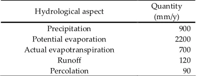
The northeast of Brazil is a semi-arid region for which precipitation is the most important climatologically variable. Recurrent droughts, “secas”, with annual rainfall totals far below average, castigate the region (Werner and Gerstengabe, 2003). For this, the region is called ´drought polygon´. Some important hydrological properties of Ceará are shown in table 1.1.
Hydrological aspect Quantity (mm/y)
Precipitation 900
Potential evaporation 2200
Actual evapotranspiration 700
Runoff 120
Percolation 90
table 1.1: Hydrological properties of Ceará (Frischkorn et al., 2003)
Also the moment of beginning and ending of the dry period, and due to that, the length of the dry period in each year is uncertain (see figure 1.2).
figure 1.1: Temporal course of the mean precipitation sum for the area of Ceará and Piauí (Werner and Gerstengarbe, 2003)
figure 1.2: Temporal course of the beginning (dotted), end (dashed) and length (solid) of the dry period at the station Cedro, period 1921-1980 (Werner and Gerstengarbe, 2003)
There is not only a temporal variation in precipitation, also a spatial distribution occur. Precipitation is distinctly decreasing from the coast to the interior of the country, with an average rainfall of approximately 2000 mm per year along the coastline and approximately 500 mm in the interior (Werner and Gerstengarbe, 2003). The conclusion of what is written above is that precipitation shows a high temporal irregularity in each particular year and a high inter-annual irregularity. Also a high spatial irregularity can be concluded.
1.2.2 Climate
The irregularity of the temporal precipitation and the recurrent droughts are caused by the climatologically properties of the area. The area is defined by a ‘trade wind region with the summery maritime weather of the trade wind limit’. This climate is most importantly characterized by a long winter period with little precipitation. The annual cycle of rainy and drought periods is controlled by large-scale circulations. The two seasons, dry and wet, are determined by the position of the Inter Tropical Convergence Zone (ITCZ): “Between 30°N and 30°S latitude, the solar energy, which is higher around the equator than in surrounding areas, is transported by a relatively simple overturning circulation, with rising motion near the equator, poleward motion near the tropopause, sinking motion in the subtropics, and an equatorward return flow near the surface. The region in which the equatorward moving surface flows converge and rise is known as the ITCZ, a high-precipitation band of thunderstorms”. The positions of high-pressure areas influence the position of the ITCZ. This high-pressure areas depend on the present sea surface temperature (SST) (see figure 1.3). If, for example, the ITCZ does not shift far enough to the south in one year due to these conditions, this can lead to a weakening of the rain period that can cause a drought (Werner and Gerstengabe, 2003)
figure 1.3: Scheme of the large-scale circulation patterns over the tropical Atlantic (Werner and Gerstengarbe, 2003)
1.2.3 Water resources Surface water
In the state of Ceará all rivers are naturally intermittent due to highly seasonally irregular precipitation rates, high evaporation rates and shallow soils on top of the crystalline basement (a basement of rock made up of minerals in a clearly crystalline state). Due to water scarcity in rivers in the dry season and to the low groundwater reserves, the only way to have water available with reasonable confidence for social and economical use is to store the excess of water during the rainy season. This policy, historically known as the ‘hydraulic approach’, directs all efforts towards the construction of artificial reservoirs (Frischkorn et al., 2003).
Groundwater
As mentioned above, the groundwater reserves in the northeast, and thus in Ceará, are low, due to the shallow soils on top of the crystalline basement. Studies about runoff reached the conclusion that, in the crystalline areas of the Semi-Arid zone an average of only 6 to 8% of the rainfall actually flows superficially or feeds aquifers by percolation. The remaining 92 to 94 % are retained by the soil or lost by evaporation or evapotranspiration (DNOCS, 1982). Around 75% of the area of Ceara contains a crystalline basement. The remaining 25% contains sedimentary water basins. These area’s with groundwater resources are located at the borders of the state. (Frischkorn, Araújo and Santiago, 2003). Even though the groundwater reserves are small compared to surface water availability, they are crucial for many cities and irrigated areas, sometimes constituting the only water source. Despite this resource’s importance, there is still little knowledge of the real availability and utilization of groundwater in the whole basin (Johnsson, 2004) (DNOCS, 1982). During the field visit in the Iguatú municipality in the state of Ceará, agricultural areas supplied by water form wells and natural lakes, were seen. This will be discussed later in chapter 3.
1.3
Socio-economic conditions
recurrent droughts were treated as essentially a supply problem. This was resolved by massive construction of reservoirs and related water infrastructure. Water reform has introduced new practices aimed at complementing this supply-side approach with demand management” (Johnsson and Kemper, 2005). “This demand management is characterized by a combination of organized public organizations, private entities and civil society representatives which make the implementation of the water resources management instruments possible, in accordance with principles established in law. The river basin committees, for example, bring stakeholders together for debates and decisions regarding problems in the watershed. Among these stakeholders are public organizations such as state secretariats and local government representatives, as well as private and state-owned water users and NGO’s. The composition of the board of directors of the Water Agencies is also a mixture of all the previous representatives” (Garrido, 2001).
1.4
Problem definition
Despite recent efforts by Ceara’s government to promote more efficient water management, the relationship between water availability and water demand is still unbalanced (COGERH and Engesoft, 1999) (Johnsson and Kemper, 2005).
Conflicts about the distribution of the available water resources are common, mostly because of the strong variation of the availability resulting from climatic conditions. Most frequent conflicts arise between the users that depend directly on reservoir water and those located further downstream and among users in the valleys rendered perennial through regulations (Johnsson, 2004). A proposition is made that the conflicts, which are reemerging in every negotiation, are related to the geographical locations of different irrigation water users around the reservoirs (Van Oel, 2006). Knowledge about this spatial dynamics of land use and its irrigation water use under changing water availabilities is limited. It is expected that better insight in this topic will give more understanding in problems of water allocation and how they can be solved. Therefore, the problem that thesis is dealing with is:
The lacking knowledge about spatial dynamics of land use and its irrigation water use under changing water availabilities.
1.5
Goal of study, research questions and thesis outline
Goal of study
The goal of this study is to explain the inter annual spatial dynamics of land use and irrigation water use under different conditions of water availability around strategic water reservoirs in the semi-arid northeast region of Brazil, by analyzing changes in land use, irrigation water use and water availability in a spatial way for the period from 2000 until 2005 in a representative area.
Demarcation
this area is the availability of satellite images and hydrological data. A further description of this area will be given in paragraph 1.6.
The research period includes the dry season of 2000 to 2005. This temporal demarcation will be explained in paragraph 3.2. Only agricultural land uses supplied by irrigation water will be examined, because these land uses have the highest water demand in the basin during the dry periods.
Research questions
1. What is the annual amount of available water for irrigation in the dry season and which areas have access to it?
2. How much land do the different irrigated agricultural land uses cover in the dry season and what is their spatial distribution?
3. What are the amounts of irrigation water use, related to land use, in the dry season? 4. How are water availability, agricultural land use and irrigation water use related
between 2000 and 2005 in different focus areas in the research area?
5. How are spatially explicit water availability, agricultural land use and irrigation water use of different focus areas mutually related in the research area between 2000 and 2005.
Structure of thesis
The methods and theories to answer the research questions will be discussed in chapter 2. The results of research questions 1, 2 and 3 will be dealt in chapter 3: ‘Data processing’. Research questions 4 and 5 will be dealt in chapter 4: ‘Results’. In chapter 5 the results will be discussed. The conclusions, as final answers to the research questions, will be given in chapter 6, together with the recommendations.
1.6
Research area
70°0'0"W 70°0'0"W 60°0'0"W 60°0'0"W 50°0'0"W 50°0'0"W 40°0'0"W 40°0'0"W 30°0'0"W 30°0'0"W 20°0'0"W 20°0'0"W 30 °0 '0 "S 30 °0 '0 "S 2 0 °0 '0 "S 2 0 °0 '0 "S 10 °0 '0 "S 10 °0 '0 "S 0° 0 '0 " 0° 0 '0 " ! H ! H !
H !H
Ceará
Brazil
Research area
Legend ! H Cities Roads Reservoirs (2000) Tunnel River±
figure 1.4: Location of research area
! . ! . !. ! . !.
Jaguaribe
Salga
do
Truss u river
Jag/Trussu river
Tun nel
Orós reservoir
Trussu reservoir
Lima Campos reservoir Icó Orós Iguatú Quixelô Lima_Campos 450000 450000 460000 460000 470000 470000 480000 480000 490000 490000 500000 500000 510000 510000 9 2 80 00 0 9 2 80 00 0 9 2 9 0 00 0 9 2 9 0 00 0 9 3 0 0 00 0 9 3 0 0 00 0 93 1 0 00 0 93 1 0 00 0 93 2 0 0 0 0 93 2 0 0 0 0 93 3 0 0 0 0 93 3 0 0 0 0 Legend ! . Cities Roads Reservoirs Rivers Relief Research area Projected Coordinate System: Corrego Alegre UTM Zone 24S
0 3 6 12
Km
±
2
Theory and methods
2.1
Introduction: Methodology
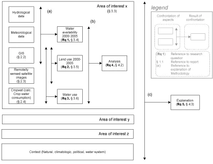
This section introduces the methods that were chosen to be applied for the research. These choices will be explained in this paragraph. This report is build up in the same way as the described methodology, so it forms also the guideline through this report.
figure 2.1: Methodology
In figure 2.1 the used methodology is shown. The way this methodology is built up will be explained now:
(a) These arrows show how the different ingredients of the research are linked to answer the research questions 1 to 3.
geographically determined aspects of this research area (water availability, water use, etc.) have to be combined to draw conclusions, the usage of a GIS is suitable for this research. The backgrounds of GIS’s are explained in paragraph 2.2.
The land use in the research area is determined by an analysis of remotely sensed satellite images. A land cover classification is carried out on these images to determine the areas of the different agricultural land uses. Land over classification is a suitable method to answer research question 2, because it is able ‘measure’ the land cover in a direct way on a large scale and to make a downscaling to focus areas which are relevant for this research. Besides this, land use data of local agricultural agencies are doubtful; political decision about growing a crop in a certain quantity and the real planted area of the concerning crop are not clear distinguishable. The results of the land cover classification and its theoretical backgrounds are respectively described in paragraph 3.5 and 2.3.
For calculating the irrigation water use (research question 3), the results of the land use analysis is combined with crop water requirements calculations. The used calculation software is Cropwat. The results of the irrigation water use calculations and information about Cropwat is given in the paragraphs 3.6 and 2.4.
The described efforts in step (a) will be carried out for different focus areas in the research area to satisfy the spatial aspect of the research. In paragraph 3.3 the borders of these areas, called ‘areas of interest’, are clarified.
(b) To answer research question 4 (“how are spatial explicit water availability, agricultural land use and irrigation water use related between 2000 and 2005 in different focus areas in the research area?”), the findings of research question 1 to 3 are analyzed per area of interest. This analysis will be carried out by a comparison of the inter-annual trends of water availability, agricultural land use and irrigation water use. This analysis is described in paragraph 4.2.
2.2
Geographical Information Systems (GIS)
This paragraph is derived from a course book aboutGIS (De By, 2004).
A geographical information system (GIS) can be defined as a computerized system that facilitates the phases of data entry, data analysis and data presentation especially in cases when we are dealing with georeferenced data. Data is georeferenced when coordinates from a geographic space have been associated with it. The georeferenced data tells us where the object represented by the data is (or was or will be). The main characteristics of a GIS software package are its analytical functions that provide means for deriving new geoinformation from existing spatial and ‘attribute data’ (see
glossary). In using GIS software we obtain some computer representations of the geographic phenomena which exist in the real world. Continuing with manipulating the data with techniques like ‘image classification’ (see paragraph 2.3) or overlaying to maps (layers) to retrieve a new map (see figure 2.2), results in additional computer representations. Since the spatial referencing is an important issue in GIS, a further explanation of topics which have to do with spatial referencing (georeferencing and resampling) is given in appendix 1.
These computer representations, existing of bits and bites, can be used for making visualizations, either on-screen, printed on paper, or otherwise. In this thesis the goal of making computer representations and visualizations of the real world, is to obtain additional data which are required for doing the analysis about the spatial relation between water availability and irrigation water use. The main technique used to obtain the research goal of this theses was ‘image classification’. To understand the principles of image classification, the reader of this master thesis has to know some basic concepts about ‘Remote sensing’. Backgrounds of remote sensing are explained in appendix 2 and ‘image classification’ will be explained in the following paragraph.
2.3
Image classification
2.3.1 Introduction
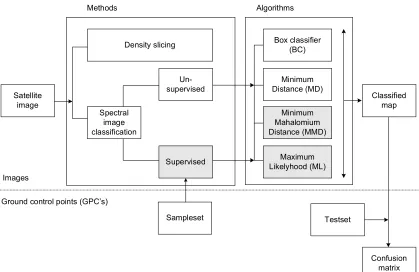
Sources for this paragraph are (Kerle et al., 2004), (Lillesand and Kiefer, 1994) and (ITC, 2001). Image classification is a sub area of Remote sensing. It is based on the different spectral characteristics of different materials on the earth’s surface and their reflection to a sensor. The overall objective of image classification procedures is to automatically categorize all pixels in an image into land cover classes or themes. Several image classification methods are available in literature. The most commonly used methods are: ‘density slicing’, ‘unsupervised spectral image classification’ and ‘supervised spectral image classification’. These methods will be discussed in the next sub-paragraphs. The scheme in figure 2.3 shows the main line of these sub-paragraphs. Sub-paragraph 2.3.6 will discuss some shortcomings of the selected method.
figure 2.2: Example of creating a new visualization. Two different layers can be
Density slicing
Spectral image classification
Un-supervised
Supervised Likelyhood (ML)Maximum Minimum Mahalomium Distance (MMD)
Minimum Distance (MD)
Box classifier (BC)
Classified map Satellite
image
Sampleset Testset
Confusion matrix Images
Ground control points (GPC’s)
Methods Algorithms
figure 2.3: Image classification methods and algorithms
2.3.2 Methods
Density slicing is a technique, whereby the Digital Numbers (DN-values, see appendix 2.7) distributed along the horizontal axis of an image histogram1, are divided into a series of user specified intervals or slices. Density slicing will only give reasonable results, if the DN-values of the cover classes are not overlapping each other.
In an unsupervised classification, clustering algorithms are used to partition the feature space2 into a number of clusters
In a supervised classification, the partitioning of the feature space is realized by an operator who defines the spectral characteristics of the classes by identifying sample areas (training areas). The operator needs to know where to find the classes of interest in the area covered by the image. This information can be derived from ‘general area knowledge’ or from dedicated field observations.
Important background information about classification methods is given in appendix 3.1.
Comparison of classification methods
Since the histograms of the individual bands and the histograms of the Normalized Defined Vegetation Indices do not show separate land cover classes, Density slicing is not an appropriate method to carry out an image classification (see appendix 3.1)
1 For definition, see Glossary
Since there was no land cover data of the area available the result of an unsupervised classification could not be validated. Therefore, this method was scientifically untenable. In combination with validation data the unsupervised classification could be useful. But when a field visit will be made and the expectance is that many sample data will be collected, it is more logical to choose for the supervised classification, since the basis of this method is the ‘real’ field data. Recapitulating: in the supervised approach we define useful information categories and then examine their spectral reparability; in the unsupervised approach we determine spectrally separable classes and then define their informational utility. Since many ‘useful information categories’ is collected during the field visit, the supervised classification was the most suitable classification method in this case.
2.3.3 Algorithms
After the training sample sets have been defined, classification of the image can be carried out by applying a classification algorithm. Several classification algorithms exist. The following algorithms will be explained, because they are well-known in literature and the used software package, ILWIS, allows only these methods to use for image classification: Box classifier (BC), Minimum Distance (MD), Minimum Mahalomium Distance (MMD), Maximum Likelihood (ML). See appendix 3, paragraph 3.2 for a detailed description of these algorithms.
To demonstrate and evaluate the results of these four methods, they are applied to the sample sets of the (2004_right). See table 2.1 for the accuracies of bananas, beans, paddy and water. How these accuracies are calculated will be explained later in sub-paragraph 2.3.4. In paragraph 3.5.2, ‘classification results’, the four methods will be applied to all sample sets and the final result of the land cover classification will be given then.
BC MD MMD ML
Banana (yellow) 0.38 0.44 0.84 0.81
Beans (brown) 0.40 0.74 0.74 0.75
Paddy (red and pink) 0.65 0.68 0.96 0.96
Water (blue) 0.91 1.00 1.00 1.00
Overall 0.86 0.95 0.99 0.99
table 2.1: Accuracies of algorithm methods for 2004_right
The accuracy of bananas is very low when BC and MD classifiers are used. The density and the distribution of the banana point-cloud is not taken into consideration in these methods. The un-dens cloud of beans (brown) and coco (light blue) are prevailing the banana (yellow), see figure 2.4. The low score of the accuracy of beans using the BC method can be explained by overleap of the beans by coco. In the BC and the MD method, paddy scores low. In figure 2.4 it can be seen that bare land (grey) is overleaping the point-cloud of paddy (red and pink). MMD and ML classifiers have better scores for paddy, because they are bringing the dens and concentrated character of the sample set of paddy into account.
Feature space of sample set Box classification Minimum distance classification
figure 2.4: Comparison classification algorithms for sample set of 2004_right
Threshold distance
Variation in threshold distance, explained in appendix 3, gave no improvement of the accuracy of the ML and MMD classifiers. ML classifications with a threshold distance of 100, 80, 60, 40, 20, 10 are carried out with the sample set of 2004_right and gave all an overall accuracy of 98.64%. This is the same as the overall accuracy in case no threshold distance is specified (see table 3.6) A threshold distance of 5 gave 98.63%, just 0.01% lower (!). Apparently, almost all feature vectors of the image do not fall far away from the mean values of the clusters. Therefore, the rest of the images are classified with a non-specified threshold distance.
2.3.4 Accuracy assessment of the classification result
“A classification is not complete until its accuracy is assessed” (Lillesand and Kiefer, 1994).
Banana Beans Coco Grass Paddy Water Unclass Accuracy
Banana 295 0 25 8 0 0 1 0.9
Beans 0 0 0 0 0 0 0 ?
Coco 0 0 0 0 0 0 0 ?
Grass 0 0 0 0 0 0 0 ?
Paddy 37 0 8 0 879 0 2 0.95
Water 0 0 0 0 0 3193 64 0.98
Reliability 0.89 ? 0 0 1 1
Average Accuracy 94.33
Average Reliability 96.33
Overall Accuracy 96.79
KHAT-value 92.76
table 2.2: Example of a confusion matrix (2003_right)
A confusion matrix gives a value for the accuracy and the reliability for each class. The accuracy is defined as: the fraction of correctly classified test set pixels of a certain ground truth class. For each class of test set pixels, the number of correctly classified pixels is divided by the total number of test pixels in that class. The reliability is defined as the fraction of correctly classified test set pixels of a certain class in the classified image. For each class in the classified image (column), the number of correctly classified pixels is divided by the total number of pixels which were classified as this class. Also statistics to assess the accuracy and reliability of the whole classification are available: the average accuracy, the average reliability, the overall reliability and the KHAT-value. In appendix 3, paragraph 3.3 a more detailed explanation is given about the main concepts of a confusion matrix.
2.3.5 Sample set and test set
A part of the total retrieved ground truth data about land covers, in the case of this thesis agricultural field with a certain crop, has to form the test set. The other part will be the sample set. The first consideration is: “when can an agricultural field be part of the ground truth data?” The second question is: “how many sample areas are required?” The last point to discuss in this context is: “which part of the total amount of test areas should form the test set?
Ground truth data
Amount of sample areas
Different guidelines for the size of a sample set are given in literature.
• A minimum of 50 sample areas per class in the case of a few different classes and 75 to
100 per class in the case of 12 classes or more (Lillesand and Kiefer, 1994).
• A minimum of 30 sample areas per class (Kerle et al., 2004).
The conditions in each research area are different, so these quantities are just guidelines. Besides this, not any class has the same variability. ‘Water’ for example, requires less sample areas than banana, which can vary in grow stage.
Division sample set – test set
The ground truth data set has to be separated in a sample set and a test set. Which fields should be part of the test set and how many? Systematically sampling or random sampling are the two main options. In systematically sampling, only the field with a high level of certainty are selected for the test set. Random sampling selects random field for the test set. Because the amount of the ground truth data in this thesis is limited, the systematically way of sampling is applied. The relation sample set : test set in these thesis is 1:4. This division key is commonly used.
2.3.6 Shortcoming of image classification
Processing of the training set results in spectral classes. Sometimes these spectral classes are not equal to the real classes in consideration. For example: banana fields do not give the same spectral reflectance, due to differences in grow stage, banana type and ground type.
Another main problem is the existence of ‘mixels’. Each pixel in a classified image can only represent one land cover class. In reality, more than one land cover can occur within one pixel. The reflectances of these different cover classes are mixed to one DN-value per band. The result of this phenomena is called a mixel. For example: when the pixel covers the border of an agricultural field and the road besides. In the case of this thesis, this is an important point of consideration, because the pixel sizes of the used images are 20 m and 30 m.
2.4
Irrigation water use
2.4.1 Introduction
Since no data are available about quantities of irrigation water used for growing crops in the research period, the irrigation water use has to be derived from other parameters. This paragraph will explain the used calculation methods to calculate the irrigation water use of crops. Firstly the physical phenomenon of transpiration and soil moisture will be explained. Thereafter the chosen method for calculating the irrigation water use of a crop will be clarified.
2.4.2 Soil-plant-water relationships
This sub-paragraph is derived from Bailey (1990).
as the ‘actual transpiration rate’. The driving force which determines this is the weather, but it is also regulated by the type of crop and the availability of moisture in the soil. It is increased by bright sunshine, high temperatures or strong winds.
The basic model, used in irrigation, is that the soil under constant conditions contains a constant amount of water; called the ‘field capacity’. The force holding the water is called ‘surface tension’. As a crop removes water from the soil, the soil is described as having a certain soil moisture deficit (SMD). The SMD at field capacity is zero. If a crop extracts 50 mm of water from a soil, and there has been no rainfall or irrigation to replenish it, the soil is said to have an SMD of 50 mm. When there is no restriction on soil moisture, and the rate for a given crop is determined solely by the weather, it is said to be proceeding at its full potential which is referred to as the potential transpiration rate. When the SMD increases, the actual transpiration of a crop may fall below the potential transpiration because the crop reacts on the lack of soil moisture by closing its tiny transpiration holes. The SMD at which this occurs is called the ‘critical SMD’. In most situations the objective of irrigation is to keep the SMD below the critical level.
2.4.3 Calculating the irrigation water use by using Cropwat
Cropwat (FAO, 1992) is a computer program for irrigation planning and management. It is a commonly used method to give estimations about crop water requirement without requiring many measurements (many standard values of, for example, climate conditions are available as input for Cropwat). Since there is a little knowledge about each particular agricultural field in the research area, Cropwat is a suitable method for calculating the crop water requirements in the research area. It is not the aim of this study to evaluate the working of Cropwat. Therefore, the calculations methods of Cropwat will be briefly discussed. This brief description is mainly taken from the ‘water report nr 22’ of FAO (FAO, 2000)
Cropwat calculates the transpiration (T) of a crop and the evaporation (E) of the soil of an agricultural field, together called the evapotranspiration (ET). The calculation of a reference evapotranspiration (ETo) is based on the FAO Penman-Monteith method (FAO, 1998). Input data include monthly and ten-daily for temperature (maximum and minimum), humidity, sunshine, and wind-speed. Crop water requirements (ETcrop) over the growing season are determined from ETo and estimates of crop evaporation rates, expressed as crop coefficients (Kc), based on well-established procedures (FAO, 1977), according to the following equation:
0
ET
K
ET
crop=
c×
Through estimates of effective rainfall (taking into account that a part of the rain runs off), crop irrigation requirements are calculated assuming optimal water supply. Inputs on the cropping pattern will allow estimates of scheme irrigation requirements. With inputs on soil water retention and infiltration characteristics and estimates of rooting depth, a daily soil water balance is calculated, predicting water content in the rooted soil by means of a water conservation equation, which takes into account the incoming and outgoing flow of water.
It is assumed that the crops in the research area are irrigated in an efficient way, that is: refilling the soil water content to field capacity when the critical SMD is reached. By doing this assumption, Cropwat can be used to calculate the irrigation water use of the crops in the research area.
3
Data processing
3.1
Introduction
This chapter deals with the processing of rough data to a format which is suitable for answering the research questions 1 to 3 about the evolving of water availability, agricultural land use and irrigation water use. Firstly the period of interest and the area of interest will be further specified to focus the efforts of translating the available data to the goal of study. Thereafter, the way the water availability, the land use and the irrigation water use is quantified will be explained in respectively paragraph 3.3, 3.4 and 3.5. These paragraphs will be the ingredients for the next chapter: Results.
3.2
Period of interest
Three factors are important to consider to make a choice for a suitable period of interest.
Firstly, it has to be a clear-cut period in which the phenomena of the problem this thesis is dealing with -explaining the inter-annual dynamics of irrigation water use and land use under different water availabilities- are clearly come up. From the field work it is known that the research area knows two of these clear-cut periods: the dry season and the wet season. In the dry season, the scarcity of water is larger than in the wet season. It is expected that in this period the expected relations between the behavior of land use, irrigation water use and water availability become more clear distinguishable than in the wet season.
Secondly the grow season is important, since the crops are the actual irrigation water users. The period of interest should start when the earliest crop in the dry season is planted and it should stop when the last crop in the dry season is harvested.
Finally, the availability of data is an important point of concern. Since this research uses a land cover classification, cloudless satellite images are required. Only in the dry season cloudless images were available.
Resuming the issues pointed above, the period of interest starts when the first crop in the dry season is planted and ends when the last crop is harvested. This is approximately from June up to December.
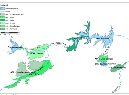
3.3
Areas of interest
AOI 4: Trussu
AOI 2: River
AOI 3: Orós
AOI 1: Locally stored runoff
AOI 6: Perímetro AOI 5: Lima Campos
Jaguar
ibe
Salg a do
Trus s u river
Jag/Trussu river
Tunn el
Orós reservoir
Trussu reservoir
Lima Campos reservoir
Legend
Reservoirs (2000) Rivers
AOI 1: Locally stored runoff AOI 2: River AOI 3: Orós AOI 4: Trussu AOI 5: Lima Campos AOI 6: Perímetro
0 2.5 5 10
Km
figure 3.1: AOI’s
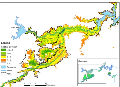
3.3.1 AOI 1: Locally stored runoff
It is mentioned in sub-paragraph 1.2.3 that studies about runoff reached the conclusion that, in the crystalline areas of the Semi-Arid zone of Brazil, an average of only 6 to 8% of the rainfall actually flows superficially or feeds aquifers by percolation. During the field visit, several plots irrigated by this kind of stored runoff have been visited (see figure 3.2).
These plots were concentrated in the area between the Trussu reservoir and the Jaguaribe river. A ‘relative elevation’-map, as drawin in figure 3.3, gives more insight in the question why these area uses locally stored runoff. ‘Relative elevation’ is defined as the elevation of a location minus the elevation of nearest point of the river. How the relative elevation is determined is
AOI 2: River
AOI 3: Orós
AOI 4: Trussu
AOI 1: Locally stored runoff
Trussu reservoir
Text
Overview Legend
Relative elevation
-10 - -3 -3 - 0 0 - 3 3 - 6 > 6 Reservoirs Rivers AOI's
0 2.5 5 10
Kilometers
figure 3.3: Relative elevation perpendicular to river
It can be read in figure 3.3 that the relative elevation in the northern cross-direction of the Jaguaribe river first increases and subsequently decreases in the form of two ‘bowls’. So two local depressions can be seen in which the relative elevation to the river decreases to -6 m.
Another property of this area is that the upper part of the soil has mainly an alluvial soil or a vertisoil (see the graph of AOI 1 figure 3.4 ‘soil types per AOI’). These soil types are called ‘heavy’, which means that it contains fine particles like clay and has a good water holding capacity.
The third point of attention is that water wells and natural lakes were observed in this area. The lakes originate in the center of these local depressions. Two reasons can be given for this phenomenon: either the surface intersects the groundwater table or the rainwater of the wet season is retained by the soil. Since lack of data about groundwater tables and the existence of aquifers, this will not be investigated further. Together with the knowledge that the distance to the Trussu river and the Jaguraribe river is to large to get water from there, it is assumed that this area gets water from locally stored runoff.
figure 3.4: Soil types per AOI A O I 4: T ru s s u A O I 2: R iv e r A O I 3 : O ró s A O I 1: L o ca lly s to re d r u n o ff A O I 6: P e rí m e tr o A O I 5: L im a C a m p o s L e ge nd R es er vo ir L im a C am p os R es er vo ir O ró s B ro w n w ith ou t c a lc iu m La ke d o B a ú La to so il R ed D is tr of ic 7 P la no so il S o ló d ic o T a2 P o ds oi l R ed Y e llo w S o il lit o lic E ut ro fic a nd D is tr o fic 1 1 S o il lit o lic E ut of ic a nd D is tr o fic 1 4 S o lo n et z S o lo d iz a do 6 S o il A llu vi a l E u tr of ic V er tis o il S oi ls A O I 5 0 20 0 40 0 60 0 80 0 10 00 12 00 Re se rvo ir Lim a Ca m po
s il LSo
ito lic E utr ofi c 1 So il A llu via l E utr of ic 16 Ve rti so il 1 1 Ve rti so il 1 6 S o ils Are a ( ha ) S o ils A O I 3 0 10 00 20 00 30 00 40 00 50 00 60 00 70 00 80 00 Re se rv oir O ró s Po ds oi l R ed -Y el lo s Eu tro fic 5 5 So il Li to lic E ut ro fic 3
8 rtiVe
ss ol o1 3 Ve rti so il 7 S o ils Are a ( ha) S o ils A O I 6 0 20 0 40 0 60 0 80 0 10 0 0 12 0 0 14 0 0 16 0 0 18 0 0 So il Li to lic E ut ro fic 4 2 So il Al lu via l E ut ro fic 1 8 Ve rti so il 7 S o ils Are a ( ha)
S
o
il
ty
p
es
p
e
r
A
O
I
S oi ls A O I 1 0 50 0 10 00 15 00 20 00 25 00 30 00 35 00 4000 keLa
d o Ba ú Pl an os so lo S ol ód ic o Ta 2 Po ds oi l R ed -Y el los E ut ro fic 2
3 il LSo
ito lic E ut ro fic
14 il So
Al lu vi al Eu tro fic
4 il ASo
3.3.2 AOI 2: Water from river (Jaguaribe)
The map in figure 3.3 can also be used to determine the areas that have access to water from the river. During the field visit it became clear that the water from the river is pumped to the areas around the river. From information retrieved from local farmers the pumps used can pump the water up to around 6 meters, the area of AOI 2 is determined by this rule: relative elevation to the river = 6 m.
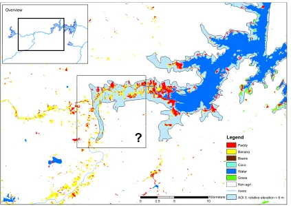
3.3.3 AOI 3: Edge Orós reservoir
Similar to AOI 2, farmers at the edge of the Orós reservoir also pump up the water to their agricultural fields. To obtain a suitable area in which the agricultural fields are supplied by only reservoir water, a same kind of decision rule to determine the border as in AOI 2 can be used. A problem comes up when a fixed relative elevation rule is applied: at the location where the Jaguaribe/Trussu river enters the Orós reservoir, the borders drawn by the fixed relative elevation rule are too far away from the reservoir to make it reasonably possible to pump the water from the Orós reservoir to these areas (see the box marked with a question mark in figure 3.5. How this land use map is made will be explained in 3.5).
This figure shows also that in other areas on the reservoir edge, the rule ‘relative elevation = 6 m covers the suspected areas supplied by reservoir water.
Overview
Legend
Paddy Banana Beans Coco Water Grass Non-agri rivers
AOI 3: relative elevation = 6 m
0 2.5 5 10
Kilometers
?
figure 3.5: Border AOI 3 in 2005 due to relative elevation from the reservoir level of 6 m
With the available information (land use data, DEM, discharge data, reservoir data) it is hard to determine where the exact border between fields that are supplied by water from the river and water from the Orós reservoir has to be drawn. So an estimation has to be made. The following points are considered in this estimation:
1. The satellite images show agricultural activity in the surrounding of the river. Other
types of water availability, besides the reservoir water, can therefore not be neglected in the dry season.
2. In a land use classification map as shown in figure 3.6 , it can be seen that water in the
Jaguaribe/Trussu river during the dry season is dammed by little dams in the river bed. Upstream from these little dams, small reservoirs in the river bed emerge. It is assumed that agricultural fields around such small reservoirs are supplied by water from these small reservoirs and not by water form the Orós reservoir.
3. When the small reservoirs are close to the Orós reservoir and close to each other it is
assumed that the water from the Orós reservoir is pumped up from reservoir to reservoir. This is a hypothesis, not an observation from the field visit.
4. When the shape of the fields are clearly rectangular and perpendicular to the river, it is
assumed that they are supplied by water stored in the river bed.
Overview Legend
Paddy Banana Water Non vegetation aoi_oros_2005
0 0.5 1 2
Kilometers
figure 3.6: Boundary of AOI 3 in 2005 at inlet point
figure 3.7: AOI 3 in each year
2
00
0
20
05
2
00
4
20
0
3
2
00
1
2
00
2
0 10 20 5 K ilo m et e rsA
O
I 3
: R
e
se
rv
oi
r
e
d
ge
O
ró
s
2
00
0-2
00
5
L eg end Paddy Banan
Points of discussion:
• It is questionable how far the pumps can transport the water in horizontal way. In the
drawn borders, this distance is around 2,5 km. Extra information about this distance should make it possible to draw a more certain border.
Since the water level of the reservoir is changing during the dry season (it is decreasing, see figure 3.11), also the area of interest is changing during the dry season according to the fixed elevation difference determined by the pumps. Since the goal is to determine a fixed AOI per dry season, a reference water level had to be chosen. The acquisition date of the satellite images is chosen as date for the reference water level, since the land use maps, which are derived from these satellite images with a certain acquisition date, are also used to determine the borders (as described above). A fixed elevation difference form the water level (which is decreasing in the dry season) makes the water level at the end of the dry season determinative for the areas than can be supplied by water during the whole season. Since the acquisition dates of the satellite images are at the end of the dry season (21 October – 13 November) they are useful for this goal. In figure 3.7 it becomes clear that the fields around the reservoir edge are included in AOI 3 by using these reference dates, which makes these dates suitable for determining the borders of AOI 3.
• The water level at the acquisition dates could be determined in two ways: crossing the
DEM with the satellite image and reading the elevation of the pixels at the water edge or converting the available daily volume data (COGERH, 2005) with a given ‘volume-water level’-relationship. In each year the difference between both methods was around 6 m (see table 3.2). Probably the reference of one of both data sources is not correct.
• The difficulty to determine the border at the inlet of the Orós reservoir (area with
question marked in
• figure 3.5) gives this area of interest the most uncertainty. In chapter 5, Discussion, this
border will be varied to see the impact of this uncertainty on the conclusions of this research.
Year Water level in DEM (m) Water level in COGERH data (m) Difference DEM – COGERH (m)
2000 196 191 5
2001 192 185 7
2002 192 185 7
2003 195 188 7
2004 204 198 6
2005 203 197 6
Mean ≈6
table 3.1: Water level data of DEM and COGERH (2006)
3.3.4 AOI 4: Downstream of Trussu reservoir
The area from the joining point of the Jaguaribe river and the Trussu river to AOI 3 can be supplied by three sources: discharges from the Jaguaribe, releases from the Trussu river and water from the Orós reservoir (due to the uncertain border of AOI 3). Therefore, this area was not suitable for joining AOI 4 or to form an extra AOI (see also 3.3.7).
3.3.5 AOI 5: Edge Lima Campos reservoir
The Lima Campos reservoir is supplied by a tunnel/canal from the Orós reservoir. From the outlet of the tunnel, two main canals are lead to the Lima Campos reservoir. The agricultural fields north of the Lima Campos reservoir are supplied by water from these canals. The agricultural field west of the Lima Campos reservoir are not supplied by these canals. Since the AOI’s are assumed to be areas with one main water source, the areas which are supplied by the canals are selected. The boundaries of AOI 5 are determined by the location of the outlet of the tunnel (recorded by GPS) in combination with the elevation map and observations during the field visit (see figure 5.2 in Appendix 5).
3.3.6 AOI 6: Downstream Lima Campos reservoir, irrigation scheme
The boundaries of AOI 6 are determined by the irrigation scheme which contains fixed locations of fields. The fixed network of cannels gets its water from the release from the Lima Campos reservoir by operations of the dam.
3.3.7 Remaining points of consideration
3.4
Water and land availability data
3.4.1 PrecipitationSource of data
The rainfall data is obtained from FUNCEME (FUNCEME, 2006). A selection had to be made since some rain stations gave empty-values for certain periods. Per year is examined which rain stations were operative; the operative rain stations were used. In figure 3.8 the operative rainfall stations of 2000 are shown.
Conversion to mean monthly data per AOI
The daily rainfall data is converted to monthly rainfall
data, since this scale fits better to the scale of the research and Cropwat, the software that is used for determining the irrigation water use, is using the same scale for the input of rainfall data. The monthly point data is interpolated to give each pixel in the research area a rainfall value. Several interpolations methods were available in the used software (Budde et al., 2005):
- Thiessen (each pixels is attributed the value of the closest rainfall stations)
- Moving average (each pixel-value is determined by the weighted average of the surrounding rainfall stations)
- Surface (One polynomial surface is calculated by a least squares fit through the values of all rainfalls stations. A value, related to this surface, is assigned to each pixel in the map) - Kriging (similar to moving average but the weight factor is not determined by the
distance to a rainfall stations, but by a user-specified semi-variogram)
Since the interpolation had to be done 72 times, a simple method was preferable. The Thiessen method and the Moving average method can be marked as simple method, since a few input variables are required. To decide which of both method to choose, the rainfall stations of a representative month are divided in a sample set and a test set. Both methods are carried out on the sample set and the results are compared with the test set. The representative month was December 2001. The year 2001 had the most operative rainfall stations (19) in the period 2000-2005, so a division in a test set and a sample set left enough points for the sample set to carry out the interpolations. Since the test set counts only 4 rainfall stations, the ratio of error can be remarkably vary by different test sets. Therefore, this calculations is carried out in 3 with different test sets. The results are shown in table 3.2. Since the Moving Average method scores better over these three test sets, this method is used for all interpolations.
The ‘ratio of error’ is calculated by:
85 65
88 46
66
81
65
52.8
86.8
Legend
Rivers reservoirs (2000) rainfall stations
02.5 5 10
Kilometers
4
%
100
4
1
∑
=
×
−
=
n nn n
T
T
S
ratio
With:
n = rainfall stations of test set
Sn = Result of interpolation of sample set at location n
Tn = Measured rainfall at location n
Test set Ratio of error Nearest Point (%) ratio of error Moving Average (%)
1 24 18
2 35 36
3 30 11
table 3.2: results of error of interpolation methods rainfall
Figure 6.1 in appendix 6 shows, as example, the result of the interpolation of the monthly rainfall data of December 2000 using the Moving Average method, figure 6.2 of appendix 6 illustrates the mean rainfall per AOI. The graph of figure 3.9 shows the monthly rainfall per AOI. The results show in some years a high variation between different AOI’s: the wet seasons of 2003 and 2004 show in some months a variability around 150 mm. This result confirms the temporal and spatial variation in the area, that as concluded in sub-paragraph 1.2.1.
Monthly Rainfall per AOI
0 100 200 300 400 500 600
Tim e (months)
M
o
n
th
ly
R
a
in
fa
ll
(
m
m
)
AOI 1 Groundwat er AOI 2 River AOI 3 Orós AOI 4 T russu AOI 5 Lima Campos AOI 6 Perímet ro
figure 3.9: Monthly rainfall per AOI
Reliability of rainfall data
3.4.2 River discharge Icó Orós Trussu Iguatú LimaCampos Outlet tunnel Orós
Legend
Dischargepoints Reservoirs (2000) Rivers
AOI's
AOI 1: Locally stored runoff AOI 2: River AOI 3: Orós AOI 4: Trussu AOI 5: Lima Campos AOI 6: Perímetro
0 5 10 20
Km
Discharges at Icó and Iguatú
0 50 100 150 200 250 300 350 Ja n-00 Ju n-00 De c-00 Ju n-01 De c-01 Ju n-02 De c-02 Ju n-03 De c-03 Ju n-04 Date D is ch ar g e (m 3/ s) Ico Iguatu
Discharges at Trussu, Orós and Lima Campos
0 2 4 6 8 10 12 14 Ja n-00 Ju n-00 De c-00 Ju n-01 De c-01 Ju n-02 De c-02 Ju n-03 De c-03 Ju n-04 De c-04 Ju n-05 No v-05 Date D is ch ar g e (m 3/
s) TrussuLimacampos
Oros Tunnel
figure 3.10: Discharges
Source of data
Discharge data at the dams of Orós, Lima Campos and Trussu and discharge data of the tunnel between the Orós reservoir and the Lima Campos reservoir were recorded by COGERH (COGERH, 2006), the organization responsible for the management of the water recourses in the area. Discharge data at Iguatú, along the Jaguaribe river, and Icó, along the Salgado river, were available by CPRM, (CPRM, 2006), which is the geographical service in Brazil. The data of these 6 measurement stations were recorded with a temporal resolution of 1 month. In 2004, daily data was available at the dams.
Discharge data in the Jaguaribe and Salgado rivers of 2005 was not available at the moment of writing this thesis.
Reliability of river discharge data
The river discharge data at Icó and Iguatú are the result of a measurement with a stage-discharge relationship; the stage is constantly measured and the discharge is calculated using the stage-discharge relationship. This relationship is among other things dependent of the geometry in the cross-direction of the river. Since the riverbed of river is constantly changing, especially in a river that has a high variability in discharge like the Jaguaribe, this relationship has to be constantly updated (Shaw, 1994). The stage-discharge relationships at Icó and Iguatú are expected to be regularly updated. The frequency and the method of updating the stage-discharge relationship are unknown. Since this is the only discharge data