DOOMRED: A New Optimization Technique for Boosted Cascade Detectors on Enforced Training Set

(1)

Volume 2008, Article ID 183804,11pages doi:10.1155/2008/183804

Research Article

DOOMRED: A New Optimization Technique for Boosted

Cascade Detectors on Enforced Training Set

Dong Woo Park1_{and Kyoung Mu Lee}2

1_Information_&_{Technology Laboratory, LG Electronics Institute of Technology, 16 Woomyeon-dong, Seocho-gu, Seoul 137-724, Korea}

2_{Department of Electrical Engineering, ASRI, Seoul National University, 599 Gwanangno, Gwanak-gu, Seoul 151-742, Korea}

Correspondence should be addressed to Kyoung Mu Lee,[email protected]

Received 31 August 2007; Revised 27 December 2007; Accepted 19 February 2008

Recommended by Olivier Lezoray

We propose a new method to optimize the completely-trained boosted cascade detector on an enforced training set. Recently, due to the accuracy and real-time characteristics of boosted cascade detectors like the Adaboost, a lot of variant algorithms have been proposed to enhance the performance given a fixed number of training data. And, most of algorithms assume that a given training set well exhibits the real world distributions of the target and non-target instances. However, this is seldom true in real situations, and thus often causes higher false-classification ratio. In this paper, to solve the optimization problem of completely trained boosted cascade detector on false-classified instances, we propose a new base hypothesis weight optimization algorithm called DOOMRED (Direct Optimization Of Margin for Rare Event Detection) using a mathematically derived error upper bound of boosting algorithms. We apply the proposed algorithm to a cascade structured frontal face detector trained by AdaBoost algorithm. Experimental results demonstrate that the proposed algorithm has competitive ability to maintain accuracy and real-time characteristic of the boosted cascade detector compared to those of other heuristic approaches while requiring reasonably small amount of optimization time.

Copyright © 2008 D. W. Park and K. M. Lee. This is an open access article distributed under the Creative Commons Attribution License, which permits unrestricted use, distribution, and reproduction in any medium, provided the original work is properly cited.

1. INTRODUCTION

Recently, the boosted cascade detector [1] became the most popular method for an object detection in computer vision. Due to its accuracy and real-time characteristic, many works have been proposed to enhance the original one [2–4]. However, most researches on the boosted cascade detector have concentrated on the learning problem for a fixed number of initial training data. The basic assumption made in the researches is that the distributions of the target and nontarget objects obtained from the given fixed number of initial training data are good enough to reflect the real distributions, which is seldom true in practice. This is because it is almost impossible to know the exact distribution of the target as well as nontarget instances in real situations. As a result, the detector trained with the fixed number of initial training data cannot work properly in the real applications.

The problem we would like to address in this paper is “what should be done to a completely trained object

(2)

resulting overall great amount of computational burden in real applications.

To overcome these diﬃculties, the optimization algo-rithm for a boosted cascade detector on an enforced training set needs the following three conditions:

(1) an explicit optimization rule guaranteed by the math-ematical background,

(2) less optimization time than the time for the retraining, (3) low false positive rate while maintaining the expected

detection rate for a given target training set.

In this paper, we propose a fast algorithm called DOOM-RED (direct optimization of margin for rare event detection) that optimizes the base hypothesis weight set of each single layer detector in a boosted cascade detector, especially when the false-rejected target instances are enforced. Note that, in a boosting algorithm, the base hypothesis selection procedure from the large candidate base hypothesis set usually demands high-computational cost. This is the reason why we focus on the optimization of the base hypothesis weight set for the performance enhancement of a boosted cascade detector. In this respect, DOOMRED may be categorized as a kind of back-fitting which is a well-known optimization algorithm in the machine learning field [5].

2. BOOSTING ALGORITHM

Boosting is a well-known machine learning method that constructs a binary classification rule from certain training data set. The basic idea of a boosting algorithm is somewhat simple though clear such that an ensemble combination of multiple base hypotheses makes one strong hypothesis. The base hypothesis means a classification rule which has slightly better accuracy than random choice on a given training data set, which has error slightly less than 0.5. Meanwhile, the strong hypothesis indicates a classification rule that has high accuracy on the given training data set. Because constructing a highly accurate classification rule at one try is hard, a boosting algorithm constructs one accurate classification rule by combining multiple classification results from several base hypotheses. At this point, two important issues will be what base hypotheses to select from abundant candidate base hypothesis set, and how to combine them to make one accurate classification rule. In a learning procedure, both the training data setSand the candidate base hypothesis setH

should be predefined. Then, forTiterations, corresponding base hypotheses h ∈ H are selected sequentially from the candidate base hypothesis set H by updating the weight distribution of the training instances contained inSusing an implicit cost function. The merit of the boosting algorithm is that the selection procedure of the base hypothesis can compensate the performance of the previously selected base hypotheses. If an instance is classified correctly by the base hypothesis selected in previous iteration, its weight decreases and vice versa. By updating the importance of each instance for every iteration, a base hypothesis that has good accuracy on instances not correctly classified by previously selected base hypothesis is selected. AfterTiterations,Tbase hypotheses are selected and the final classification rule is

obtained by a linear combination (or ensemble combination) of T base hypotheses. The final outcome of the boosting algorithm is a binary classification rule f(x) on the test instancex, which is labeled byy∈ {−1, 1}as shown in (1) where T_i=₁wi = 1,wi > 0,hi(x) ∈ {−1, 1}. We limit our work in the range of boosting algorithms which deal with hypotheseshhaving only binary outputs−1 and 1:

f(x)=

T

i=1

wihi(x)=

≥θT, x∈class 1 (target),

< θT, x∈class 2 (non-target). (1)

Note that each of the finally selected base hypothesishi corresponds to a basis of the feature space where instances are distributed, and the set of T base hypotheses’ weight set is a gradient of a linear decision boundary. For this reason, the training procedure of a boosting algorithm can be interpreted as “data dimension reduction,” that is selecting base hypotheses which makes the distribution of class 1 (y= −1) and class 2 (y =1) instances in feature space separable with a linear decision boundary.

When f(x) is used as a general binary classifier, the thresholdθT =0. However, when f(x) is used as a rare-event detector such as a frontal face detector,θTis usually set in the range−1< θT ≤0. This is to guarantee the detection rate of

f(x) to be a specific goal value.

3. SINGLE LAYER DETECTOR OPTIMIZATION

3.1. Problem statement

(3)

0 0.2 0.4 0.6 0.8 1

Cθ

(

m

)

−1 −0.5 0 0.5 1

m(margin) (a)

0 0.2 0.4 0.6 0.8 1

Cθ

(

m

)

−1 −0.5 0 0.5 1

m(margin) (b)

Figure1: (a) Mean-shifted sigmoid function in (13) whenθ=0.5. (b) Digitized version of (a) when the margin is segmented in the size 0.25.

a boosting algorithm when large training set is given requires substantially long training time. To train a boosted frontal face cascade detector, the size of training data set should be about several ten thousands because training set should include all instances that represents the face’s large variance in appearance. For the frontal face detection problem, the training time for a cascade detector is minimally about several days using the fastest source codes such as OpenCV and maximally several weeks [1]. So, retraining cascade detector for every time when some instances are enforced is impractical. Second heuristic solution is to adjust the thresholdθT of each subdetector to make each one satisfies the specific goal detection rate as in (1). One obvious drawback of this approach is that the solution also increases the false positive rate exponentially. This will result in decreasing the detection speed of the whole cascade detector in real applications.

To overcome the shortcomings of the two heuristic solutions, in this work, we proposed a new optimization method for subdetectors in a boosted cascade detector that can minimize the false positive rate while maintaining the goal detection rate in reasonably small amount of

0.5 0.6 0.7 0.8 0.9 1

0 1 2 3 4 5 6 7 8

×10−3

Test false positive rate

Te

st

d

et

ec

ti

o

n

ra

te

1000 original target instances, 200 base hypotheses

DOOMRED Re-trained

Threshold adjusted Original detector (a)

0.5 0.6 0.7 0.8 0.9 1

0 1 2 3 4 5 6 7 8

×10−3

Te

st

d

et

ec

ti

o

n

ra

te

DOOMRED Re-trained

Threshold adjusted Original detector (b)

0.5 0.6 0.7 0.8 0.9 1

0 1 2 3 4 5 6 7 8

×10−3

Te

st

d

et

ec

ti

o

n

ra

te

DOOMRED Re-trained

Threshold adjusted Original detector (c)

(4)

0 0.1 0.2 0.3 0.4 0.5 0.6 0.7 0.8 0.9 1

0 0.2 0.4 0.6 0.8 1 Test false positive rate

Te

st

d

et

ec

ti

o

n

ra

te

3 base hypotheses, 2000 original target instances

DOOMRED Re-trained

Threshold adjusted Original detector (a)

0.5 0.6 0.7 0.8 0.9 1

0 1 2 3 4 5 6 7 8

×10−3

Te

st

d

et

ec

ti

o

n

ra

te

100 base hypotheses, 2000 original target instances

DOOMRED Re-trained

Threshold adjusted Original detector (b)

Figure3: The ROC curves of the single layer detectors when the detector contains (a) 3 (b) 100 (c) 200 base hypotheses.

optimization time. Our basic idea is to optimize the decision boundary of each subdetector only. The reason is that the most portion of training time of the boosting algorithm comes from base hypothesis selection procedure. Sections3.2

and3.3describe a mathematically derived optimization rule and an optimization algorithm that we propose.

3.2. Optimization rule

In this section, an upper bound on test error of the classification rule f(x) in (1) is derived in a more generalized form than the work in [6]. Based on the derived equation, the factors that aﬀect the accuracy of the boosted detector may be extracted. Then, by adjusting the controllable factors, the boosted detector can be optimized on the enforced training set.

Since the AdaBoost algorithm was proposed [7], it has been shown from the subsequent experiments that the

0.5 0.6 0.7 0.8 0.9 1

0 1 2 3 4 5 6 7 8

×10−3

Te

st

d

et

ec

ti

o

n

ra

te

DOOMRED Re-trained

Threshold adjusted Original detector 10 enforced target instances,

(a)

0.5 0.6 0.7 0.8 0.9 1

0 1 2 3 4 5 6 7 8

×10−3

Te

st

d

et

ec

ti

o

n

ra

te

DOOMRED Re-trained

(b)

0.5 0.6 0.7 0.8 0.9 1

0 1 2 3 4 5 6 7 8

×10−3

Te

st

d

et

ec

ti

o

n

ra

te

DOOMRED Re-trained

(c)

(5)

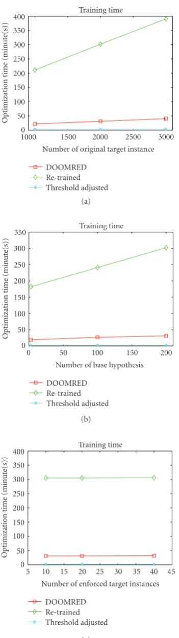
0 50 100 150 200 250 300 350 400

Optimizatio

n

time

(min

u

te(s))

1000 1500 2000 2500 3000 Number of original target instance

DOOMRED Re-trained Threshold adjusted

Training time

(a)

0 50 100 150 200 250 300 350

Optimizatio

n

time

(min

u

te(s))

0 50 100 150 200

Number of base hypothesis DOOMRED

Re-trained Threshold adjusted

Training time

(b)

0 50 100 150 200 250 300 350 400

Optimizatio

n

time

(min

u

te(s))

5 10 15 20 25 30 35 40 45 Number of enforced target instances

DOOMRED Re-trained Threshold adjusted

Training time

(c)

Figure5: The optimization time for the case in (a)Figure 2, (b) Figure 3, (c)Figure 4.

gap between the training error and test error decreases as the number of selected base hypotheses increases even after the training error reached to zero. These results show that the AdaBoost algorithm does not fit to the basic machine learning theory, Occam’s razor, saying that the classification rule should be as simple as possible to minimize the gap between the training error and test error. To explain this phenomenon, the upper bound on error of voting methods such as the AdaBoost algorithm has been derived mathematically in [6].

However, the upper bound derived in [6] works only for the general binary classification problem, whenθT=0 in (1). To make the upper bound on error of the boosting algorithm applicable even for the rare-event detection problem (when

−1 < θT ≤ 0), we derive a more generalized error upper bound inTheorem 1. So, (2) can be used as an upper bound of the false positive rate in real applications whenθTis tuned in the range−1 < θT ≤ 0 to get a specific goal detection rate. The proof is given afterTheorem 1following the similar procedure in [6].

Theorem 1. LetPbe a distribution over(x,y),y∈ {−1, 1}, and letSbe a set ofkexamples chosen independently at random according to P. Assume that the base hypothesis space H is finite, and let δ > 0. Then with the probability of at least

1 −δ over the random choice of the training set S, every function f made as a combination of h ∈ H satisfies the following bound for all −1 < θT ≤ 0, 0 < θ < 1, and 0<−θT+θ <1:

PrP

y f(x)≤ −θT

≤PrS

y f(x)≤ −θT+θ

+O

1

√

k

logklog|H|

θ2 + log

1

δ

1/2

.

(2)

Proof. For the sake of the proof, we defineCN to be the set of unweighted average overNelements fromH:

CN = f :x→ 1

N

i=1

hi(x)|hi∈H

. (3)

We allow the sameh ∈ H to appear multiple times in the sum. This set will play the role of the approximating set in the proof.

Any majority vote classifier f ∈ C can be associ-ated with a distribution over H as defined by the coef-ficients wi. By choosing N elements of H independently at random according to this distribution, we can gen-erate an element of CN. Using such a construction, we map each f ∈ C to a distribution Q over CN. That is, a function g ∈ CN distributed according to Q is selected by choosing h1,. . .,hN independently at random according to the coeﬃcients wi and defining g(x) = (1/N)N_i=₁hi(x).

Our goal is to upper bound the generalization error of

(6)

PrP

y f(x)≤ −θT

≤PrP

yg(x)≤θ

2

+ PrP

yg(x)>θ

2,y f(x)≤ −θT

.

(4)

This holds because, in general, for two eventsAandB,

Pr[A]=Pr[B∩A] + Pr[B∩A]≤Pr[B] + Pr[B∩A].

(5)

As (4) holds for anyg∈CN, we can take the expected value of the right-hand side with respect to the distributionQand get

PrP

y f(x)≤ −θT

≤PrP,g∼Q

yg(x)≤θ

2

+ PrP,g∼Q

yg(x)> θ

2,y f(x)≤ −θT

=Eg∼Q

PrP

yg(x)≤θ

2

+EP

Prg∼Q

yg(x)>θ

2,y f(x)≤ −θT

.

(6)

We bound both terms in (6) separately, starting with the second term. Consider a fixed example (x,y) and take the probability inside the expectation with respect tothe random choice of g. It is clear that f(x) = Eg∼Q[g(x)]. So, the probability inside the expectation is equal to the probability that the average overNrandom samples from a distribution over{−1, +1}is larger than its expected value by more than

θ/2. The Chernoﬀbound yields

Prg∼Q

yg(x)> θ

2 |y f(x)≤ −θT

≤exp

−Nθ2

8

. (7)

To upper bound the first term in (7) we use the union bound. That is, the probability over the choice ofSthat there exists anyg∈CN andθ >0 for which

PrP

yg(x)≤θ

2

>PrS

yg(x)≤θ

2

+εN (8)

is at most (N+ 1)|CN|exp(−2mεN2). The exponential term exp(−2mεN2) comes from the Chernoﬀbound which holds for any single choice ofgandθ. The term (N+ 1)|CN|is an upper bound on the number of such choices where we have used the fact that, because of the form of functions inCN, we need only to consider values ofθ of the form 2i/N for

i=0,. . .,N. Note that|CN| ≤ |H|N. Thus, if we setεN =

(1/2m) ln((N+ 1)|H|N_/δ N), and take expectation with respect toQ, we get with probability at least 1−δN,

PrP,g∼Q

yg(x)≤θ

2

≤PrS,g∼Q

yg(x)≤θ

2

+εN (9)

for every choice ofθand every distributionQ.

To finish the argument we relate the fraction of the training set on whichyg(x)≤θ/2 to the fraction on which

y f(x) ≤ −θT +θ, which is the quantity that we measure. Using (5) again, we have that

PrS,g∼Q

yg(x)≤ θ

2

≤PrS,g∼Qy f(x)≤ −θT+θ

+ PrS,g∼Q

yg(x)≤ θ

2,y f(x)>−θT+θ

=PrS

y f(x)≤ −θT+θ

+ES

Prg∼Q

yg(x)≤θ

2,y f(x)>−θT+θ

.

(10)

To bound the expression inside the expectation we use the Chernoﬀbound as we did for (7) and get

Prg∼Q

yg(x)≤θ

2 |y f(x)>−θT+θ

≤exp

−Nθ2

8

.

(11)

LetδN =δ/(N(N+ 1)) so that the probability of failure for anyNwill be at mostN≥1δN =δ. Then combining (6), (7), (9), (10), and (11), we get that, with probability at least 1−δ, for everyθ >0 and everyN≥1,

PrP

y f(x)≤−θT

≤PrS

y f(x)≤−θT+θ

+2 exp

−Nθ2

8 + 1

2mln

N(N+ 1)2|H|N

δ

.

(12)

Finally, the statement of the theorem follows by settingN=

(4/θ2_{) ln(}_m/_ln_|_H_|₎_.

PrP[A] and PrS[A] denote the probabilities of the event

A when (x,y) is chosen according to P and uniformly at random from the set S, respectively. Above Theorem 1

verifies that factors that aﬀect the upper bound on test error does not vary whenθT =0 or−1< θT ≤0. Now, the four variables that can aﬀect the upper bound on test error off(x) can be summarized as follows:

|H|: the size of the candidate base hypothesis set,

k: the size of the training data set,

PrS[y f(x) ≤ −θT + θ]: the portion of nontarget training instances whose margin is underθ,

θ: the goal marginal value.

Let us examine how those four factors aﬀect the upper bound on error of the initially trained f(x) when some false-classified training instances are enforced. First, |H|is unchanged. Second, k is increased resulting in the lower upper bound on test error. Finally, PrS[y f(x)≤ −θT+θ] and

(7)

3.3. DOOMRED

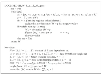
In this section, we propose a simple and fast algorithm DOOMRED that optimizes the base hypothesis weight set

W = {w1,. . .,wT}of f(x) in such a way to maximize the number of nontarget training instances whose margins are above a specificθvalue.Algorithm 1shows the pseudocode of DOOMRED. In [8], an algorithm named DOOM is introduced. DOOM optimizes the base hypothesis weight set W = {w1,. . .,wT} to minimize the cost function of the margins of the training instances. This optimization process results in the minimization of the classification error. However, DOOM cannot be directly applied to the detection problem. The reason is that basically DOOM is a two-class two-classification algorithm, and moreover it deals with the entire training instances of both classes in its optimization process. Since there are absolutely large amount of nontarget instances than that of target instances in rare-event detection problem, DOOM might show worse performance, especially low detection rate, when it is used for a rare-event detector. To solve this problem, we design the DOOMRED algorithm in which the target and the nontarget instances are dealt with separately in the optimization process.

DOOMRED is designed by adopting a simple steepest-gradient descent method. It is to guarantee the simplicity of the algorithm to minimize the computational burden for the optimization. Although DOOMRED only modifies the weights of the base hypotheses, there are great amount of training instances to deal with, which might result in a great amount of optimization time.

Before the optimization procedure, we need to define a marginal cost function to be minimized, that should be a monotonically decreasing function defined in the range from −1 to a specific θ value. The mean shifted sigmoid function in (13) and Figure 1 is an example. It represents the importance of each training instance during the optimization procedure:

Cθ(m)= 1

1 + expa×(m−(θ−1)/2), wherea >0. (13)

In DOOMRED, first, among the target and nontarget instances contained in the target training set SP and the nontarget training setSN, the instances whose margins are under the predefinedθPandθN are classified into the setsEP andEN, respectively. The training instances contained inEP andEN only aﬀect the modification of the base hypothesis weight set W. Then each base hypothesis weight wi ∈ W is modified to increase the margin of instances both inEP andEN.wiis increased if it decreases the summation of the marginal cost function Cθ(m) (cost (W)) of the instances inEPandEN, and vice versa. The amount of modification of wi is determined by the characteristic of the marginal cost function Cθ(m). For an example, when (13) is used as aCθ(m), instances whose margins are around (θ−1)/2 largely aﬀect the amount of modification ofwi. These two simple processes are iterated until cost (W) or variance ofW

converges. Note that DOOMRED may decrease the margins of the training instances which are not contained in the sets

Table 1: Parameter settings for the single layer optimization method inAlgorithm 2used in our experiments.

Parameter Value

Cθ(m) Figure 1(b)

NW 300

Variance ofθP 0.0 to 0.5 (step 0.1)

Variance ofθN 0.4 to 0.8 (step 0.1)

Prec 0.01

EP and EN. However, we also note from (2) that, after a certain value of θ is determined, the accuracy of f(x) is not aﬀected by the instances whose margins are aboveθ. It is because once θ is determined, the only issue we should consider is the portion of training instances whose margins exceed θ. After each DOOMRED execution, the threshold value is adjusted to make the training detection rate to be the specific goal value.

3.4. Single layer optimization method

Although we have derived a simple and clear optimization rule for a boosted single layer detector fromTheorem 1, one problem still remains that (2) does not provide the exact values of the key parameters to minimize the test error for the nontarget set. Since our objective is to find a globally optimal solution, DOOMRED is executed on the various randomly selected initial values of the base hypothesis weight setWR,

θP, andθN. Among these various trials,WSandθSwhich have the least false positive rate on the validation nontarget set

SNV are selected as the final output when the detection rate is fixed on the training target setSP. The final output of the optimization is a boosted detectorf(x) that is expressed with the originalH,W=WS, andθT=θS. The pseudocode of the single layer detector optimization is given inAlgorithm 2.

4. CASCADE DETECTOR OPTIMIZATION

For the optimization of a boosted cascade detector, the false-classified instances occurred in the real application are enforced to the first layer of the cascade detector. Then the optimization method for a single layer detector in

Algorithm 2is applied to each layer. In order not to degrade the eﬃciency of the cascade detector, the target and nontarget instances which are not rejected by any prelayer are used for the optimization of the postlayers.

5. EXPERIMENTAL RESULTS

5.1. Experimental environments

(8)

DOOMRED (H,W,SP,SN,θP,θN, prec)

exe=true while (exe)

EP=[(x,y)|(x,y)∈SP,y f(x)< θP],EN=[(x,y)|(x,y)∈SN,y f(x)< θN]

g= −∇Wcost (W)

if (W+ghas any negative valued element)

scalegthat no element ofW+ghas negative value if (weight Sum (g)≥prec)

WB=normalize (W+g)

if (cost (WB)<cost (W)) W=WB

else exe=false else exe=false returnW

Notations

H:= {hi|i=1,. . .,T}, number ofTbase hypotheses set

W:= {wi|i=1,. . .,T, 0< wi<1,Ti=1wi=1}, base hypothesis weight set

SP:= {(xi,yi)|xi=target training instance,yi=1}

SN := {(xi,yi)|xi=non-target training instance,yi= −1}

cost (W)=(xi,yi)∈EPCθP(yif(xi)) +

(xi,yi)∈ENCθN(yif(xi))

weight Sum (W)=T

i=1wi,wi∈W

normalize (W)=scaleWthatTi=1wi=1

Algorithm1: The pseudocode of DOOMRED.

instances among the second group by the completely trained detector are used as the enforced training data. The last group is used to measure the test errors.

Table 1shows the parameter settings for the optimization method used in the single layer detector in Algorithm 2. First, the digitized sigmoid function shown in Figure 1(b)

is defined asCθ(m). Since the exponential function requires large computational burden, the region from−1 to specific

θ is divided into 100 segments and the gradient of each segment is precomputed. Second, NW and the variation ranges ofθN andθPare set constant for all layers. These fixed values are determined by our tuning process. It might seem to be unreasonable to fixNWto be independent ofT, which is the number of the base hypotheses of f(x). However, for the boosted cascade detectors in most of real applications, no more than 200 base hypotheses are used to construct each single layer detector in the cascade detector. The number 300 for the random base hypothesis weight set is enough to make the performance of DOOMRED stable when the number of base hypothesis is under 200.

Experiments are performed on various boosted frontal face detectors trained using the Adaboost algorithm with diﬀerent conditions of the size of initial training set, base-hypotheses contained, and the enforced target training set. Note that since DOOMRED only modifies the weights of the base hypotheses, the performance of DOOMRED depends on the quality of the initial feature space constructed in the learning procedure.

The performance of DOOMRED is evaluated based on two criteria; (1) ROC curve, (2) optimization (or training) time. The first factor is critically related to the accuracy and the detection time in real applications. The second factor is related to the training or optimization cost of a detector. This

factor is particulary important since a boosting algorithm generally requires a large amount of training time. The performance of DOOMRED is compared to those of other heuristic solutions such as the adjusting threshold θT of single layer detector and retraining.

5.2. Experiments on single layer detectors

Figures 2, 3, and 4 show the ROC curves of various single layer detectors. InFigure 2, each original (or initial) detector was trained to have 200 base hypotheses. The face instances as many as 1000, 2000, 3000, and two times of each for the nonface instances were given as an initial training set. Then, false-rejected face instances which were not contained in the initial training set were enforced as many as 2000 false-classified nonface instances were enforced for the threshold adjusting and DOOMRED solutions, while 500 false-classified nonface instances were enforced for the retraining since the Adaboost algorithm occasionally failed to finish the learning procedure when 2000 nonface instances were enforced. In Figure 2, we can see that the amount of improvement in the accuracy by DOOMRED increased as the number of the initial training instance increased. Because DOOMRED deals with the weight set of base hypotheses only, the performance of DOOMRED seems to be aﬀected by the quality of the base hypotheses selected during the initial training process.

(9)

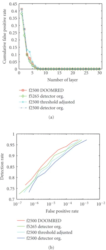
0 0.05 0.1 0.15 0.2 0.25 0.3 0.35 0.4 0.45

C

u

m

ulati

ve

false

p

ositi

ve

rat

e

0 5 10 15 20 25 30

Number of layer f2500 DOOMRED f5265 detector org. f2500 threshold adjusted f2500 detector org.

(a)

0.7 0.75 0.8 0.85 0.9 0.95 1

Det

ection

rat

e

10−7 ₁₀−6 ₁₀−5 ₁₀−4 ₁₀−3 ₁₀−2

False positive rate f2500 DOOMRED f5265 detector org. f2500 threshold adjusted f2500 detector org.

(b)

Figure6: (a) The false positive rates of the boosted cascade frontal face detectors before and after the optimization. (b) ROC curves of the boosted cascade frontal face detectors before and after the optimization estimated on CMU+MIT frontal face test images composed of 130 images containing 507 faces.

3, DOOMRED demonstrated stable and also remarkable performances compared with those of the other approaches. In the case when the number of the base hypotheses was 3, DOOMRED failed to increase the accuracy. This was because there were large amount of the face instances which were determined as −1 (nonface) by all the 3 base hypotheses. There was no chance for these faces to be determined as faces by only adjusting the weights of base hypotheses using DOOMRED.

InFigure 4, one initial detector was trained to have 200 base hypotheses with 2000 face and 4000 nonface instances. Then 10, 20, and 40 false-rejected face instances which were not contained in the initial training set were enforced. The size of the enforced nonface set were same as in Figure 2.

Table 2: The average number of the base hypotheses evaluated per each nonface instance and the optimization (or training) time estimated on Pentium 4 2.8 GHz PC.

Detector Average Optimization

num. of base hyp. Time(min)

F2500 org. detector 13.9 8291

F2500 doomred 17.6 704

F2500 thres adj. 20.3 4

F5265 org. detector 14.2 17431

It can be observed that DOOMRED increased the accuracy of the detectors when more enforced training instances were given. DOOMRED still showed stable and remarkable performance compared with those of the heuristic solutions. An interesting observation in our experiments was that the retraining sometimes failed to select 200 base hypotheses whose errors on the training set were under 0.5. A conclusion we can make on the single layer detector experiments is that DOOMRED exhibits a more stable and better performance than the other two naive approaches. The only exception was when the detector was initially trained with excessively small number of base hypotheses.

Figure 5shows the optimization (training) time for the tests in Figures 2, 3, and 4. DOOMRED required only less than 11.3% of the computation time for the retraining method, while showing similar or better test false positive rates as shown in Figures2,3, and4. Although the threshold adjusting method was fast by taking only a few minutes for any case, the performance was not satisfactory.

5.3. Experiments on cascade detectors

For this experiment, two boosted cascade frontal face detec-tors were initially constructed using AdaBoost algorithm. One was trained with an insuﬃcient number of training data including 2500 face and 5000 nonface instances, and it was composed of 30 layers (2500-face detector). The second cascade detector was trained with an abundant number of training data including 5265 face and 10530 nonface instances, and was composed of 30 layers (5265-face detector). Each cascade detector was constructed sequentially with one 3-base hypotheses, one 5-base hypotheses, three 20-base hypotheses, and two 50-base hypotheses layers. The number of base hypotheses of all the postlayers was set to 200. Then 431 false-rejected face instances which were not contained in the initial training set were enforced to the first layer of the 2500-face detector. Due to occasional failures in the learning procedure of the retraining solution as mentioned inSection 5.2, tests for the performance of the retraining method were substituted by that of the 5265-face detector. Note that the 5265-face detector may be considered as a detector retrained with 2500 initial faces and 2765 enforced faces.

(10)

OptimizeSingleLayer (H,SPI,SPE,SNI,SNE,DG, prec)

SP:=sumSPIandSPE,SN :=sumSNIandSNE

divideSNintoSNTandSNV

for (number ofNW)

WR=randomly generated base hypothesis weight set ofH

for (variousθPandθN)

WO=DOOMRED (H,WR,SP,SNT,θP,θN, prec)

adjustθTto getDGonSPwithH,WO

if (least false positive rate is made onSNVwithH,WO,θT)

WS=WO,θS=θT

returnWS,θS

Notations

H: base hypothesis set

SPI,SNI: initial target, non-target training set

SPE,SNE: enforced target, non-target training set

DG: goal detection rate of single layer detector

Algorithm2: The pseudocode for the optimization of the boosted single layer detector on the enforced training set.

at each single layer detector while showing good accuracy. As the 431 false-rejected faces were enforced to the 2500-face detector, the threshold adjusting method demonstrated good accuracy in the ROC curve even compared to that of the 5265-face detector as shown inFigure 6(b). We think that this is because the informative training instances (enforced training instances) eﬀectively compensated the distribution of the initial training set. However, one problem of this heuristic method is that the detector becomes slower in real applications as the number of the enforced instance increases. In Table 2, the average number of the base hypotheses calculated per nonface instance is shown, which is critically related to the detection time in real applications. When the thresholdθT of each layer was simply adjusted to acquire 99.5% of the training detection rate, the detection time increased by 46.0% and 42.9% compared to those of the 2500-face detector and 5265-face detectors. However, if DOOMRED was applied, these computational cost incre-ments decreased to 26.6% and 23.9% while showing the best accuracy among those of three other cases in Figure 6(b). Note also that the optimization time of DOOMRED on the 2500-face detector was 704 minutes as shown inTable 2. This is barely 8.5% and 4.0% of the training time required in the 2500-face detector and 5265-face detectors, respectively. Therefore, we can conclude that the proposed DOOMRED is a reasonable solution for the optimization of the boosted cascade detector on the enforced training set considering its excellent performance to enhance the detection speed and accuracy in reasonable optimization time.

6. CONCLUSION

In this paper, we proposed DOOMRED, an algorithm to modify the base hypothesis weight set initially constructed by a boosting algorithm. It can be applied to the boosted single layer or cascade detector when the false-classified training

set is enforced. Experimental results demonstrated that DOOMRED excellently enhanced the performance of the boosted single layer or cascade detectors compared to those of other heuristic approaches while requiring reasonable optimization time. DOOMRED, however, showed weak per-formance when the number of the base hypotheses is small. To overcome this limitation, we are planning to develop an eﬃcient algorithm that can substitute the inappropriate base hypotheses with the optimal ones.

ACKNOWLEDGMENT

This work was supported in part by the ITRC program by Ministry of Information and Communication and in part by Defense Acquisition Program Administration and Agency for Defense Development, South Korea, through the Image Information Research Center under the Contract UD070007AD.

REFERENCES

[1] P. Viola and M. Jones, “Rapid object detection using a boosted cascade of simple features,” inProceedings of the IEEE Computer Society Conference on Computer Vision and Pattern Recognition

(CVPR ’01), vol. 1, pp. 511–518, Kauai, Hawaii, USA, December

2001.

[2] A. Demiriz, K. P. Bennett, and J. Shawe-Taylor, “Linear pro-gramming boosting via column generation,”Machine Learning, vol. 46, no. 1–3, pp. 225–254, 2002.

[3] S. Z. Li and Z. Zhang, “FloatBoost learning and statistical face detection,”IEEE Transactions on Pattern Analysis and Machine

Intelligence, vol. 26, no. 9, pp. 1112–1123, 2004.

[4] P. Viola and M. Jones, “Fast and robust classification using asymmetric adaboost and a detector cascade,” inAdvances in

Neural Information Processing Systems 14, pp. 1311–1318, MIT

(11)

[5] T. J. Hastie and R. J. Tibshirani,Generalized Additive Models, Chapman & Hall/CRC, London, UK, 1990.

[6] R. E. Schapire, Y. Freund, P. L. Bartlett, and W. S. Lee, “Boosting the margin: a new explanation for the eﬀectiveness of voting methods,”The Annals of Statistics, vol. 26, no. 5, pp. 1651–1686, 1998.

[7] Y. Freund and R. E. Schapire, “A decision-theoretic generaliza-tion of on-line learning and an applicageneraliza-tion to boosting,”Journal

of Computer and System Sciences, vol. 55, no. 1, pp. 119–139,

1997.