Formal Methods for Control Synthesis in Partially Observed Environments: Application to Autonomous Robotic Manipulation

(1)

Formal Methods for Control Synthesis in Partially Observed

Environments: Application to Autonomous Robotic

Manipulation

Thesis by

Rangoli Sharan

In Partial Fulfillment of the Requirements for the Degree of

Doctor of Philosophy

California Institute of Technology Pasadena, California

2014

(2)

(3)

Acknowledgements

I owe my deepest gratitude to my advisor, Professor Joel Burdick, for his support and guidance throughout my Ph.D. studies. In addition to providing crucial insight and direction for the com-pletion of this research, his encouragement to pursue my own interests is greatly appreciated. I have been very fortunate to have Joel’s unreserved understanding – in pursuing my own research problem of interest, exploring opportunities outside the PhD program, and the challenges of my long distance marriage. He has greatly shaped my values and attitude towards work and life. I am also thankful to have had the opportunity to work on the DARPA ARM-S challenge at the Jet Propulsion Laboratory (JPL). My time there was not only a great learning opportunity, but also provided the main motivation for this work.

It has been a great pleasure to have Professor Richard Murray as a mentor. It has been a won-derful experience to interact frequently with him. The research presented in this thesis is greatly inspired by the work that he and his students are actively developing. It has been eye-opening to see the process of developing fundamental theoretical results and the eﬀort to bring together col-laborators from other academic institutions and partners from the industry to move new knowledge into crucial application areas.

I am honored to have Professor Jim Beck on my thesis committee. Some of the research during my early Ph.D. years utilized Bayesian inference algorithms, to which I was first exposed in a class taught by Professor Beck. To him I owe new lenses with which I view many technical problems that I face in daily life or find worthy to solve for the world at large.

Some of my happiest workdays have been at JPL working with Dr. Nicolas Hudson on the DARPA ARM-S challenge. While my research was peripheral to the team’s success in the compe-tition, I always found myself welcome to his limited time and the resources of his lab. It is a great pleasure to have him on my thesis committee.

I want to acknowledge the wonderful experience with the whole team at JPL: Paul Hebert, Jeremy Ma, Max Bajracharya, and especially Dr. Paul Backes who was extremely supportive and facilitated my work at JPL.

(4)

My friends and colleagues from the Burdick and Murray groups: Tom, Melissa, Matanya, Kr-ishna, Jeﬀ, Eric, Scott and Vasu; and my roommates for various lengths of time: Piya and Na, have inspired me with their relentless pursuit of deeper understanding and also provided much needed light moments during the workdays.

I am fortunate to have enjoyed the unconditional friendship of Sushree and Jaykrishnan. They provided a much needed support structure in Pasadena. The tea breaks and home-cooked meals shared together are some of my fondest memories during the years at Caltech. My closest friends – Anjali, Jyoti, Romila, Shruti and Vertika – have stood by me through every personal and professional upheaval of the last decade. They are a never-ending source of joy and support.

Finally, I want to acknowledge the incredible support I receive everyday from my family. My parents, Shashi and Rita, have dedicated their lives and sacrificed greatly to support their two children in any and all endeavors. I can only hope to navigate life’s challenges with their perseverance and foresight. My brother Anand, who has always been my safety net, and his wife Nidhi, bring laughter and joy everyday. I take this opportunity to especially remember my late grandfather Vaidehi, my earliest academic mentor, to whom I owe my apetite for learning and problem solving. I am extremely fortunate to have found new sources of love and support in Pramila, Toshita, Vaibhav, Svana, and Shwetank, great new additions to my family, that occured during my PhD years.

(5)

Abstract

Modern robots are increasingly expected to function in uncertain and dynamically challenging en-vironments, often in proximity with humans. In addition, wide scale adoption of robots requires on-the-fly adaptability of software for diverse application. These requirements strongly suggest the need to adopt formal representations of high level goals and safety specifications, especially as tem-poral logic formulas. This approach allows for the use of formal verification techniques for controller synthesis that can give guarantees for safety and performance. Robots operating in unstructured environments also face limited sensing capability. Correctly inferring a robot’s progress toward high level goal can be challenging.

This thesis develops new algorithms for synthesizing discrete controllers in partially known en-vironments under specifications represented as linear temporal logic (LTL) formulas. It is inspired by recent developments in finite abstraction techniques for hybrid systems and motion planning problems. The robot and its environment is assumed to have a finite abstraction as a Partially Observable Markov Decision Process (POMDP), which is a powerful model class capable of repre-senting a wide variety of problems. However, synthesizing controllers that satisfy LTL goals over POMDPs is a challenging problem which has received only limited attention.

This thesis proposes tractable, approximate algorithms for the control synthesis problem using

Finite State Controllers (FSCs). The use of FSCs to control finite POMDPs allows for the closed system to be analyzed as finite global Markov chain. The thesis explicitly shows how transient and steady state behavior of the global Markov chains can be related to two diﬀerent criteria with respect to satisfaction of LTL formulas. First, the maximization of the probability of LTL satisfaction is related to an optimization problem over a parametrization of the FSC. Analytic computation of gradients are derived which allows the use of first order optimization techniques.

The second criterion encourages rapid and frequent visits to a restricted set of states over infinite executions. It is formulated as a constrained optimization problem with a discounted long term reward objective by the novel utilization of a fundamental equation for Markov chains - the Poisson equation. A new constrained policy iteration technique is proposed to solve the resulting dynamic program, which also provides a way to escape local maxima.

(6)

(7)

List of Figures

1.1 The DARPA ARM-S Robot . . . 3

2.1 Graphical representation of the DRA translations of common LTL specifications. . . . 14

2.2 Partially observable probabilistic grid world . . . 16

2.3 Evolution of a labeled POMDP. . . 17

3.1 POMDP controlled by an FSC . . . 27

3.2 Eﬀect of FSC structure onϕ-feasibility . . . 40

4.1 Logistic function . . . 44

4.2 RepeatP Mϕ can be visited with vanishing frequency. . . 54

4.3 Generating Admissible Structures of FSC . . . 58

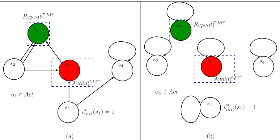
4.4 System Models for Case Study I. . . 62

4.5 DRA for the LTL specificationϕ1“˝♦a^˝♦b^␣c . . . 63

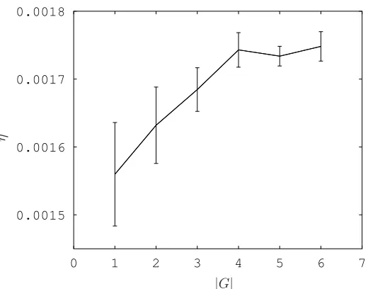
4.6 Dependence of expected steady state average rewardη on size of FSC . . . 64

4.7 System Model for Case Study II . . . 65

4.8 Sample trajectories under optimal controllers . . . 66

5.1 Assigning rewards for visitingRepeatP Mϕ frequently. . . 70

5.2 ModifyingTϕ _{for steady state}_ϕ_{-feasibility. . . .} ₇₂

5.3 Example where visitingAvoidP Mϕ is required to reachRepeatP Mϕ . . . 73

5.4 Steady state detecting global Markov chain. . . 76

5.5 Steady state detecting global Markov chain. . . 77

5.6 Reduced Feasibility arising from Conservative Optimization Criterion . . . 79

6.1 Value Function for a two state POMDP . . . 87

6.2 Eﬀect of DP Backup Equation . . . 90

6.3 Eﬀect of I-state Improvement LP . . . 93

6.4 Policy Iteration Local Maximum . . . 93

(13)

6.6 Transient behavior optimization using Bounded Policy Iteration . . . 106

6.7 Eﬀect of Bounded Policy Iteration on steady state behavior. . . 107

7.1 Various Robotic Paradigms . . . 111

7.2 A Hybrid Robot Architecture . . . 114

7.3 The DARPA ARM-S Robot. . . 117

7.4 Wheel Removal Task for the ARM-S Robot . . . 118

7.5 Abstracted digraph for removing nuts with impact driver. . . 121

7.6 Execution for remanipulation task of Example 2 . . . 132

7.7 Probabilistic Outcomes and Partial Observability in ARM-S . . . 133

7.8 DRA for ARM-S Tasks . . . 134

7.9 DBN of the ARM-S task planning domain. . . 135

7.10 Bounded Policy Iteration for ARM Task 1 . . . 136

7.11 Bounded Policy Iteration for ARM Task 2 . . . 137

(14)

List of Tables

3.1 Complexity of LTL satisfaction over POMDPs . . . 32

4.1 Results for GW-B underϕ2 . . . 65

4.2 Finding the Initial Feasible Controller by Algorithm 4.2. . . 67

7.1 Problem size of policy iteration for naive implementation. . . 128

(15)

List of Algorithms

4.1 Generate Set To Visit Frequently . . . 54

4.2 Generate Candidate FSCs . . . 59

6.1 Policy Iteration for Markov Decision Process . . . 85

6.2 Bounded PI: Adding I-States to Escape Local Maxima . . . 94

6.3 Bounded Policy Iteration For Conservative Optimization Criterion . . . 96

6.4 Adding I-states to Escape Local Maxima of Constrained Optimization Criterion . . . 102

6.5 Pruning candidate successor I-states and actions to satisfy recurrence constraints. . . 103

7.1 A common compound task . . . 120

(16)

Chapter 1

Introduction

1.1

Motivation

Robots and autonomous control systems are regularly required to function in uncertain and dy-namically changing environments. They are also increasingly required to satisfy complex sets of rules that specify desired system behavior. These requirements are often specified in addition to the traditional control theoretic goals, e.g., set point or trajectory tracking, stability margins, re-sponse time, etc. Such complex goal satisfaction requirements arise in diverse areas like aerospace, energy management systems, robotics, civic and transportation planning, resource and supply chain management, autonomous vehicles and manufacturing. Many of these application areas also employ numerous, possibly distributed, sensors and actuators.

Autonomous platforms such as self-driving cars and unmanned aerial vehicles (UAVs) are now being deployed in the commercial, military, and public domains. The success of these platforms are crucially dependent on their safe operability and ability to adapt to continuously evolving local laws. This presents the challenge of verifying the control and sensing algorithms against safety and abstract rules, and synthesizing new controllers if required.

This work is motivated by the challenges faced by autonomous robots deployed in unstructured environments. A particular motivation is the need of such robots to manipulate objects in their environment through the use of articulated limbs. Applications for such robots are numerous, some examples being

• Personal Robotics: Robots that are capable of manipulating made-for-human objects to pro-vide assistance at home and in the oﬃce. Of special interest are robots that can assist the disabled or elderly.

(17)

which damaged areas could not be accessed safely by humans due to nuclear radiation. • Security and Defense: Applications in security and defense include searching for IEDs in

luggage, vehicles or on persons at checkpoints, which requires dextrous manipulation in un-structured and unknown environments, or in reconnaissance.

In particular, this thesis tackles a few of the challenges that were faced by the Caltech/JPL team during the DARPA Autonomous Robotic Manipulation - Software (ARM-S) challenge [3]. This challenge, which focused on autonomous robotic manipulation of real-world objects during complex tasks in semi-structured environments, is described in detail in Chapter 7. For example, one challenge task involved the use of a two-armed robot to replace a tire attached to an immobile hub, as shown in Figure 1.1. A typical process to remove the wheel might include the following sequence: the robot locates and acquires an impact driver, grasps the driver so that it can properly depress the power trigger, positions the driver on the lug nuts, removes the nuts one by one, puts down the impact driver so that both hands are free, and removes the wheel. The robot faces many hurdles during this process. Since the tool and tire manipulation tasks are kinematically linked, the robot may pick up the impact driver in a pose where the lug nuts can be removed, but the driver trigger cannot be depressed. Second, sensor-based operations, such as localization of objects, are noisy, which may result in failure at the task level. Worse still, it may be impossible to determine if some subtasks were executed correctly, e.g. visual or force-torque sensors may be incapable of determining precisely whether the lug nuts were successfully removed. It is currently diﬃcult to program such tasks at a high level of abstraction, and to guarantee some level of performance.

Two main problems arise in the context of complex manipulation tasks requiring a sequence of actions. First, the free configuration space, Cf ree, [91, 92] can have high dimension and a complex representation due to the presence of multiple manipulator joints and numerous objects, commonly referred to as configuration space obstacles,CO. The dimension and complexity are further exacer-bated because these obstacles can be moved, and attached to/detached from other obstacles or the end eﬀector by grasping or placing objects. Furthermore, the attachment can be any of a variety of rigid or non-rigid configurations. These characteristics imply a “hybrid” planning problem. The movement of the end eﬀector inCf ree whenCOis unchanging is a path planning planning problem in continuous space, whereas the process of grasping and attachment of objects introduces discrete changes to the definition of CO and the topology of Cf ree - a problem which and falls under the purview of task planning.

(18)

(19)

manipulator in such a way that changes in CO only occur at the end of any local control task. However, since the outcome of the local control execution cannot be guaranteed, nor can the change in CO be observed accurately, the task level plan must incorporate the execution explicitly, i.e., it must describe how to interpret sensor observations to determine the next local controller to deploy. Instead of tackling the problem of autonomous manipulation planning and its control and exe-cution in their full hybrid dynamical system domain, this thesis focuses exclusively on planning over finite discrete choices. The imperfect control and sensing encountered at the continuous low level controllers are assumed to be abstracted to obtain a finite discrete model by the introduction of uncertainty in the discrete motion model and by incorporating partial observability of the discrete states.

Additionally, this work focuses on synthesizing a control policy for goals or specifications that can be expressed in a formal language. Specifically, these specifications will be expressed as formulas belonging to the class of propositional logic calledLinear Temporal Logic. Linear Temporal Logic oﬀers a rich set of temporal specifications or properties that the controlled system can be verified against. The key benefit of these specifications is that they allow verification of properties overpaths

taken by the controlled system rather than properties of the goal state alone. For example, for a robot on an assembly line shared with humans, it may be required that the robot halts all motion when a human is within a specified distance of its workspace, and then resumes its trajectory to a goal state when the human recedes. Another example of a temporal and logical specification over the robot’s trajectory is the requirement to reach multiple goal states in a specified order.

1.2

Related Work

Validation and verification form two aspects of testing a software or hardware system’s fitness for its intended purpose. While validation is concerned with generating or designing specifications as per need, verification is concerned with checking if the system design or implementation satisfies those specifications. In computer science and control theory, formal methods from mathematics are used extensively for specification, design, implementation and verification of software and hardware systems. Formal verification is concerned with proving or disproving whether the algorithms will behave properly with respect to the specifications. Software systems are usually modeled as discrete state and discrete time, and typical specifications are concerned with avoiding deadlocks and live-locks in concurrent systems, or ensuring safety, reachability and liveness conditions in more general settings. The specifications are usually in the form of temporal logics such as Linear Temporal Logic (LTL) or Computational Tree Logic (CTL).

(20)

finite models. Pioneering work in model checking formalisms can be found in [36, 43, 125]. Model checking suﬀers from the curse of dimensionality: even a small symbolic representation of either the specifications or the underlying system, can result in very large intermediate state spaces which the model checker must explore. However, this has been mitigated recently in two ways. Recently, a large and expressive subset of temporal logic specifications were shown to have solutions with only polynomial time complexity [114]. Additionally, several techniques in symbolic model checking allow sets of states to be explored simultaneously, circumventing explicit state enumeration. These methodologies include Binary Decision Diagrams [26], model abstraction and counterexample based refinement [37] and partial order reduction [48,111,142]. The work presented in this thesis takes the model checking approach to formal verification.

The second approach is deductive verification. In this approach, the system model and the specifications are used to generate a set of proof obligations. The burden is then on automated or interactive theorem provers to establish the truth of these proof obligations. Deductive verification is based on the framework found in [45, 58]. The initial introduction of temporal logic for specifi-cation and verifispecifi-cation of concurrent systems also relied on theorem proving [116, 117]. While this methodology allows for infinite state space models, often skilled interaction between the designer and the proof system is required, an approach which is diﬃcult to scale to large systems.

In typical control design problems, the physical systems are usually not exclusively discrete. For systems governed by diﬀerential equations, Lyapunov based techniques and reachability analysis provide methods to design controllers that satisfy safety, reachability and stability criteria. However, many complex controlled autonomous systems are hybrid in nature, e.g. robots, aircraft, climate control, energy management systems, etc. The hybrid nature arises due to the complex digital software, abstraction of mixed signal circuits, switches, etc. A survey of formal verification techniques for hybrid systems can be found in [2].

Recently, formal methods have become increasing popular in robotics [40, 76–78, 148], where simultaneous motion and task planning is a challenging problem. In [40, 140] the authors synthesize controllers that give probabilistic guarantees of temporal logic specifications in discrete systems. In [68] take a sampling based approach to carry out motion planning by incrementally building discrete abstractions that satisfy local formal specifications. In [146], the authors demonstrate a receding horizon approach by decomposing a high level specification into several components – generation of a sequence of short term goals, trajectory planning and continuous controller design – while provably satisfying the overall specification. In [151], the authors demonstrate how game theoretic methods can be employed to carry out multi-robot motion planning.

(21)

checking methods for control synthesis can be found in [75]. In [14], the authors abstract polygonal environments into a discrete model to synthesize controllers for temporal logic specifications. In [35], a noisy continuous state system is approximated as a finite MDP to satisfy various classes of temporal logics. The main idea is that the discrete abstraction is carried out by computing both the continuous state reachability properties and the invariance of the discrete states or high level properties. This ensures that a high level, discrete plan is guaranteed to be realizable by a series of continuous controllers [147, 148]. For cases when the environment is only partially known a-priori, on-line iterative and backtracking frameworks for formal control synthesis have also been proposed [87, 95]. Moreover, in [88], the authors propose techniques for locally patching the control strategy if parts of the original strategy are invalidated due to change in environment or incorrect assumptions.

Numerous practical applications of formal methods in robotics have been demonstrated. In [34] the authors demonstrate the applicability of these methods in dextrous manipulation tasks focusing on finger-gaiting. Similarly, model checking has been employed in autonomous vehicles [4, 121] and to specify emergent behaviors in swarm robotics [143].

It is also important to note the contributions from research in the area of domain independent planning, as robot task planning is a key application for the algorithms developed in that area. Traditionally, domain independent planning concerned itself with planning exclusively in the discrete and deterministic domain – e.g. problems representable in STRIPS-like representation scheme. Classical planning problems could also be exclusively characterized as reachability problems – the solution from the planning algorithm would provide a sequence of actions that can lead to a goal state from the initial state. However, domain independent planning has grown to include almost all of robot motion and task planning challenges in its purview – temporal goal satisfaction, timed actions, preference based action selection, probabilistic and partially observable domains, continuous states, etc. A bibliographic overview of task planning from a domain independent perspective is provided in Chapter 7.

In robotics, Linear Temporal Logic (LTL) is a popular choice for robot goal and safety specifi-cation as it is a powerful and expressive class of temporal logic with intuitive correlation to natural language [59,104]. Notably, LTL formulas can represent goals over infinite executions. This is useful for representing persistent surveillance and applications where robots are always online. In order to capture environmental disturbance, it is often useful to model the dynamics as a probabilistic system. Markov decision processes are a popular choice for the discrete abstraction of noisy sys-tems. In the case of (fully observable) Markov decision process (MDP), synthesis of controllers with probabilistic satisfaction guarantees of LTL specification is well understood [8]. In fact, for fully observable MDPs under LTL specifications, robust [144] and receding horizon controllers [146] have been formulated.

(22)

strategies EXPTIME-completeness of a broad set of objectives (parity objectives) is proven in [32]. In a recent publication [33], the existence and construction of finite memory strategy for (strictly) positive probability of satisfaction is shown to be an EXPTIME-complete problem. The memory requirements for a controller that guarantees satisfaction with probability 1 are established to be exponential as well. In [145], the authors discretize the belief space, which is the set of all probability distributions over the state space, a-priori. Then the resulting discrete model is a fully observable MDP for which formal control synthesis is well established. However, for POMDPs aa-priori belief space discretization can be suboptimal and prohibitive for large state spaces. In this thesis, a goal centric approach is taken – the controller has discrete states and optimizes the input to the controlled system and its own dynamics for each state according to the LTL specification. Such class of controllers is known to implicitly partition the belief space of the controlled system into sets of regions – each corresponding to a discrete controller state.

1.3

Thesis Overview and Contributions

The objective of this thesis is to provide tractable algorithms for synthesis of control systems which satisfy Linear Temporal Logic specifications in a partially observable setting. Specifically, the thesis will take a model based approach – the robot and environment will be modeled as a finite, discrete time Partially Observable Markov Decision Process. The motivating application consists of combined task planning and execution in autonomous systems with imperfect sensing and control.

Chapter 2 provides the formalization and background of the problem domain. It introduces Lin-ear Temporal Logic (LTL) in the context of a general state transition system, and the methodology of verifying LTL formulas by constructing an automaton. It also formalizes the model that is used to abstract the controlled system of interest. The system is assumed to be modeled as a finite Partially Observable Markov Decision Process (POMDP). The chapter also provides a brief overview of the classical problems and solution approaches for this class of model.

(23)

Chapter 4 begins by introducing the notion of thestructureandquality of an FSC. It then shows how to solve the problem of maximizing the probability of satisfying an LTL formula when the structure of the FSC is fixed, and the controller transition and action choices are parametrized. The problem is formulated as a nonlinear optimization problem and gradient computations are derived analytically to allow the use of first order optimization methods. Gradient based methods have been used for reward maximization problems over POMDPs. However, this thesis presents a new explicit formulation for gradient based optimization of LTL satisfaction probability in which there is no a-priori reward associated with states and actions of the controlled system. Case studies are presented at the end of this chapter to demonstrate some key aspects and limitations of these algorithm. A preliminary version of the work in this chapter of the thesis also appears in [131].

Chapter 5 deviates from the problem of maximizing LTL satisfactionprobability explicitly. The main focus is to derive a reward scheme that drives the solution of the LTL satisfaction problem to rapid convergence to a steady state behavior in which certain states are visited often while others are avoided with probability 1. The notion of rewardingfrequent visits to “good” states of the state space is introduced via discounting. Discounting not only ensures rapid convergence to steady state, but also frequent visits to “good” statesduring steady state system execution, setting it apart from the gradient based algorithm of Chapter 4. While having the practical importance of causing the controlled system to visit goal states sooner and frequently, the decision to use discounting is also motivated by the convergence properties and existence of eﬃcient dynamic programming algorithms. The proposed reward schemes are completely new to the best of my knowledge. However, the reward scheme and the resulting optimization problems proposed in this thesis form sound, but not complete algorithms for maximization of LTL satisfaction probability over POMDPs.

Chapter 6 proposes a Policy Iteration algorithm to solve the optimization problem introduced in the preceding chapter. Some key aspects relating to this algorithm is that it oﬀers a way to search directly over both the structure and the quality of the FSC. This overcomes the limitation of the gradient method of Chapter 4 which did not oﬀer a way to choose the size or structure of the FSC. Moreover, the FSC transitions and action choices are no longer parametrized, but directly computed as a result of the optimization. The proposed algorithm is based on the bounded policy iteration algorithm proposed in [118] and [54]. However, the use of the Poisson Equation for Markov chains as a constraint to avoid certain states in steady state and its solution is entirely new to the best of my knowledge.

(24)

for integrating a task level planner during execution for the system. The example task of removing a wheel from a fixed hub, introduced earlier in this chapter, is formalized using a recently introduced planning domain description language and two case studies of LTL satisfaction for the ARM-S robot are carried out.

(25)

Chapter 2

Background

This chapter provides background for the rest of the thesis. First, an overview of Linear Temporal Logic, its representation using automata, and typical temporal properties in control are described. Next, finite partially observable Markov decision processes (POMDPs) are formally reviewed. Fi-nally, classical problems in this domain and typical solution methods are described.

2.1

Linear Temporal Logic

Temporal logic is a branch of logic that enables representation and reasoning about temporal aspects of a system [8,42,65]. It deals with propositions qualified in terms of time, e.g., “The train isalways

on time.” It was introduced first astense logicin [119]. Since its first use as a specification language by Pnueli in [96], temporal logic has been demonstrated to be especially suited to reason about concurrent programs. Is has been utilized to formally specify and verify behavior in a variety of applications [30, 38, 46, 60, 66, 86, 115, 148].

In this thesis, a subset of temporal logic, namely linear temporal logic (LTL) is considered. Before formally defining LTL, a brief overview of the underlying building blocks for LTL is provided. The notation in this section closely follows that of [148].

Definition 2.1.1 Asystemconsists of a setV of variables. ThedomainofV, denoted by dompVq, is the set of valuations ofV. Astateof the system is an elementvPdompVq.

Definition 2.1.2 An atomic proposition is a statement p on system variables v P V that has a unique truth value (T rueorF alse) for a given statev. LetvPdompVqbe a state of the system and pbe an atomic proposition. Writingv,psignifies thatpisT rueat the state v. Otherwise v.p.

(26)

LTL is a propositional logic built inductively from logical connectives and temporal modal oper-ators. The logical connectives are the familiar operators: negation ␣,disjunction_,conjunction^, and implication ùñ . The temporal operators includealways l, eventually ♦, next l, anduntil

U.

Syntax: An LTL formula is defined inductively as follows:

1. any atomic propositionpis an atomic formula; and

2. given LTL formulasϕandψ, the expressions␣ϕ,ϕ_ψ,lϕ,ϕU ψ are LTL formulas. Other formulas can be defined in terms of the above as follows:

• ϕ^ψfi␣p␣ϕ_ψq, • ϕ ùñ ψfi␣ϕ_ψ, • ♦ϕfiT rueU ϕ, and • lϕfi␣♦␣ϕ.

Semantics: An LTL formula is interpreted over an infinite sequence of states. Given an exe-cutionσ“v0v1v2. . . and an LTL formulaϕ, it is said thatϕholds at position tě0 ofσ, written

vt ( ϕ, if and only if (iﬀ) ϕ holds for the remainder of the execution σ starting at position i. Formally, the semantics of LTL is defined inductively as follows.

• For an atomic proposition p,vt(piﬀvt,p, • vt(␣ϕiﬀvt*ϕ,

• vt(ϕ_ψiﬀvt(ϕorvt(ψ, • vt( lϕiﬀvt`1(ϕ, and

• vt(ϕU ψ iﬀDt1ět such thatvt1 (ψand@t2P rt, t1q, v_t2 (ϕ.

Thus the temporal operators are thus interpreted as follows: lϕholds at position t of σ iﬀϕ

holds at the next statet`1,lϕholds at positiontiﬀϕholds at every position ofσstart at position

t, and ♦ϕholds at positiont iﬀϕholds at some positiont1 ět inσ.

(27)

2.1.1

Verification of LTL satisfaction using Automata

From the previous section, it is clear that an LTL formulaϕdefines a set of infinite executions. In order to verify and synthesize controllers that enable the system to satisfyϕ, the aim is to construct an automaton which accepts only those infinite executions [8]. It is well known that for any LTL formulaϕover a set of atomic propositionsAP, one can construct adeterministic Rabin automaton

(DRA), with the input alphabet 2AP_{, that accepts all and only those infinite words that satisfy the}

LTL formula [49,73,141]. Algorithms for converting LTL formulas to DRAs can be found in [74,141], and a common free software tool to carry out the conversion is at [72].

Definition 2.1.4 A deterministic Rabin automaton (DRA) is a five-tuple A “ pQ,Σ,δ, q0,Ωq,

where

• Q is the set of states;

• Σis the input alphabet. In the context of atomic propositions over a system, Σ“2AP_.

• δ:QˆΣÑQis the deterministic transition function.

• q0PQis the initial state.

• Ω “ tpAvoidr, Repeatrq|r P t1, . . . , NΩu, Avoidr, Repeatr Ď Su is the Rabin acceptance condition.

Definition 2.1.5 (Rabin Acceptance) A runπ“q0q1. . . of a DRAAwith acceptance condition

Ω “ tpAvoid1, Repeatiq, . . .pAvoidN_Ω, RepeatN_Ωqu is accepting if there exists an r P t1, . . . , NΩu

such thatInfpπq XAvoidr“ HandInfpπq XRepeatr‰ H. HereInfpπqare the set of states that occur infinitely often inπ.

Stated otherwise, the Rabin acceptance conditions mean that for some pairpAvoidr, Repeatrq P

Ω, no state inAvoidris visited infinitely often, while some state inRepeatris visited infinitely often. The DRA is used for verification of an LTL formulaϕas follows. It is assumed that the interesting properties of the system are given by a set of atomic propositions AP over the variables V of the system. An executionσ“v0v1. . . of the system therefore leads to a unique (infinite)trace over the truth evaluations ofAP, given byhpσqfihpv0qhpv1q. . .. Herehpvtq P2AP simply denotes the truth

value of all atomic propositions inAP at time step tusing the statevt. At the start of the system

(28)

2.1.2

Common LTL formulas in Control

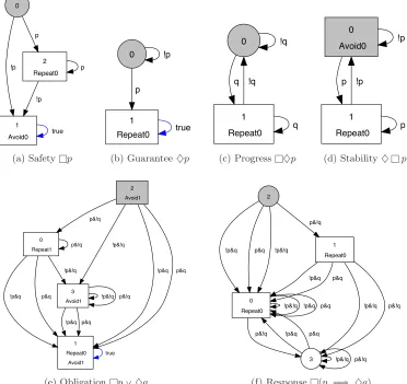
There are a few LTL formulas that arise naturally for controlled systems, denoting the typical goals of control system design. A list of these typical formulas, along with a graphical representation of their corresponding deterministic Rabin automaton, is provided below. The translation to automaton representation was carried out using the software tools described in [72] and [61].

2.1.2.1 Safety or Invariance

A safety or invariance formula, Fig. 2.1(a), is of the form lp, wherepis an atomic proposition or LTL formula. It asserts that the propertypremains invariant throughout an execution. Invariance is used to specify the requirement that something bad never happens. For example, for a wheeled robot, “Never be close to a staircase” can ensure operation safety.

2.1.2.2 Guarantee or Reachability

A guarantee formula, Fig. 2.1(b), is of the form♦p. It specifies that the propositionpwill eventually become true during the execution. It denotes that something good is guaranteed to occur, or some goal state will be reached by the system.

2.1.2.3 Progress or Recurrence

A progress property, Fig. 2.1(c), is given by l♦p. It ensures that the propertypholds infinitely often during execution. It essentially ensures that some good property will always be achieved.

2.1.2.4 Stability or Persistence

A stability property, Fig. 2.1(d) given by♦lp, ensures that after a transient period, a propertyp

becomes true andthen remains invariant for the rest of the execution. This is similar to the notion of stability in classical control, in which the system is steered towards an operating point and the control must ensure that it operates close to, or at, this operating point.

2.1.2.5 Obligation

The obligation property, Fig. 2.1(e), given bylp_♦q, is a disjunction of invariance and guarantee. Thus, it ensures that either some reachability goal is met or some invariant property always holds.

2.1.2.6 Response

(29)

0 1 Avoid0 2 Repeat0 !p p true !p p 0 1 Repeat0 !p p true 0 1 Repeat0 !q

q !q

q 0 Avoid0 1 Repeat0 !p

p !p

p

(a) Safetylp (b) Guarantee♦p (c) Progressl♦p (d) Stability♦lp

0 Repeat1 3 Avoid1 1 Repeat0 Avoid1 2 Avoid1 p&!q !p&!q

!p&q p&q !p&!q p&!q

!p&q p&q

true p&!q

!p&!q

!p&q p&q

0 Repeat0 3 1 Repeat0 2

!p&!q !p&q p&q

p&!q !p&q p&q

!p&!q p&!q !p&q p&q

!p&!q p&!q !p&q p&q !p&!q

p&!q

(e) Obligationlp_♦q (f) Responselpp ùñ ♦qq

Figure 2.1: Graphical representation of the DRA translations of common LTL specifications. The states of the DRA are given by the nodes (circles or boxes) and are numbered. The gray nodes denote start state of the DRA. The deterministic transitions are marked by the truth evaluations ofAP. Square nodes belong to some numbered Rabin acceptance condition pair pRepeat0, Avoid0q, . . .. Note that in the DRA for Obligation specification in (e), the node 1

(30)

2.2

Labeled Partially Observable Markov Decision Process

Definition 2.2.1 (Labeled-POMDP) Formally, a labeled-POMDP,PMconsists of:

• |Smodel_|_states_Smodel_{“ t}_smodel

1 , . . . , smodel_|S_model_|uof the world,

• |Act|actions or controls Act“ tα1, . . . ,α_|Act|uavailable to the reactive agent, • |O|observations O“ to1, . . . , o_|O|u,

• |AP| atomic propositionsAP “ tp1, p2, . . . p_|AP|u.

• Possibly a reward, rpsmodel

i q PR, for each statesmodeli PSmodel.

This thesis assumes that the POMDPs are finite, in which Smodel_, _Act_, _{O, and} _AP _{are finite}

sets. Each action α P Act determines the probability of making a transition from some state

smodel_i P Smodel _{to state} _smodel

j PSmodel given byTpsmodelj |smodeli ,αq. Additionally, for each state

smodel

i , an observation o P O is generated independently with probability Opo|smodeli q. It is also

assumed that the probability that the start state of the world issmodel

i is given by the distribution

ιinitpsmodeli q. The probabilistic components of a POMDP model must satisfy the following:

ÿ

smodel_PSmodel

Tpsmodel|smodel_i ,αq “1 @smodel_i PSmodel,αPAct

ÿ

oPO

Opo|smodelq “1 @smodelPSmodel

ÿ

smodel_PSmodel

ιinitpsmodelq “1.

Finally, for each state smodel_i , a labeling function hpsmodel_i q P 2AP _{assigns the truth value to}

all the atomic propositions in AP in each state. Note that, the truth valuation of propositions in

AP can in general be both a function of state and action, and can even be stochastic. For ease of exposition, this work exclusively focuses on state dependent deterministic propositions.

While in general, rewards may be a function of both the state and the action taken by an agent, it is assumed that rewards are a function of the state only, and are awarded once during state transition. To state this formally, if the world state transitions fromsmodel

i tosmodelj , then rewardrpsmodelj qis

issued. The initial state,smodel_p_t_“_{0q, of the world also gathers the reward}_r_p_smodel_p_t_“_0qq.

While this restriction of the rewards to a function of state is not required, this reward scheme will be suﬃcient for synthesizing controllers that satisfy LTL formulas over POMDPs.

The final restriction is that the world model is assumed to be time invariant, i.e.,Smodel_, _Act_,

(31)

1 2 4 5 6

7 8 9 10

3

13

b a

R

11 12

0

M=7 N

R

0.1

0.1 0.8

c

0.8 0.1

0.1

1.0 0.05

0.05 0.05

0.05 0.05 0.05

0.6

start

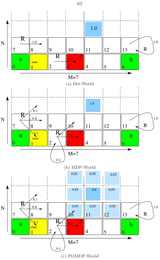
Figure 2.2: Partially observable probabilistic grid world. It is described in example 2.2.2.

Example 2.2.2 (GridWorld-A) An example whose variants will be used repeatedly to demon-strate various aspects of the problem requirements and solution methodology is the labeled-POMDP represented in Fig. 2.2. It represents a grid world of size M ˆN, with fixed M “7 and varying

N ě1 in which a robot can move from cell to cell. Thus the state space is given by

S“ tpsi|i“x`M y, xP t0, . . . , M´1u, yP t0, . . . , N´1uu.

The action set available to the robot is

Act“ tRight, Lef t, U p, Down, Stopu.

The actionsRight, Lef t, U pandDown, cause probabilistic motion of the robot from its current cell to a neighboring cell. The probabilities for the state transitions for various types of cell (near a wall, or interior) are shown for actionRightin the figure.Lef t, U p, andDownhave symmetric definitions. The action Stopis deterministic, in which the robot stays in its current cell. Partial observability arises because the robot does not precisely know its cell location. It can take measurements to ascertain it. The observation space is given by

O“ toi|i“x`M y, xP t0, . . . , M´1u, yP t0, . . . , N´1uu.

Given the actual cell position (dark blue) of the robot, the location measurement has a distribution over the actual position and nearby cells (light blue). Cell 1 in yellow shows the initial state of the robot. Thus,

ιinitps1q “1.

(32)

are three atomic propositions of interest in this world, giving

AP “ ta, b, cu.

In cell 0,ais true, whilebandcare true in cells 6 and 3 respectively.

Definition 2.2.3 (Path in a POMDP) An infinitepathin a (labeled) POMDP,PM, with states sPS is an infinite sequenceπ“s0o0α1s1o1α2¨ ¨ ¨ P pSˆOˆActqω, such that@tě0

Tpst`1|st,αt`1qą0, Opot|stqą0, and

ιinitps0qą0.

Any finite prefix of πthat ends in either a state or an observation is a finite path fragment.

Pictorially, the process evolves as in Fig. 2.3. Even though the underlying states at each time step are not fully observable, the model is assumed to start at some states0. Associated with each statest, an observationotis emitted according toO and is available to the agent. Since the labels

hp.qare tied to the state, the labelinghpstqis also partially observed at any time stept. Subsequently an action at`1 causes the state of the world to evolve from st tost`1. Note that since no method for choosing actions has been introduced until now, the actionsαi are non-deterministic.

s0 s1 s2

α1 α2

o0, hps0q o1, hps1q o2, hps2q

Figure 2.3: Evolution of a labeled POMDP.

The above formulation has minor diﬀerences from common formulations in literature, which assume that the first observation is availableafter the first action is applied. This is diﬀerent from Figure 2.3, where the first action occurs after receiving an observation from the world, which can be used to further refine the initial distributionιinit. Thus, if there is an agent that chooses actions,

(33)

2.2.1

Information State Process (ISP) induced by the POMDP

Let It denote all information available until time step t. Since at any step the action taken and the observation received are the only two new quantities known to an agent,It`1“ rIt,αt`1, ot`1s.

This leads to the following information state process (ISP)I“ tI0, I1, . . .u:

I0 “ rιinit, o0s

I1 “ rI0,α1, o1s

I2 “ rI1,α2, o2s ..

.

The domain of the ISPI can be defined inductively

dompI0q “ MSˆO

dompItq “ dompIt´1q ˆActˆO

so that the overall domain is

dompIq “ď

t

dompItq

In the above, MS is the set of all distributions over S. In the context of transition systems, distributions are sometimes thought of as beliefs over the states S, signifying the likelihood of actually being in diﬀerent states at a given time step.

The formal definition of a distribution and its derivation from probability measures is discussed in appendix A.

2.2.2

Belief State Process (BSP) induced by the POMDP

Clearly, the representation of the ISP in computer memory requires an exponentially bounded (p|Act||O|t_{) amount of space. Instead, a popular method of modeling the process to keep track}

(34)

b0psq “ řιinitpsqOpo0|sq

oPO

ιinitpsqOpo|sq

(2.1)

btpsq “ 1

cOpot|s,αtq

ÿ

s1_PS

Tps|s1,αtqbt´1ps1q, tě1 (2.2)

wherecis a normalizing constant given by

c“ ÿ

sPS

Opot|s,αtq

ÿ

sPS

Tps|s1,αtqbt´1ps1q, tě1.

Equation 2.2 is called the belief update equation. In fact, the belief state process (BSP) B “ tb0, b1, . . .uforms a continuous state space (fully observable) Markov decision process, evolving in the space of all distributionsMS as defined in Section 2.2.1. At any time step t, the belief statebt

can be computed from the information stateItinductively.

2.2.3

POMDP controllers

From the definition of a (labeled) POMDP, and the associated ISP or BSP, it is unclear how actions at each time step are chosen. This is the task of theagent, used interchangeably with thecontroller

orscheduler. The controller chooses the actionsαt using apolicy which formalizes the rules used to

decide actions using some or all information available to the controller up to the current time step. Typically, policies are categorized into deterministic and stochastic policies.

Definition 2.2.4 (Deterministic Policy) Let PM be a POMDP, and its ISP given by I. A

deterministic policyfor PM, denotedµis function

µ:dompIq ÑAct (2.3)

Definition 2.2.5 (Stochastic Policy) LetPMbe a POMDP, and its ISP given byI. A stochas-tic policyfor PM, denoted µis a function

µ:dompIq ÑMAct (2.4)

whereMAct is the set of all probability distributions over the naturalσ´algebra over Act.

For deterministic policies, actions are directly determined asαt“µtfiµpIt´1q. For stochastic

policiesµpIt´1qis a distribution that must be sampled independently to generate the actionαtand

this should be written asαt„µt“µpIt´1q. However, the equalityαt“µtwill be used to represent

(35)

Most importantly, the outcome of this definition of a policy is that the ISPI “ tI0, I1, . . .uis Markovian.

2.2.3.1 Markov Chain Induced by a Policy

Given a POMDPPMwith state spaceS, at´step execution is given by

σ0:t“s0s1. . . stPSloooomoooonˆ. . .S

t`1 times

“St`1 (2.5)

Then the processMµ_S`“ tσ0:0,σ0:1, . . .uevolves stochastically in the space

S`“

8

ď

t“0

St`1. (2.6)

The initial probability distribution is given by

Prrσ0:0s “b0ps0q, (2.7)

and the state transition probabilities are given by

Tpσ0:_t`1|σo:tq “Tpst`1|st, µpItqq. (2.8)

Since It itself is Markovian, the processMµ_S` forms a Markov chain. However, this Markov chain has infinite state space,S`_{. In Section 3.1.1, it will be shown that a class of controllers leads to a}

Markov chain over a finite state space that is equivalent toMµ_S`.

2.2.4

Probability Space over Markov Chains

LetMbe a Markov chain over a countable set of statesS. Let the initial state distribution be given by ιinitpsq, sPS and the state transition probability given by Tpsj|siq. In this work, the notion

of probability of events in a Markov chain is used extensively. It is therefore necessary to formally define the probability space associated with M. A detailed description can be found in [8] from where the following definitions are borrowed. A brief primer on probability measures is provided in appendix A. Three quantities are of interest to fully specify a probability spacepX,F, µq, whereX

is the underlying set of outcomes, F Ď2X _{is a} _σ_{´algebra over} _X _and _µ _{is a probability measure}

over the sets in F. For infinite executions of Markov chains, i.e., t Ñ 8, each of these is defined next.

(36)

Definition 2.2.6 (Paths of a Markov chain) Define as P athspMq the set of all infinite se-quences π “ s0s1¨ ¨ ¨ P Sω, such that @t ě 0, Tpst`1|stq ą 0 and ιinitps0q ą 0. In addition, also define the set of all finite path fragments P athsf inpMq “ tprefixpπq|πP P athspMqu, i.e., by collecting all finite prefixes from every infinite pathπPP athspMq.

Next, in order to specify the σ´algebra,F, of concern, define the cylinder sets of the Markov chain as follows.

Definition 2.2.7 (Cylinder Set) The cylinder setofˆπ“s0s1. . . sn PP athsf inpMqis defined as

Cylpˆπq “ tπPP athspMq |πˆ P pref ixpπqu. (2.9)

In other words, the cylinder set spanned by finite path fragment ˆπis the set of all infinite paths that start with ˆπ. Next, denote the set of all possible cylinder sets asCY L. Formally

CY L“ tCylpˆπq|ˆπPP athsf inpMqu. (2.10)

Clearly, CY L P 2X_{. As stated in Section A.5, there exists a (unique) smallest} _σ_{´algebra that}

containsCY L, denotedσpCY Lq. This gives theF“σpCY Lq, where thebasis events are given by

Cylpˆπq.

Finally, in order to specify the probability measure over all the sets or events in F “σpCY Lq, it is suﬃcient to provide the probability of each cylinder set inCY L. This is computed as

PrMrCylps0. . . snqs “ιinitps0q

ź

0_ďtăn

Tpst`1|stq. (2.11)

Once the probability measure is defined over the cylinder sets, the expectation operator EM is

also uniquely defined from its definition. In the sequel, if the underlying Markov chain is clear from context, the subscript will be dropped and Pr andEwill be used.

2.2.5

Typical Problems over POMDPs

In a typical POMDP control problem, states are assumed to issue rewards as the agent influences the world to visit various states. For a finite execution σ0:T “s0s1. . . sT, the cumulative reward

received by the agent is given byřT_t“0rptq. Another quantity of interest is the average reward per time step _T1řT_t“0rptqespecially whenT Ñ 8. Many problems also assume that good events visited early in the execution are better. In order to incentivize temporal greediness, the accumulated reward is formulated as the discounted sumřT_t“0βtrptq, with 0ăβă1.

(37)

quantities of interest are maximized inexpectation.

Two main maximization objectives are of interest in this work, and are studied widely in litera-ture.

Definition 2.2.8 (Total Expected Discounted Reward) For a finite horizon or time stepsT, this criterion is given by

ηβpTq “EMµ

« _T

ÿ

t“0

βtrptq

ˇ ˇ ˇ ˇ

ˇιinit

ﬀ

, for 0ăβ ă1, (2.12)

whereβ is the discount factor. For infinite horizon, the criterion is given by the limit

ηβ“ lim

TÑ8EMµ

« _T

ÿ

t“0

βtrptq

ˇ ˇ ˇ ˇ

ˇιinit

ﬀ

, for 0ăβă1. (2.13)

Definition 2.2.9 (Expected Average Reward) For a finite horizon or time stepsT, this crite-rion is given by

ηavpTq “EMµ

« 1 T T ÿ t“0

rptq

ˇ ˇ ˇ ˇ

ˇιinit

ﬀ

. (2.14)

For infinite horizon, the criterion is given by the limit

ηav“ lim

TÑ8EMµ

« 1 T T ÿ t“0

rptq

ˇ ˇ ˇ ˇ

ˇιinit

ﬀ

. (2.15)

Let η be one of the above criteria; then the optimization problem of interest in the classical POMDP control setting is

maximize

µ η. (2.16)

2.2.6

Optimal and

ϵ

´optimal Policy

Assume that an optimal valueη˚ of a given objective from the various reward criteria exists. Then any policy µ˚ that attains this optimum is called an optimal policy. Let ηµ _{be the value of the}

objective under some known policyµ. For anyϵą0,µis calledϵ-optimal if

η˚ěηµěη˚´ϵ, (2.17)

thus signifying that the value of the objective is at mostϵbelow the optimal value under the policy

(38)

2.2.7

Brief overview of solution methods

The solution methods for typical POMDP problems fall under two categories: exact and approxi-mate. A detailed survey is found in the introductory chapters of [1], and in [24]. These are briefly summarized here.

2.2.7.1 Exact Methods

Exact methods typically need to employ the full information stateIt to design the policy. However this requires infinite memory as t Ñ 8 and is intractable. As has already been mentioned, the belief state bt oﬀers a suﬃcient statistic for It . Following [29, 137], the problem is solved using

Dynamic Programming [16] over a belief space MDP that can be constructed from a POMDP. However, since the belief state space is uncountably infinite, these algorithms may require infinite memory for representation. Also the complexity of these algorithms grows exponentially with the size of the state space, and hence it is diﬃcult to solve problems with more than a few tens of states, observations and actions.

2.2.7.2 Approximate Methods

In recent years, there has been a lot of work in approximating the value function. For example, one method is to assume that the underlying system is an MDP and learning the underlying Q-function and employing heuristics such as the most likely state heuristic, the voting heuristic,QM DP-heuristic, or exploiting the entropy of the belief state [67,106,135]. Another is to use grid based methods [22,55]. Other approximate methods search only over the reachable belief states and fall under point-based POMDP planning [79,113]. The algorithms in this thesis also utilize an approximate method because they search exclusively in the space of policies that require finite internal memory. This particular controller, called a Finite State Controller is introduced in detail in the next chapter in Section 3.1.

2.3

Concluding Remarks

(39)

(40)

Chapter 3

LTL Satisfaction using Finite State

Controllers

In the previous chapter, the POMDP and its associated problems in the form of optimization ob-jectives were introduced. Further, the various methods of designing controllers to maximize these criteria were mentioned. In this chapter, one particular class of controllers, called the finite state controller is studied in detail. The choice of this class of controllers is shown to lead to a finite state space Markov chain for the closed loop controlled system. This allows easy analysis of infinite executions of the system in the context of satisfying an LTL formula of interest. Next, the various categories of problems relating to LTL formulas over POMDPs controlled by FSCs are formalized. Finally, a brief overview of the solution methodology for these problems is provided.

It is a well known fact that POMDP, and for some criteria, MDP controllers require memory or internal states [1,29,67]. Let the controller’s internal states be denoted bygPG“ tg1, g2, . . . , g_|G|u.

Finite state controllers have finite |G|. As mentioned before, infinite horizon problems typically require infinite|G|. The most popular method that employs infinite memory design controllers that work in the belief space which is continuous, which eﬀectively implies uncountably infiniteG. For this case the above definition does not hold.

Finite state controllers are formally defined next.

3.1

Finite State Controllers

Definition 3.1.1 (Deterministic Finite State Controller (det-FSC)) LetPMbe a POMDP with observation setO, action setActand initial distributionιinit as in Definition 2.2.1s. A

deter-ministic finite state controller (det-FSC) for PMis given by the tupleG“ pG,ω,κqwhere

• G“ tg1, g2, . . . , g_|G|uis a finite set of internal states.

(41)

apply to PM.

• κ:MS ÑGchooses the start state g0“κpιinitq, of the FSC given initial distributionιinit.

Definition 3.1.2 (Stochastic Finite State Controller (sto-FSC)) LetPMbe a POMDP with observation set O, action set Act and initial distribution ιinit. A stochastic finite state controller

(sto-FSC)for PMis given by the tupleG“ pG,ω,κqwhere

• G“ tg1, g2, . . . , g_|G|uis a finite set of internal states.

• ω :GˆO ÑMGˆAct is a function such that given a current internal state of FSC, gk and

observation o,ωpgk, oqis a probability distribution over GˆAct. The next internal state and action pair pgl,αq are chosen by independent sampling of ωpgk, oq. By abuse of notation, we will useωpgl,α|gk, oqas the probability of transitioning to I-stategland taking actionα, when the current I-state isgk and observation received is o.

• κ:MS ÑMGchooses the starting internal stateg0, by independent sampling ofκpιinitq, given initial distribution ιinit of PM. Again, by abuse of notation, we will use κpg|ιinitqto denote the probability of starting the FSC in internal state g when the initial distribution is given by

ιinit.

Any deterministic FSC can be written as a special case of stochastic FSCs. This thesis will exclusively consider the stochastic version and so the term FSC will denote a stochastic FSC unless otherwise stated.

A schematic diagram of how an FSC controls the POMDP is shown in Figure 3.1. Under the FSC, the POMDP evolves as follows.

1. Sett“0. POMDP initial states0is initialized by drawing independently from the distribution

ιinit. The deterministic or stochastic functionκpιinitqis used to determine or sample the initial

FSC I-stateg0.

2. At each time step tě 0, the POMDP emits an observationot according to the distribution Op.|stq.

3. The FSC determines its new stategt`1and actionαt`1according to the deterministic function or stochastic distribution given byωp.|gt, otq.

4. The actionαt`1is applied to the POMDP, which transitions to a new statest`1 according to the distribution Tp.|st,αq.

(42)

POMDP

ω α

gk gl

o

FSC

Figure 3.1: POMDP controlled by an FSC

3.1.1

Markov Chain induced by an FSC

Closing the loop around a POMDP with an FSC, as in Figure 3.1, yields the following transition system.

Definition 3.1.3 (Global Markov Chain) Let S be the state space of the POMDP,PM, andG be the set of I-states of the FSC, G, as in Definition 3.1.2. The global Markov chain MP M,GSˆG with

execution σ“ trs0, g0s,rs1, g1s, . . .u, rst, gts PSˆGevolves as follows:

• The probability of the initial global staters0, g0sis given by

ιP M,G_init rrs0, g0ss “ιinitps0qκpg0|ιinitq (3.1)

• The state transition probability is given by

TP M,Grrst`1, gt`1s |rst, gts s “

ÿ

oPO

ÿ

αPAct

Opo|stqωpgt`1,α|gt, oqTpst`1|st,αq (3.2)

Note that for a finite state space POMDP, the global Markov chain has finite state space. Similar to the fully observable case of Markov decision process in [8], the global Markov chain induced by the finite state controller MP M,G_SˆG is probabilistically bisimilar to the infinite state space Markov chain described in Section 2.2.3.1. Probabilistic bisimilarity is discussed in [8, 80].

(43)

3.2

LTL satisfaction over POMDP executions

This section formalizes how infinite traces obtained from POMDP executions can be verified against an LTL formula ϕ. This is carried out by constructing the product of the labeled POMDP,PM, and the DRA obtained from translatingϕ.

Definition 3.2.1 (Product-POMDP) LetPMbe a labeled POMDP (Definition 2.2.1) with state spaceSmodel_{, actions}_{Act, observations}_O_{, atomic propositions}_AP_{, transition probabilities}_T_p_._|_s,_α_q_:

SÑ r0,1s, @smodel_P_Smodel_,_α_P_{Act, and labeling function} _h_:_Smodel_Ñ₂AP_.

Next, let the LTL formula ϕ be translated to the deterministic Rabin automaton (Definition 2.1.4), denoted Aϕ_{, with state space} _{Q, initial state} _q

0, input alphabet 2AP, transition function

δ : Qˆ2AP _Ñ _Q _{and with} _Ω _{“ p}_{Repeati, Avoidi}_q _{s.t. Repeati} _Ď _{Q, Avoidi} _Ď _{Q, the Rabin} acceptance condition.

The product-POMDP denoted PMϕ is a POMDP with state space S “Smodel_ˆ_{Q, the same} action set Actand observations O.

• The transition probabilities of PMϕ are given by

Tϕ`s1 “ xsmodel_j , qly|s“ xsmodel_i , qky,α˘“

$ & %

Tpsmodel

j |smodeli ,αq ifδpqk, hpsmodeli qq “ql

0 otherwise.

(3.3) • The initial state probability distribution is given by

ιϕ_init`s“ xsmodel, qy˘“

$ & %

ιinitpsmodelq ifδpq0, hpsmodelqq “q

0 otherwise.

(3.4)

• The observation probabilities are

Oϕpo|s“ xsmodel, qyq “Opo|smodelq. (3.5)

• If rewards rpsmodelqare defined over the original modelPM, then we define new rewards over the product states are defined as

rϕps“ xsmodel, qyq “rpsmodelq. (3.6)

In addition, using the Rabin acceptance pairs Ω from Aϕ_{, we also define the accepting pairs}

ΩP Mϕ _{“ tp}_RepeatP Mϕ

i , AvoidP M

ϕ

(44)

states“ xsmodel_{, q}_y _of _PMϕ _{is in}_RepeatP Mϕ

i iﬀ qPRepeati ands“ xsmodel, qy is inAvoidP M

ϕ

i

iﬀ qPAvoidi. Note that|ΩP Mϕ_{| “ |}_Ω_|_.

3.2.1

Inducing an FSC for

PM

from that of

PM

ϕ

The product POMDP is the basis for a method to find a policy as defined by an FSC. However, the resulting policy is meant to be applied to the Product-POMDP. However the goal is to control the original POMDP,PMand it is necessary to formally define how to derive a policy for PMfrom a policy computed forPMϕ.

Note that in the case of fully observable MDPs, the choice of action as a function of the current state of the Product-POMDP is usually suﬃcient [8]. In this case a policyα“µps“ xsmodel_{, q}_yq_for

the product-MDP induces the policy for the original MDP by settingα“µmodel_p_smodel_{q “} _µ_p_s_“

xsmodel_{, q}_yq_{at each time step [40].}

In the case of POMDPs, given the internal state of the controller, the only new information at each time step is the most recent action and observation. These action and observation sets remain unchanged between the original model PM and the product-POMDP PMϕ. However, the start state of the FSC is determined by the initial distribution of the product-POMDP.

Definition 3.2.2 (Inducing an FSC) Let G “ pG,κ,ωq be the FSC that controls the product-POMDP PMϕ. The FSC Gmodel _{“ p}_Gmodel_,_κmodel_,_ωmodel_q _{that controls the original POMDP}

PMis induced as follows.

• The internal nodes of Gmodel _{are the same as that of} _G_{. That is,}_Gmodel_“_G.

• Let κpιϕ_initq be the distribution that determines the initial node of G. Then the initial node of

Gmodel _{is given by setting}

κmodelpιinitq “κpιϕinitq. (3.7)

• The probability of transitioning between I-states and issuing an action αis obtained by

ωmodelpgl,α|gk, oq “ωpgl,α|gk, oq, @oPO,αPAct,and gk, glPG“Gmodel. (3.8)

3.2.2

Verification of LTL Satisfaction using Product-POMDP

Now let’s consider the criterion for an (infinite) execution ofPMto satisfyϕ. Letσϕ“s0s1. . . , st“

xsmodel

(45)

Definition 3.2.3 (Accepting execution) We say thatσϕ _{is an} _{accepting execution} _{if, for some}

pRepeatP Mϕ

i , AvoidP M

ϕ

i q P ΩP M

ϕ

such that σϕ _{intersects with} _RepeatP Mϕ

i infinitely often, while

it intersects withAvoidP M_i ϕ only a finite number of times.

The notion of verifying LTL properties using product transition systems in well known in the literature [8, 40] and the following lemma is stated without a formal proof.

Lemma 3.2.4 Let σϕ _“ _s

0s1. . . , withst “ xsmodelt , qty be an execution of PMϕ and the corre-sponding execution of PMbe given