Volume 2006, Article ID 59625, Pages1–17 DOI 10.1155/ASP/2006/59625
Microphone Array Speaker Localizers Using
Spatial-Temporal Information
Sharon Gannot1and Tsvi Gregory Dvorkind2
1School of Engineering, Bar-Ilan University, Ramat-Gan 52900, Israel
2Department of Electrical Engineering, Technion – Israel Institute of Technology, Technion City, Haifa 32000, Israel
Received 20 January 2005; Revised 17 May 2005; Accepted 22 August 2005
A dual-step approach for speaker localization based on a microphone array is addressed in this paper. In the first stage, which is not the main concern of this paper, the time difference between arrivals of the speech signal at each pair of microphones is estimated. These readings are combined in the second stage to obtain the source location. In this paper, we focus on the second stage of the localization task. In this contribution, we propose to exploit the speaker’s smooth trajectory for improving the current position estimate. Three localization schemes, which use the temporal information, are presented. The first is a recursive form of the Gauss method. The other two are extensions of the Kalman filter to the nonlinear problem at hand, namely, theextended Kalman filterand theunscented Kalman filter. These methods are compared with other algorithms, which do not make use of the temporal information. An extensive experimental study demonstrates the advantage of using the spatial-temporal methods. To gain some insight on the obtainable performance of the localization algorithm, an approximate analytical evaluation, verified by an experimental study, is conducted. This study shows that in common TDOA-based localization scenarios—where the microphone array has small interelement spread relative to the source position—the elevation and azimuth angles can be accurately estimated, whereas the Cartesian coordinates as well as the range are poorly estimated.
Copyright © 2006 Hindawi Publishing Corporation. All rights reserved.
1. INTRODUCTION AND PROBLEM FORMULATION
Determining the spatial position of a speaker finds a grow-ing interest in video conference scenarios where automated camera steering and tracking are required. Acoustic source localization might also be used as a preprocessor stage for speech enhancement algorithms, which are based on micro-phone array beamformers.
Usually, methods for speaker localization are comprised of two stages. In the first stage, which is not the main con-cern of this paper, microphone array is used for extracting
the time difference between arrivals of the speech signal at
each pair of microphones. These readings are then processed by the second stage to obtain the source position. This pa-per focus is on the second algorithmic stage of the two-step approaches.
In the first algorithmic stage, the time difference of
ar-rival (TDOA) is estimated using spatially separated micro-phone pairs. The classical method for performing this task is
the generalized cross-correlation (GCC) algorithm [1]. Many
improvements of this method for the reverberant case exist. Brandstein and Silverman used a robust estimate of the
cross-power spectral density phase [2]. A cepstrum-based prefilter
applied to the received signals prior to the application of the
cross-correlation is proven by St´ephene and Champagne to
be beneficial [3]. Benesty [4] and Doclo and Moonen [5] are
using subspace tracking methods for performing the
desig-nated task. Recently, Dvorkind and Gannot [6–8] proposed a
method for TDOA estimation, based on the nonstationarity of the speech signal, which was proven to be superior to the other methods in tracking scenarios.
During the second algorithmic stage, the noisy TDOA readings are combined to produce the source location esti-mate. The locus of speaker positions associated with a given microphone pair, from which we have extracted a TDOA measurement, forms one half of a hyperboloid of two sheets. By intersecting hyperboloid surfaces, one can estimate the
speaker position [9]. However, this formulation is hard to
compute in 3-dimensional space and tends to be noise sensi-tive (since small measurement errors can divert the intersec-tion curve significantly). Another approach is useful in far-field applications, where the hyperboloid is approximated by a cone (centered at the midpoint of the microphone pair). By intersecting the bearing lines associated with such cones, location estimate can be derived by properly weighting the potential source locations according to the likelihood of the
measurement. Brandstein et al. denote this method bylinear
By manipulating the measurement model, as will be shown in the sequel, the hyperbolic equations can be recast into a spherical form. The obtained equation set is shown to be nonlinear. Since the number of equations increases with the number of microphones, the noisy case can be solved by applying the (nonlinear) least squares (LS) approach.
The nonlinear LS problem yields a cumbersome
expres-sion. This difficulty might be alleviated in several ways. Three
methods provide a closed-form solution, which differ in the
way they mitigate the nonlinearity. Thespherical intersection
(SX) method was proposed by Schau and Robinson [11]. The
spherical interpolation (SI) was proposed by Smith and Abel
[12], while Huang et al. proposed theone-step least squares
(OSLS) method [13]. Dealing with the differences between
these methods is beyond the scope of this short survey.
Recently, Huang et al. [14] addressed the same
nonlin-ear equation set and solved it by using Lagrange multiplier. Since a polynomial of degree six is involved in the proposed method, no closed-form solution exists. Thus, the iterative
secant method [15] was used for the root search. The
two-step approach is referred to as linear correction least squares (LCLS) approach. We will elaborate more on this method while formulating the problem.
Direct maximum likelihood-based algorithms are widely used in the localization task. Maximum likelihood (ML) pro-cessors require a priori knowledge of the joint probabil-ity densprobabil-ity function of the errors in the TDOAs, and need search-based algorithms for determining the maximizer. Yao
et al. [16] proposed a frequency-domain, one-step,
approx-imate ML estimator for extracting both the source location and the received signal spectrum. They also proposed an it-erative method for dealing with multiple source scenarios. Chen et al. further developed this concept and presented the Cram´er-Rao lower bound (CRLB) for the localization
prob-lem in [17]. When the microphones locations are not known
exactly, a two-stage estimation procedure is proposed, where iterations are performed between the ML estimation stage and a calibration stage. In the ML context, Segal et al. work should be mentioned, in which the estimate-maximize (EM) procedure is applied (in the frequency domain) for estimat-ing both the position of several sources and their respective
parameters [18]. Birchfield and Gillmor [19] utilized Bayes
rule to obtain an ML estimator for the source location. In a simplified, reverberant-free room, the proposed method is shown to be more robust against additive noise than the
conventional beamformer. Chen et al. [17] proposed the
use of two beamformers with several look directions for ex-tracting several candidate azimuth angles. A majority-based rule is then used for estimating the azimuth angle of the source.
All the prementioned methods exploit the spatial
in-formation obtained by different microphone pairs, but do
not exploit the temporal information available from adjoint speaker position estimates. The speaker smooth trajectory can be used to obtain a more robust localization estimate. Bayesian estimation procedures were previously proposed by
Ward et al. [20] and Vermaak and Blake [21]. In the former,
a particle filter is used in conjunction with a beamformer to
Mici
Mic mi
Mic0
mj
Micj φs(t)
θs(t) s(t)
Speech source
Di
Figure1: Microphone array. Speaker location at time instanttis
s(t) with azimuth angleφs(t) and elevation angleθs(t). Microphone
position notated bymi;i=0,. . .,M.
estimate the speaker position in a one-stage procedure. In the latter, the reverberation model is considered through a bimodal distribution of the noisy measurement around the true TDOA. Utilizing this distribution and giving a first-order Markov process model for the speaker trajectory, a par-ticle filter is derived and applied to the problem at hand.
Lehmann and Williamson [22] also used the particle
fil-ter. However they incorporate the importance sampling (IS) concept, in which particles are generated in each time step, based on the previous time step and the current measure-ment. The importance function is implemented based on a
delay-and-sum beamforming results. Bechler et al. [23]
pro-posed the use of a two-stage algorithm. In the first, the TDOA
readings are used by the OSLS method [13] to obtain an
initial estimate of the speaker position. These estimates are spatially smoothed by using three parallel linear Kalman
fil-ters. Each of the filters is using a different state transition
model, namely, static, constant velocity, and constant accel-eration. The three Kalman filters are weighted according to their a posteriori probability given the measurements. Klee
and McDonough [24] showed by simulation results that the
intermediate stage, in which source is localized by the SX method before applying the Kalman filter, deteriorates the
overall performance. They proposed instead to apply the
it-erated extended Kalman filter directly on the TDOA read-ings.
In [25] we introduced two methods for exploiting the
speaker’s smooth trajectory for improving the tracking abil-ity of source localizers, namely, a recursive Gauss (RG) method and the extended Kalman filter (EKF). These meth-ods were compared with several nontemporal methmeth-ods. In
[26] the use of the unscented Kalman filter (UKF) for the
problem at hand was proposed. The current contribution,
which is an extension of the ideas presented in both [7,26],
includes a more detailed exposition of the ideas and a com-prehensive comparative experimental study.
We turn now to an exact formulation of the localization
problem. Consider anM+ 1 microphones array as depicted
coordinates mi [xi yi zi]T; i = 0,. . .,M. To simplify
the exposition, the location of a reference microphone m0
is set as the axes originm0 =[0 0 0]T. (·)T stands for the
transpose operation. Define the source coordinates at time
instanttbys(t)[xs(t) ys(t) zs(t)]T. Each of theM
mi-crophones, combined with the reference microphone, is used
at time instanttto extract a TDOA measurementτi(t);i =
1,. . .,M [8]. Denote theith range difference measurement
byri(t)=cτi(t), wherecis the sound propagation speed
(ap-proximately 340 m/s in air). It can be easily verified from
sim-ple geometrical considerations (seeFigure 1) that this range
difference is related to the source and the microphone
loca-tion by the nonlinear equaloca-tion
ri(t)=s(t)−mi−s(t), i=1,. . .,M, (1)
where the fact that the reference microphone is positioned at the origin was used.
Usually, only an estimate of the real TDOA is available.
Thus, concatenating M estimates of the quantity in (1), a
nonlinear measurement model is obtained:
r(t)=
⎡ ⎢ ⎢ ⎢ ⎣
s(t)−m1−s(t)
.. .
s(t)−mM−s(t)
⎤ ⎥ ⎥ ⎥
⎦+v(t)h
s(t)+v(t).
(2)
Here,vT(t)=[v1(t) v2(t) · · · vM(t)] is a vector of
mea-surement errors, depicting the nonperfect estimate of the
range differences. The goal of the localization task is to
ex-tract the speaker’s trajectory s(t) from the measurements
vectorr(t). Any estimation procedure (e.g., [1,4,5] or [8])
could be used for the TDOA estimation. The methods intro-duced in this contribution, constituting the second stage of the localization procedure, are independent of the choice of the first stage.
Following the derivation presented in [11–14], a practical
approach for solving the nonlinear problem can be derived.
Defining the distance between the speaker and theith
micro-phone asDi(t)s(t)−mi(seeFigure 1), we get
D2
i(t)=s(t)−mi2=s(t)2−2mTis(t) +mi2. (3)
However, using (1), the estimated distance is given by
Di(t)=ri(t) +s(t), i=1,. . .,M. (4)
An estimator of the speaker location is derived by minimiz-ing the error between the estimated and the true squared
distance:
i(t)12 D2i(t)−D2i(t)
=mTis(t) +ri(t)s(t)
−1
2
mi2−r2i(t)
, i=1,. . .,M. (5)
Concatenating the equations in (5), we have
(t)=A(t)gs(t)−b(t), (6)
where
A(t) ⎡ ⎢ ⎢ ⎢ ⎢ ⎢ ⎢ ⎣
x1 y1 z1 r1(t)
x2 y2 z2 r2(t)
.. . xM yM zM rM(t)
⎤ ⎥ ⎥ ⎥ ⎥ ⎥ ⎥ ⎦ ,
b(t) 1 2 ⎡ ⎢ ⎢ ⎢ ⎢ ⎢ ⎢ ⎢ ⎣
m12
−r2 1(t)
m22
−r2 2(t)
.. .
mM2
−r2
M(t)
⎤ ⎥ ⎥ ⎥ ⎥ ⎥ ⎥ ⎥ ⎦ ,
gs(t) ⎡ ⎢ ⎢ ⎢ ⎢ ⎣
xs(t) ys(t) zs(t)
s(t)
⎤ ⎥ ⎥ ⎥ ⎥
⎦, (t)
⎡ ⎢ ⎢ ⎢ ⎢ ⎢ ⎢ ⎣
1(t)
2(t)
.. . M(t)
⎤ ⎥ ⎥ ⎥ ⎥ ⎥ ⎥ ⎦ . (7)
The estimation problem is thus converted into a
minimiza-tion problem of the quantityT(t)(t) with respect to the
nonlinear functionalg(s(t)). Since the fourth component of
the vectorg(s(t)) is related to the first three, the
minimiza-tion problem becomes a constrained LS problem.
In [14] this problem was solved by using theLagrange
multiplierstechnique yielding
gs(t)=AT(t)A(t) +λΣ−1
AT(t)b(t), (8)
where Σ diag[1 1 1 −1]1 andλ is the Lagrange
mul-tiplier, imposing the (quadratic) constraint ong(s(t))
struc-ture. It can be shown thatλis obtained by finding the roots of
a polynomial of degree six. Due to the complexity of the poly-nomial equation, numerical methods for root finding should
be used. Therefore it is proposed in [14] to first solve the
unconstrained LS problem and then use a linear correction
1We denote by diag(m
1,m2,. . .) a diagonal matrix withm1,m2,. . .on its
in the second phase. The method was hence denoted by the LCLS approach. We note that this approach lacks the tempo-ral information as it makes no use of the fact that an estimate
ofs(t) should be spatially close to the estimate obtained
dur-ing the previous time instant.
The organization of the rest of the paper is as follows. InSection 2we derive a solution to the nonlinear problem using Gauss iterations. We proceed by approximating this batch solution by a recursive version applicable for track-ing scenarios. The obtained RG solution constitutes our first spatial-temporal solution to the localization problem. Other spatial-temporal solutions can be derived by introducing a Bayesian framework for the problem at hand. The first
so-lution, discussed inSection 3, is the well-known EKF,
com-monly applied to nonlinear optimal filtering problems. Less known nonlinear extension of the Kalman filter is
intro-duced inSection 4, where the recently proposed UKF is
ap-plied to the speaker tracking problem. The CRLB on the
position estimate is calculated in Section 5 for the simple
unimodal noise model. In a typical TDOA-based localiza-tion scenario, the microphone array has small interelement spread relative to the source position. An approximate calcu-lation shows that while the Cartesian coordinate estimation bound might become extremely high, the polar coordinates estimation bound is relatively small. We conclude this work inSection 6by presenting an extensive simulation study for several test scenarios, showing the advantage of the spatial-temporal methods over the spatial-only methods.
2. GAUSS AND RECURSIVE GAUSS ALGORITHMS
The solution to the nonlinear problem in (6), presented by
[14], involves several iterations for finding the Lagrange
mul-tiplier, due to the resulting sixth-order polynomial equation. We suggest an alternative method to mitigate the nonlinear-ity by using the Gauss method.
2.1. Gauss solution
Starting again from (6) we can state the nonlinear weighted
LS (WLS) problem
min s(t)
b(t)−A(t)gs(t)TWb(t)−A(t)gs(t) (9)
with an arbitrary weighting matrix W. Note that (9)
be-comes a (nonlinear) LS problem if the number of
micro-phone pairs fulfills M > 3, that is, if there are more
equa-tions than unknowns. This nonlinear set can be solved by
applying the Gauss method rather than following [14]. The
Gauss method, which is an iterative procedure for solving the
nonlinear LS problem, is presented in Appendix A. Define
f(s(l)(t))A(t)g(s(l)(t)) and the associated gradient matrix
F(s(l)(t)) ∇
s(t)f(s(l)(t)) calculated at the current iteration
(l). Gauss iterations for obtainings(t) take the well-known
form (seeAppendix A):
s(l+1)(t)=s(l)(t) +FTs(l)(t)WFs(l)(t)−1
×FTs(l)(t)Wb(t)−fs(l)(t).
(10)
This solution, as the solution in [14], only exploits the spatial
information obtained by the separated microphone pairs at a specific time instant, but does not consider the temporal information.
2.2. RG procedure
Exploiting the temporal information embedded in the track-ing problem necessitates the derivation of a recursive version
of the Gauss method. We begin by concatenating (6) at all
available measurements at time instances 1≤τ≤t:
(1)=A(1)gs(1)−b(1)=fs(1)−b(1),
(2)=A(2)gs(2)−b(2)=fs(2)−b(2),
.. .
(t)=A(t)gs(t)−b(t)=fs(t)−b(t).
(11)
Note that each of the equations is referring to a distinct
un-known source location s(τ); τ = 1,. . .,t, and can be
in-dependently solved by using the iterative Gauss method of
Section 2.1. However, since we assume that the source
posi-tions(t) is slowly varying with time, a more efficient,
recur-sive solution can be derived. Linearizing each of the
equa-tions in (11) arounds∗(τ), as inAppendix A, one obtains
(1)b(1)−fs∗(1)−Fs∗(1)s(1)−s∗(1),
(2)b(2)−fs∗(2)−Fs∗(2)s(2)−s∗(2),
.. .
(t)b(t)−fs∗(t)−Fs∗(t)s(t)−s∗(t).
(12)
Assuming slow movement of the speaker, an initial guess for
the speaker location at each time instantτcan be taken from
its estimated location at the previous time instant. Namely,
the recursions∗(τ)=s(τ−1) can be used. As no significant
movement of the speaker is expected from one time instant
to another, only one more Gauss iteration suffices for
obtain-ing a new estimate. By thisstochastic approximation, we
ob-tain a fast adaptation procedure but yet taking into account past measurements for stabilizing the estimate.
s(t)=arg min
s(t)
⎡ ⎢ ⎢ ⎢ ⎣
Fs(0) .. . Fs(t−1)
⎤ ⎥ ⎥ ⎥
⎦s(t)−
⎡ ⎢ ⎢ ⎢ ⎣
b(1)−fs(0)+Fs(0)s(0) ..
.
b(t)−fs(t−1)+Fs(t−1)s(t−1) ⎤ ⎥ ⎥ ⎥ ⎦ 2 W (13)
withs(0) being the initial estimate for the parameter set.
Re-calling thatf(s(t))=A(t)g(s(t)) and using the definitions of
A(t) andg(s(t)), we calculate the derivative matrix to be
Fs(τ)= ∇s(τ)f
s(τ)
= ⎡ ⎢ ⎢ ⎢ ⎢ ⎢ ⎢ ⎢ ⎢ ⎢ ⎢ ⎢ ⎢ ⎢ ⎣
mT1+r1(τ)s
T(τ)
s(τ)
mT2+r2(τ)s
T(τ)
s(τ)
.. .
mTM+rM(τ)s T(τ)
s(τ)
⎤ ⎥ ⎥ ⎥ ⎥ ⎥ ⎥ ⎥ ⎥ ⎥ ⎥ ⎥ ⎥ ⎥ ⎦
, τ=0, 2,. . .,t−1.
(14)
For solving this WLS problem recursively, we further choose
the weighting matrix to be2
W =blkdiagdiagαt,. . .,αt; diagαt−1,. . .,αt−1;. . .;
diag(α,. . .,α); diag(1,. . ., 1),
(15)
with parameter 0< α≤1. Note that an equal weight is given
to all measurement in each time instant, hence all micro-phone readings have the same weight, while past
measure-ments are reweighted by a factor ofα, hence exponentially
discarding the history. By using this weighting matrix, a
re-cursive least squares(RLS) [27] algorithm is easily derived. Another practical issue concerns the computational
bur-den. At each time instant newMequations become available
(relating to the number of microphonesM), resulting in an
M×Mmatrix inversion at each RLS iteration. However, by
properly varying the forgetting factor within the well-known RLS algorithm, the computational complexity can be further
reduced. This procedure is described inAppendix B.
3. THE EXTENDED KALMAN FILTER
The source location problem can be stated in the Bayesian framework as well. In this framework a dynamic model for the source trajectory should be given. As the actual track is unknown, a simplified random walk model is used instead.
s(t+ 1)=Φs(t) +w(t), (16)
2We denote by blkdiag(M1,M2,. . .) a block-diagonal matrix with the
ma-tricesM1,M2,. . .on its main diagonal.
w(t) is the coordinate-wise temporally white driving noise
with covariance matrix Q(t), Φ is a transition matrix
as-sumed to be close to the identity matrix. A nonlinear
mea-surement model was given in (2). Note that in this
frame-work we are using the original hyperbolic model without us-ing the spherical exposition. The measurement model is re-peated here for the clarity of the exposition:
r(t)=
⎡ ⎢ ⎢ ⎢ ⎣
s(t)−m1−s(t)
.. .
s(t)−mM−s(t)
⎤ ⎥ ⎥ ⎥
⎦+v(t)h
s(t)+v(t),
(17)
wherev(t) is a temporally white measurement noise signal
with covariance matrixR(t). Note that we are treating here
r(t) as a measured process rather than estimates of the true
range difference. For that sake we have omitted the
estima-tion notaestima-tion from the equaestima-tion.
Equations (16) and (2) constitute the state-space model
of the problem at hand. Since this model is nonlinear (due to the measurement equation), the classical Kalman filter can-not be used for estimating the state vector. Hence, nonlinear extensions thereof are called upon. Therefore, we propose to use the EKF. This procedure only gives a suboptimal solution to the problem at hand. We note that the usage of similar EKF
formulation was also suggested in [28] where the localization
problem was addressed in the context of multipath problems in wireless communication.
We give here, for the completeness of the exposition, the calculations involved in the EKF aiming to solve the localiza-tion problem. The EKF is essentially a Kalman filter in which the nonlinearity is mitigated by linearizing the transition and measurement matrices in each time instant (a complete derivation of the EKF can be found in many textbooks, e.g.,
[27]). Note that, in our case, (16) is already linear. However
the measurement model in (2) still needs to be linearized.
Assume that an estimates(t−1 | t−1) of the speaker
location at time instantt−1 is known, as well as its
corre-sponding error-covariance matrix,P(t−1|t−1). Then,
re-calling that the transition matrix is linear, the EKF recursion takes the following form.
(i) Propagation equations:
s(t|t−1)=Φs(t−1|t−1),
s(t−1|t−1)
Pss(t−1|t−1)
Current sigma points
S(t−1|t−1) UT
(a)
S(t|t−1)
R(t|t−1) Current sigma points
Predicted sigma points Signal and measurement
S(t−1|t−1) Nonlinear system Dynamics and measurment
{Φ,h} (b)
S(t|t−1)
R(t|t−1)
s(t|t−1),Pss(t|t−1)
r(t|t−1),Psr(t),Prr(t)
UT−1 (c)
s(t|t−1),Pss(t|t−1)
r(t),r(t|t−1)
Optimal weighting K(t)=Psr(t)P−rr1(t)
s(t|t)
Pss(t|t)
Predicted
Signal, error covariance, and measurement
New Signal estimate and error covariance
(d)
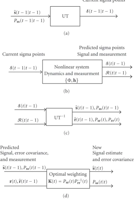
Figure2: UKF: (a) UT, (b) propagation equations, (c) inverse UT, and (d) update equations.
(ii) Update equations:
s(t|t)=s(t|t−1) +K(t)r(t)−hs(t|t−1),
H(t)∇s(t)h
s(t|t−1)
=
⎡ ⎢ ⎢ ⎢ ⎢ ⎢ ⎢ ⎢ ⎢ ⎢ ⎣
s(t|t−1)−m1
s(t|t−1)−m1
−s(t|t−1) s(t|t−1)
T
.. .
s(t|t−1)−mM
s(t|t−1)−mM−
s(t|t−1)
s(t|t−1)
T
⎤ ⎥ ⎥ ⎥ ⎥ ⎥ ⎥ ⎥ ⎥ ⎥ ⎦ ,
P(t|t)=I−K(t)H(t)P(t|t−1).
(19)
(iii) Kalman gain:
K(t)=P(t|t−1)HT(t)H(t)P(t|t−1)HT(t) +R(t)−1 (20)
with the initializations(0| −1) and its respective covariance
P(0| −1).
4. THE UNSCENTED KALMAN FILTER
The EKF is not the only possible procedure for mitigating the nonlinearity in recursive optimal estimation. Julier and
Uhlmann [29] proposed to use the UKF rather than the EKF
for nonlinear recursive estimation problems and showed that an improved performance may be obtained.
Figure 2summarizes the steps involved in the UKF. The method consists of calculating the mean and covariance of a state vector, undergoing a known nonlinear transform by using the unscented transform (UT). For details on the UT,
the reader is referred toAppendix C.
Denote bys(t−1 | t−1) the current source position
estimate and by Pss(t −1 | t−1) its respective
covari-ance. The method is comprised of four stages. In stage (a),
s(t−1 | t−1) is split intoσ-pointsS(t−1 | t−1)
ap-proximating the probability density function of the state
vec-tor (see [29]). By using this method, the mean and
covari-ance propagate through the nonlinearities better than in the EKF method. However, no claims of optimality hold. Then,
in stage (b), each of theσ-points is undergoing the known
nonlinearity yielding theσ-points of thepredictedstate
vec-tor,S(t | t−1). Theσ-points of the predicted noisy
mea-surement,R(t|t−1), are calculated as well. In step (c), the
σ-points are collected together yielding the predicted values
s(t | t−1) andr(t | t−1). This concludes the
propaga-tion stage of the UKF. In step (d), similar to the convenpropaga-tional
filter, the Kalman gain is calculated byK(t)=Psr(t)P−1
rr(t). Note that the covariance matrices estimates are obtained by the UT. Finally, the update stage is implemented by properly weighting the predicted values and the current measurement
yielding the new source location estimates(t|t) and its
re-spective covariancePss(t|t).
Similar to the EKF, (16) and (2) constitute the state and
measurement equations for the UKF. As the nonlinearity is known, the UKF can be applied for solving the localization problem.
5. THE CRAM ´ER-RAO LOWER BOUND
Calculating a bound for the performance of the localizer in the dynamic case is a cumbersome task. To get a rough
es-timate of the predicted performance, following [14], we
as-sume a simplified model of the source locations. Specifically,
we assume that the true range difference readings in the
mea-surement equation (2) are contaminated by Gaussian
dis-tributed noise with zero-mean and covariance matrix Cv.
Note that the existence of directional interferences and rever-beration phenomenon might cause high level of noise cor-relation between microphone pairs and across time. More-over, in high noise level the TDOA estimation algorithm might produce readings related to the directional noise source, causing multimodal noise distribution. Nevertheless,
for simplicity, we start by assuming (like Huang et al. [14])
Huang et al. [14] calculated the CRLB in Cartesian coor-dinates:
Js(t)=GTC−1
v G, (21)
where
G=
⎡ ⎢ ⎢ ⎢ ⎢ ⎢ ⎢ ⎢ ⎢ ⎢ ⎣
s(t)−m1
s(t)−m1−s(t)
s(t)
T
.. .
s(t)−mM
s(t)−mM−s(t)
s(t)
T
⎤ ⎥ ⎥ ⎥ ⎥ ⎥ ⎥ ⎥ ⎥ ⎥ ⎦
. (22)
Note that as no temporal information was used, the obtained result is time independent. When temporal information is used, the calculations become too complex to be evaluated
analytically. However, we may assume that the obtainable bound should be lower.
It is interesting to evaluate the CRLB in polar coordi-nates. Define the transformation from the Cartesian
coor-dinatess(t)=[xs(t) ys(t) zs(t)]T to the polar coordinates
sp(t)[φs(t) θs(t) ρs(t)]Tas
ρs(t)=x2
s(t) +ys2(t) +z2s(t),
φs(t)=cos−1
⎛ ⎜
⎝ xs(t)
x2
s(t) +ys2(t)
⎞ ⎟ ⎠,
θs(t)=sin−1
zs(t) ρs(t)
.
(23)
The Jacobian of the transformation (in Cartesian coordinates terms) can be easily verified to be
Ps(t)=
⎡ ⎢ ⎢ ⎢ ⎢ ⎢ ⎢ ⎢ ⎢ ⎢ ⎢ ⎢ ⎢ ⎣
− ys(t)
x2
s(t) +ys2(t)
xs(t) x2
s(t) +ys2(t) 0
− zs(t)xs(t)
x2
s(t) +ys2(t) +z2s(t)
x2
s(t) +y2s(t)
− zs(t)ys(t)
x2
s(t) +y2s(t) +z2s(t)
x2
s(t) +ys2(t)
x2
s(t) +y2s(t) x2
s(t) +ys2(t) +z2s(t) xs(t)
x2
s(t) +y2s(t) +z2s(t)
ys(t)
x2
s(t) +ys2(t) +zs2(t)
zs(t)
x2
s(t) +y2s(t) +z2s(t)
⎤ ⎥ ⎥ ⎥ ⎥ ⎥ ⎥ ⎥ ⎥ ⎥ ⎥ ⎥ ⎥ ⎦ .
(24)
Therefore, the CRLB in polar coordinates is given by
Jsp(t)=Ps(t)Js(t)Ps(t)T. (25)
In a typical TDOA-based localization scenarios, the mi-crophone array has small interelement spread relative to the source position. As the microphone separation distance
is relatively small, it allows for an efficient calculation of
the TDOA readings. In such circumstances, as we will also
demonstrate by our simulative study of Section 6, the
ob-tainable performance in polar coordinates (concerning only the estimate of the azimuth and the elevation angles in far-field scenario) is superior to the obtainable performance in Cartesian coordinates. For that reason we will present throughout this work the results transformed into polar co-ordinates.
6. EXPERIMENTAL STUDY
In this section we compare the performance obtained by the various localization methods presented in this work. We start
by evaluating the CRLB for a simplified unimodal scenario. This calculation leads us to a conclusion that the mean-ingful information lies in the azimuth and elevation angles rather than in the Cartesian coordinates or the range
infor-mation. Fortunately, these angle estimates are sufficient for
camera steering applications. We proceed by assessing the performance of five localization methods presented in this work. Namely, the two nontemporal methods (LCLS and Gauss iterations) and the three spatial-temporal methods (RG, EKF, and UKF). The methods are first assessed by using artificially contaminated true TDOA readings, in which the speaker is moving along a helix-shaped trajectory. We then proceed with a more realistic scenario for which the available data are estimated TDOA readings obtained from alternating speakers. The TDOA readings are extracted by a previously
proposed method, which exploits speech nonstationarity [8].
It was shown that this method (notated RS1 in [8])
outper-forms other state-of-the-art algorithms.
6.1. Test scenario
A set of eight microphones is placed on a sphere of radius
−2 0
2 4
6 −2 0
2 4
6
−2
−1 0 1 2
x(m) y(m)
z
(m)
Source Mic Noise
Trajectory (3D)
Figure3: Speaker trajectory, noise position, and microphones po-sitions.
mT0 =[0 0 0], at the following positions:3
mT1 =
0.9 0 0, mT2 =
0.45 0.7794 0,
mT3 =
−0.45 0.7794 0, mT4 =
−0.9 0 0,
mT5=−0.45 −0.7794 0, mT6=0.45 −0.7794 0,
mT7 =0 0 0.9, mT8 =0 0 −0.9.
(26)
The speaker trajectory is set to a helix with a radius ofR =
1.5 m, given in Cartesian coordinates by (27) and shown in
Figure 3:
xs(t)=R
cos
t
R
+ 2.5
,
ys(t)=R
sin
t
R
+ 2.5
,
zs(t)= 10t −1.5.
(27)
The main axis of the helix is parallel to the z-axis, 3.75 m
away from the origin. The speaker completes one full circle,
2πRmeters long, in 2πRseconds, hence its tangent speed is
1 m/s. The speaker speed along thez-axis is set to 1/10 m/s.
The time span of the trajectory ist ∈ [0,T] and the total
duration of the movement isT=30 s. The entire scenario is
depicted inFigure 3.
3All dimensions are in meters.
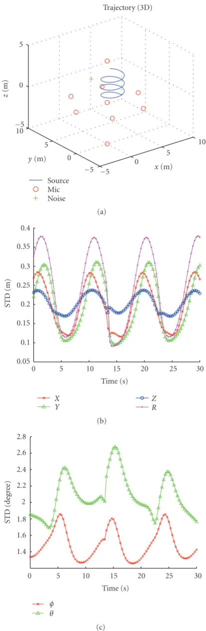
6.2. The CRLB evaluation
We now calculate the CRLB for the tested scenario. We
as-sume that the true range difference (or, equivalently, the
TDOA) readings are contaminated by a unimodal Gaussian distributed noise signal, with zero mean and standard
devi-ation (STD) ofσv = 0.2 m in each coordinate. This STD is
equivalent to 4.7 samples at a sample rate ofFs =8000 Hz.
Under these conditions, the CRLB is calculated for both Cartesian and polar coordinates using the derivations in
Section 5. The resulting bound (in meters for the Cartesian coordinates and the range, and in degrees for the azimuth
and elevation angles) is depicted inFigure 4. The CRLB
nat-urally depends on the source position. Using (27), we give
the CRLB as a function of the time instant, as it completely parameterizes the speaker’s trajectory. Note that the Carte-sian coordinates, as well as the range, cannot be accurately estimated in this scenario. Actually, the obtainable STD ren-ders the estimated quantity useless. However, the azimuth and elevation angles may be estimated in high accuracy. For-tunately, for camera steering applications, estimation of the
azimuth and elevation angles suffices. Note also that the
pre-sented CRLB serves as a bound to the nontemporal methods alone, since past measurements are disregarded at each time instant.
Finally, we comment that the CRLB can be dramati-cally reduced to an acceptable level (especially, for the Carte-sian coordinates and range) if, for instance, we set the
ra-dius of the array to 5 m instead of 0.9 m. The new
micro-phone constellation and the associated CRLB is shown in
Figure 5. However, the larger dimensions of the array impose huge computational burden on the first stage of the localizer, namely, the TDOA extraction. In this work, we will concen-trate on the more practical scenario, where the speaker dis-tance from the microphones is significantly larger than the array dimensions.
6.3. Artificially contaminated range difference
The setup presented inSection 6.1is evaluated by five
local-ization methods. The true range differences are assumed to
be contaminated by spatially and temporally white Gaussian
noise with covariance matrix Cov{v(t)} =σ2
vI,σv=0.2 m.
The first localization algorithm is the LCLS method,
pre-sented by Huang et al. [14]. The second is the batch Gauss
method (denoted BG) with three iterations at each time
in-stant. The third is the RG with forgetting factorα = 0.85.
We emphasize that no attempt to optimize this quantity was
made. The value ofα = 0.85 was set as a compromise
be-tween fast adaptation requirements and stable estimation. The fourth is the EKF method evaluated with random-walk
model having driving noise with a STD of 0.5 m along each
Cartesian coordinate, that is,Q(t)= 0.52I
3. This value was
0 5 10 15 20 25 30 0
2 4 6 8 10 12
Time (s)
STD
(m)
X
Y ZR
(a)
0 5 10 15 20 25 30
7 7.5 8 8.5 9 9.5
Time (s)
STD
(deg
ree)
φ θ
(b)
Figure4: CRLB results for position estimate along the speaker trajectory for the scenario inFigure 3with array radius set to 0.9 m. (a) Cartesian coordinates and range. (b) Azimuth (φ) and elevation (θ) angles.
overestimated to R(t) = 10σ2
vI; σv = 0.2 m. To allow a
slight decay of past estimates, we set the transition matrix
to the valueΦ=0.99I. The fifth tested method is the UKF
method using the same setup as the EKF. No attempt was made to adapt the parameters of the filters to a given sce-nario. One thousand Monte Carlo trials are performed to obtain a meaningful evaluation of the root mean square er-ror (RMSE) of the angles estimate. The results for this setup
are depicted inFigure 6.
We have also repeated this experiment with an additional
point noise source which is placed at the [0.5 4 1.5]T
co-ordinate (seeFigure 3). By replacing 20% of the range
dif-ference readings by readings associated with the point noise location rather than the speech source position, we aim to simulate a scenario where, due to the directional interferer, the first localization stage, that is, the estimation of TDOA
values, is disrupted by the point noise source.4 Results for
this scenario are depicted inFigure 7. As can be seen, for both
scenarios, the LCLS method has better performance than the Gauss iterations method. However the RG which exploits the temporal information obtains better results. The EKF and the UKF methods remarkably outperform the other meth-ods, with slight advantage to the latter. Overall, the results of the Kalman filter-based methods demonstrate acceptable performance even in these harsh conditions. By comparing
Figures6and7, we see that the obtainable performance in
the first, anomaly-free case is better than that of the latter scenario. We also remark, that no advantage was gained by directly estimating the polar coordinates rather than
trans-4We note that the 80% true range difference readings are still corrupted by
the white Gaussian noise, as in the previous scenario.
forming the estimates of Cartesian coordinates into polar co-ordinates.
We conclude this section by presenting inFigure 8a
typ-ical realization for the tracking ability of both the EKF and UKF methods for the directional interference case. The small bias depicted in the figure is probably due to the fact that the Kalman-based localizers cannot track the fast maneuvering speaker in this specific setup.
6.4. Switching scenario
We proceed by testing a more realistic scenario. Consider the following simulation which is typical to a video conference
scenario. Two speakers located at two different and fixed
lo-cations alternately speak. The camera should be able to ma-neuver from one person to the other. For this scenario, simu-lation is conducted with one speaker located at the polar
po-sition [φ=(π/4) rad θ=(π/4) rad R=1.5 m] and the other
at [φ=(3π/4) rad θ=(π/3) rad R=1.5 m]. A directional
interference is placed at the position [φ = (π/2) rad θ =
(π/4) rad R=1.0 m]. Six microphones were mounted at the
following positions (in meters), relative to the reference mi-crophone (which is at the axes origin):
mT1 =0.3 0 0, mT2 =−0.3 0 0,
mT3 =0 0.3 0, mT4 =0 −0.3 0,
mT5 =0 0 0.3, mT6 =0 0 −0.3.
(28)
10 5
0
−5
10 5
0
−5
−5 0 5
y(m)
x(m)
z
(m)
Source Mic Noise
Trajectory (3D)
(a)
0 5 10 15 20 25 30
0.05 0.1 0.15 0.2 0.25 0.3 0.35 0.4
Time (s)
STD
(m)
X
Y ZR
(b)
0 5 10 15 20 25 30
1.4 1.6 1.8 2 2.2 2.4 2.6 2.8
Time (s)
STD
(deg
ree)
φ θ
(c)
Figure5: CRLB results. (a) Test scenario with array radius set to 5 m. (b) Cartesian coordinates and range. (c) Azimuth (φ) and ele-vation (θ) angles.
the true range differences, estimated TDOA values
(equiva-lently, range differences) were used. We note that any method
for TDOA extraction can be used in conjunction with our lo-calization algorithm. However, to give specific simulations, we used TDOA readings, extracted from the noisy
micro-phone data, by the RS1 algorithm described in [7,8]. For
that estimation stage, room reverberation (set to
reverbera-tion time ofTr =0.25 s) and the directional interferer were
taken into account. Room reverberation was simulated by the image method[30]. Mean SNR level was set to 10 dB. The same setup for the localization methods is applied here as well. Namely, the EKF and UKF localizers still use the ran-dom walk model though a better choice might have been as-serted.
Figure 9presents the azimuth angle estimates obtained
by the five methods. Figure 10 presents the respective
ele-vation angle estimates. As can be seen from the plots, the temporal methods, especially the EKF and UKF algorithms, clearly outperform the other methods. The transition in-stances are the main cause of errors in this scenario. While the batch methods (Gauss and LCLS) demonstrate unsta-ble behavior in these regions, the recursive methods demon-strate smooth transition curves due to their inherent mem-ory. Although the Kalman-based methods are not using a valid state-space model, their performance is obviously bet-ter than the nonrecursive methods. The UKF method obtains slightly better results than the EKF method in wide range of parameters’ value selection. The computational burden of both methods is comparable.
7. CONCLUSIONS
We presented both nontemporal and temporal algorithms for talker localization and tracking. The nontemporal meth-ods are commonly used in speech localization applica-tions. Among the two batch methods, the LCLS method outperforms the Gauss method. Three temporal methods were derived. One is within a non-Bayesian framework (RG algorithm) and the other two are within the Bayesian framework, namely, the EKF and UKF algorithms. Both these Kalman filter-based methods are known to be computa-tionally simpler than the particle filter. The UKF method marginally outperforms the EKF method for a wide range of parameters’ values. Nevertheless, the imposed computa-tional burden is almost equivalent. Evaluation of the CRLB showed that for a microphone array with a small interele-ment spread relative to the source position, angle estimates might be obtained reliably (as opposed to the Cartesian co-ordinates estimates). This justifies the use of polar coordi-nates rather than Cartesian coordicoordi-nates in our simulations.
Empirical results demonstrate the effectiveness of using the
0 5 10 15 20 25 30 0
5 10 15 20 25 30 35 40
Time (s)
RMSE
azim
u
th
ang
le
(deg
ree)
BG LCLS RG
EKF UKF (a)
0 5 10 15 20 25 30
0 5 10 15 20 25
Time (s)
RMSE
ele
vation
ang
le
(deg
ree)
BG LCLS RG
EKF UKF (b)
Figure6: RMSE results averaging 1000 trials with white Gaussian noise. (a) Azimuth angle (φ). (b) Elevation angle (θ).
extensions of the Kalman filter, might be able to improve the tracking ability of the algorithms, in particular, at the abrupt changes instances.
APPENDICES
A. GAUSS METHOD
Consider the weighted nonlinear LS problem:
min s(t)
b(t)−fs(t)TWb(t)−fs(t), (A.1)
whereWis an arbitrary weighting matrix. Expandingf(s(t))
to a Taylor series arounds∗(t) and taking only first-order
ap-proximation, we obtain
fs(t)fs∗(t)+∇s(t)f
s∗(t)s(t)−s∗(t). (A.2)
Define the error term(t)b(t)−f(s(t)). Then
(t)b(t)−fs∗(t)− ∇s(t)f
s∗(t)s(t)−s∗(t)
=b(t)−fs∗(t)− ∇s(t)f
s∗(t)s(t)
+∇s(t)f
s∗(t)s∗(t)
=b(t)− ∇s(t)f
s∗(t)s(t),
(A.3)
whereb(t)=b(t)−f(s∗(t)) +∇s(t)f(s∗(t))s∗(t). Using the
gradient matrix definition,F(s∗(t))= ∇s(t)f(s∗(t)), we
ob-tain a linearized LS problem:
min s(t)
b(t)−Fs∗(t)s(t)TWb(t)−Fs∗(t)s(t).
(A.4)
The LS solution is given by
s(t)=FTs∗(t)WFs∗(t)−1
FTs∗(t)
×Wb(t)−fs∗(t)+Fs∗(t)s∗(t)
=s∗(t) +FTs∗(t)WFs∗(t)−1FTs∗(t)
×Wb(t)−fs∗(t).
(A.5)
Since this solution is valid for anys∗(t), we can use it
itera-tively to obtain the Gauss method:
s(l+1)(t)=s(l)(t) +FTs(l)(t)WFs(l)(t)−1
×FTs(l)(t)Wb(t)−fs(l)(t) (A.6)
starting from an initial guesss(0)(t).
B. RLS FOR MULTIPLE READINGS
Assume a scenario in which for each time instant we haveK
0 5 10 15 20 25 30 0
5 10 15 20 25 30 35 40 45 50
Time (s)
RMSE
azim
u
th
ang
le
(deg
ree)
BG LCLS RG
EKF UKF (a)
0 5 10 15 20 25 30
0 5 10 15 20 25
Time (s)
RMSE
ele
vation
ang
le
(deg
ree)
BG LCLS RG
EKF UKF (b)
Figure7: RMSE results averaging 1000 trial with white Gaussian noise and 20% anomaly. (a) Azimuth angle (φ). (b) Elevation angle (θ).
0 5 10 15 20 25 30
0 10 20 30 40 50 60 70
Time (s)
A
zim
uth
ang
le
(deg
re
e)
True EKF UKF
(a)
0 5 10 15 20 25 30
−15
−10
−5 0 5 10 15 20 25
Time (s)
Ele
vation
ang
le
(deg
re
e)
True EKF UKF
(b)
Figure8: One realization of tracking results with white Gaussian noise and 20% anomaly for EKF and UKF. (a) Azimuth angle (φ). (b) Elevation angle (θ).
parameter vectorθ ∈Rp by a linearK×ptransformation
H(τ):
z(τ)≈H(τ)θ. (B.1)
The approximation is due to the fact that the measurements
are noisy or due to slight modelling errors.τ = 1, 2,. . .,t
time instants can be augmented to a matrix formz(1 :t)≈
H(1 :t)θwhere
z(1 :t) ⎡ ⎢ ⎢ ⎢ ⎢ ⎢ ⎣
z(1) z(2) .. . z(t)
⎤ ⎥ ⎥ ⎥ ⎥ ⎥
⎦, H(1 :t)
⎡ ⎢ ⎢ ⎢ ⎢ ⎢ ⎣
H(1) H(2)
.. . H(t)
⎤ ⎥ ⎥ ⎥ ⎥ ⎥
0 5 10 15 20 25 30
−200
−150
−100
−50 0 50 100 150 200 250 300
Time (s)
φ
(deg
re
e)
True Estimated
LCLS method
(a)
0 5 10 15 20 25 30
−200
−150
−100
−50 0 50 100 150 200 250 300
Time (s)
φ
(deg
re
e)
True Estimated
Gauss method
(b)
0 5 10 15 20 25 30
−200
−150
−100
−50 0 50 100 150 200 250 300
Time (s)
φ
(deg
re
e)
True Estimated
RG method
(c)
0 5 10 15 20 25 30
−200
−150
−100
−50 0 50 100 150 200 250 300
Time (s)
φ
(deg
re
e)
True Estimated
EKF method
(d)
0 5 10 15 20 25 30
−200
−150
−100
−50 0 50 100 150 200 250 300
Time (s)
φ
(deg
re
e)
True Estimated
UKF method
(e)
0 5 10 15 20 25 30
−80
−60
−40
−20 0 20 40 60 80
Time (s)
θ
(deg
re
e)
True Estimated
LCLS method
(a)
0 5 10 15 20 25 30
−80
−60
−40
−20 0 20 40 60 80
Time (s)
θ
(deg
re
e)
True Estimated
Gauss method
(b)
0 5 10 15 20 25 30
−80
−60
−40
−20 0 20 40 60 80
Time (s)
θ
(deg
re
e)
True Estimated
RG method
(c)
0 5 10 15 20 25 30
−80
−60
−40
−20 0 20 40 60 80
Time (s)
θ
(deg
re
e)
True Estimated
EKF method
(d)
0 5 10 15 20 25 30
−80
−60
−40
−20 0 20 40 60 80
Time (s)
θ
(deg
re
e)
True Estimated
UKF method
(e)
The WLS solution for θ using nonnegative weight matrix
W(1 :t) (of sizeKt×Kt) is given by
θ=H(1 :t)TW(1 :t)H(1 :t)−1H(1 :t)TW(1 :t)z(1 :t). (B.3)
Our goal is to evaluate (B.3) recursively. If the parameters
slowly change, a common approach is to apply a diagonal
weight matrix W(1 :t) with powers of a forgetting factor
0 < α ≤ 1 along its diagonal. Note that for measurements associated with the same time instant, we wish to apply the same factor, since equations of the same time instant have equal importance. Such weight matrix can be represented re-cursively as
W(1 :t)= αW(1 :OTt−1) OI
!
, W1:1=I, (B.4)
whereI andO stand for the identity and zero matrices of
sizesK×K and (t−1)K×K, respectively. At first glance it
seems that a recursive solution to (B.3) necessitates (K×K
)-matrix inversion in each RLS iteration. However, in practice, the complexity can be further reduced. This is obtained by applying the well-known RLS algorithm with a minor twist. Consider a single equation. If this equation belongs to one of
theK equations constituting the current time instant (but
not the first one), a forgetting factor of 1 should be used.
However, if this equation is the first at the new time instantτ,
a forgetting factorα≤1 must be used instead. Thus, in order
to derive a recursion, where the update stage considers only asingleequation, the forgetting factor should vary. Notating
the time instant byτ(τ =1, 2,. . .) and the sequential
num-ber of the equation by (τ−1)K+k(wherek∈ {1,. . .,K}),
the forgetting factor becomes
forgetting factor=
⎧ ⎨
⎩α
, k=1,
1, otherwise. (B.5)
It is easily verified that a matrix inversion is not necessary in this case.
C. THE UNSCENTED TRANSFORM
Letxbe anL-dimensional random vector with mean ¯xand
covariance matrixPxx. Lety= f(x) be a nonlinear
transfor-mation from the random vectorxto another random vector
y. The first- and second-order statistics of the vectoryshould
be calculated. We briefly summarize the method proposed in
[29]. The mean and covariance ofxcan be presented by the
2L+ 1σ-points
X0=x¯,
Xl=x¯+
(L+λ)Pxx
l, l=1,. . .,L,
Xl+L=x¯−
(L+λ)Pxx
l, l=1,. . .,L,
(C.1)
where (%(L+λ)Pxx)lis thelth row or column of the
corre-sponding matrix square root andλ =α2(L+κ)−L.α
de-termines the spread of the sigma points. α = 1 was used
throughout our simulations.κis a secondary scaling
parame-ter. The choiceκ=3−Lmaintains the kurtosis of a Gaussian
vector. Throughout our simulations,κis set to 0.
Define the weights
W(m)
0 =λ/(L+λ),
W(c)
0 =λ/(L+λ) +
1−α2+β,
W(m)
l =Wl(c)=1/2(L+λ), l=1, 2,. . ., 2L,
(C.2)
whereβis used to incorporate prior knowledge of the
distri-bution (β=2 for Gaussian distributions). A proper choice of
these parameters and its influence on the obtainable perfor-mance is still an open topic. Then the mean and covariance of
the vectorycan be calculated using the following procedure.
(1) Constructxσ-points:Xl,l=0,. . ., 2L.
(2) Transform each point to the respective y σ-points:
Yl=f(Xl),l=0,. . ., 2L.
(3) Use weighted averaging ¯y ≈&2L
l=0Wl(m)Ylto estimate
ymean.
(4) Use weighted outer productPyy≈&2L
l=0W (c)
l (Yl−y¯)(Yl−
¯
y)Tto estimateycovariance andPxy≈&2L
l=0W (c)
l (Xl−
¯
x)(Yl−y¯)Tto estimate the cross-covariance betweenx
andy.
The benefits of using the UT are presented in [29,31].
REFERENCES
[1] C. H. Knapp and G. C. Carter, “The generalized correlation method for estimation of time delay,”IEEE Transactions on Acoustics, Speech, and Signal Processing, vol. 24, no. 4, pp. 320– 327, 1976.
[2] M. Brandstein and H. Silverman, “A robust method for speech signal time-delay estimation in reverberant rooms,” in Pro-ceedings of the IEEE International Conference on Acoustics, Speech, and Signal Processing (ICASSP ’97), vol. 1, pp. 375–378, Munich, Germany, April 1997.
[3] A. St´ephenne and B. Champagne, “A new cepstral prefiltering technique for estimating time delay under reverberant condi-tions,”Signal Processing, vol. 59, no. 3, pp. 253–266, 1997. [4] J. Benesty, “Adaptive eigenvalue decomposition algorithm for
passive acoustic source localization,”The Journal of the Acous-tical Society of America, vol. 107, no. 1, pp. 384–391, 2000. [5] S. Doclo and M. Moonen, “Robust adaptive time delay
estima-tion for speaker localizaestima-tion in noisy and reverberant acoustic environments,”EURASIP Journal on Applied Signal Processing, vol. 2003, no. 11, pp. 1110–1124, 2003.
[6] T. Dvorkind and S. Gannot, “Speaker localization in a rever-berant environment,” inProceedings of the 22nd IEEE Conven-tion of Electrical and Electronics Engineers in Israel (IEEEI ’02), pp. 7–9, Tel-Aviv, Israel, December 2002.