R E S E A R C H
Open Access
Robust surface registration using
N
-points
approximate congruent sets
Jian Yao
*, Mauro R Ruggeri, Pierluigi Taddei and Vítor Sequeira
Abstract
Scans acquired by 3D sensors are typically represented in a local coordinate system. When multiple scans, taken from different locations, represent the same scene these must be registered to a common reference frame. We propose a fast and robust registration approach to automatically align two scans by finding two sets ofN-points, that are approximately congruent under rigid transformation and leading to a good estimate of the transformation between their corresponding point clouds. Given two scans, our algorithm randomly searches for the best sets of congruent groups of points using a RANSAC-based approach. To successfully and reliably align two scans when there is only a small overlap, we improve the basic RANSAC random selection step by employing a weight function that approximates the probability of each pair of points in one scan to match one pair in the other. The search time to find pairs of congruent sets ofN-points is greatly reduced by employing a fast search codebook based on both binary and multi-dimensional lookup tables. Moreover, we introduce a novel indicator of the overlapping region quality which is used to verify the estimated rigid transformation and to improve the alignment robustness. Our framework is general enough to incorporate and efficiently combine different point descriptors derived from geometric and texture-based feature points or scene geometrical characteristics. We also present a method to improve the matching effectiveness of texture feature descriptors by extracting them from an atlas of rectified images recovered from the scan reflectance image. Our algorithm is robust with respect to different sampling densities and also resilient to noise and outliers. We demonstrate its robustness and efficiency on several challenging scan datasets with varying degree of noise, outliers, extent of overlap, acquired from indoor and outdoor scenarios.
1 Introduction
In the past decade, there was a growing interest in 3-D reconstruction and realistic 3-D modelling of large-scale scenes such as urban structures. Applications of such models include virtual reality, cultural heritage, urban planning, and architecture. Commonly, these applica-tions require a combination of laser sensing technology with traditional digital photography.
Applications that employ only digital images extract 3-D information using either a single moving camera or a multi camera system, such as a stereo rig. In both cases, the system extracts and matches distinctive features (typically points) among the available images and esti-mates both their 3-D positions and the camera para-meters [1,2]. It is then possible to exploit the result of this first step to perform a dense point reconstruction
by estimating a depth map for each image [3,4]. On one hand, these approaches are useful for those applications requiring a robust and low-cost acquisition system. On the other hand, laser sensing technology yields much higher precision and resolution. Thus, the laser sensing technology represents an effective and powerful tool for achieving accurate geometric representations of complex surfaces of real scenes.
In recent years, 3-D laser scanners able to provide satisfying measurement accuracy for different applica-tions become commercially available. These sensors are used to acquire a complex real scene through multiple scans taken from different positions to fully describe the scene while reducing the number of occluded surfaces. For this reason, it is important to employ a systematic and automatic way to align, or register, multiple 3-D scans to represent and visualize them in a common coordinate system. Geometrically, given a point cloudQ considered as reference and a second point cloudP, the * Correspondence: [email protected]
Institute for Transuranium Elements, European Commission-Joint Research Centre (JRC), Ispra, VA, Italy
problem of registration consists in finding the rigid transformationT, which optimally alignsP toQin its coordinate system.
1.1 Related works
The iterative closest point (ICP) algorithm [5] is the de facto standard to compute the rigid transformationT between two point clouds. It is basically an optimization method that starts from an initial estimate ofT and iteratively refines it by generating pairs of corresponding points on the scans and minimizing an error metric, e. g., the sum of squared distances between corresponding points. Although several variants of ICP were presented [6] to improve its efficiency, the main problem is to achieve a good initial estimate ofT since the ICP opti-mization can easily stop in local minima.
The problem of automatically registering two scans was achieved with a wide variety of methods [7]. Most of these extract sets of feature points, which are auto-matically matched to recover a good approximation of T. Aiger et al. [8] proposed to automatically match congruent sets of four roughly coplanar points to solve the largest common point (LCP) set problem. Congru-ent sets of points have similar shapes defined in terms of point distances and normal deviations. The best match between congruent sets is randomly found by following the RANdom SAmple Consensus (RANSAC) approach [9]. Other approaches use shape descriptors to identify sets of candidate feature points to be matched. Gendalf et al. [10] use a 3-D integral invar-iant shape descriptor to detect feature points, which are matched in sets of three items using a branch-and-bound algorithm. Other interesting shape descriptors invariant with respect to rigid transformation are used to identify feature points, such as scale invariant fea-ture transforms (SIFT)s [11,12] or Harris corners [12] extracted from reflectance images, 3-D SIFT-like descriptors extracted from triangle meshes approximat-ing the point clouds [13], wavelet features [14], inten-sity-based range features [15], spin images [16,17], and extended Gaussian images [18].
Methods to automatically recover the rigid transfor-mations from matching sets of higher-level features were also presented. The advantage of these approaches is the reduction of the search space identified by two small sets of features, which results in efficient match-ing, but that should account for extra computation time due to scene segmentation or feature detection. Among the feature types presented the most interesting are: lines [19,20], planes [19-22], circles [23], spheres [24] and other fitted geometric primitives [25].
Other studies proposed to formulate the registration as an energy optimization problem that does not need any explicit set of point correspondences. Silva et al.
[26] proposed to use an enhanced genetic algorithm to solve the range image registration problem using a robust surface interpenetration measure. Boughorbel et al. [27] defined an energy minimization function based on Gaussian fields to solve the 3-D automatic registration.
The last relevant class of registration approaches is based on modelling the alignment of two point sets as an assignment problem, where the probability of a point in one set to has a correspondence in the other set is estimated and maximized with expectation maximiza-tion (EM) algorithms. Popular methods following this approach are known as SoftAssign [28] and EM-ICP [29], which are both based on entropy maximization principles, but imposing different constraints for pro-blem optimization, i.e., a two-way constraint embedded into the deterministic annealing scheme for SoftAssign and a one-way constraint for the EM-ICP. A detailed review and analysis of these methods was provided in [30], where Liu proposed a method to overcome SoftAs-sign and EM-ICP limitations based on modelling the registration problem as Markov chain of thermodynamic systems and on an entropy model derived from the Lya-punov function. Furthermore, fast implementations on GPU of the SoftAssign and EM-ICP algorithms were recently presented by Tamaki et al. [31].
1.2 Our algorithm
Our method utilizes 3-D points (possibly associated with point descriptors, as it is described in Section 6) to achieve automated registration. It automatically aligns two scans by finding twoN-points approximate congru-ent sets leading to a good estimate of the transformation T between the corresponding point clouds.T is then further refined via the ICP algorithm.
Given two scans P andQ, our algorithm randomly searches for sets of congruent groups of points inPand Q. Corresponding groups are then used to estimate a rigid transformationT to align P toQ. The optimal transformation is recovered following a RANSAC opti-mization [9], which iterates the following steps until a good solution to the problem is found or the number of iterations exceeds a predefined thresholdImax:
1)Random selection of aN-points baseBpinP.
2)Approximate congruent group selectionofN
-points bases inQ. The definition of approximate point set congruence is described in Section 2. This selection is achieved by using a general codebook to efficiently find approximate congruent points bases under rigid transform by exploiting combinations of feature point descriptors when available (see Section 3).
3) Estimation of the transformationT between P
P and each extracted approximate congruent N -points baseBpinQ.
4) Verificationof the transformation.T is verified
using all possibly corresponding points after the alignment. The verification employs our proposed quality-based largest common pointset (QLCP) mea-sure described in Section 4.4.
The best transformation is selected as the one yielding the best QLCP measure and then further refined with the ICP algorithm. As in [20], we present a variant of this RANSAC-based algorithm, which improves the random selection step by employing a weight function approximat-ing the probability of each pair of features inP to be matched with one inQ. We call this variant as probability-based RANSAC approachand describe it in Section 4.1.
Our algorithm is robust with respect to different sam-pling densities and the typical noise introduced by laser scanner acquisition. This is achieved by employing suita-ble point sampling approaches described in Section 5, and by using feature points and their descriptors to effec-tively constrain rigid transformations on noisy point sets.
Through our proposed matching framework presented in Sections 2 and 3, we efficiently match points and point pairs in a multi-dimensional space defined by a set of available geometric and texture feature descriptors and geometrical constrains of a set of sampled points. The matching is performed by combining suitable metric functions to compare the provided descriptors.
Any type of features carrying suitable distance func-tions to be compared can be easily integrated into our matching framework. The major benefit of this approach is to make possible efficient customizations for specific applications aiming at relevantly improving the registra-tion performance in terms of robustness, accuracy, and execution time.
We also present a method to improve the matching effectiveness of texture features extracted from typical spherical reflectance images acquired by laser scanners. It consists in extracting features from atlases of rectified perspective images constructed by sampling the reflec-tance image spherical field of view at suitable angles. This approach mitigates the effect of spherical distortion on the resulting feature signatures so that they can be matched with higher reliability.
The robustness, accuracy and efficiency of our method were overall evaluated on several challenging scan data-sets acquired from indoor and outdoor scenes as described in Section 7.
2 Approximate point set congruence
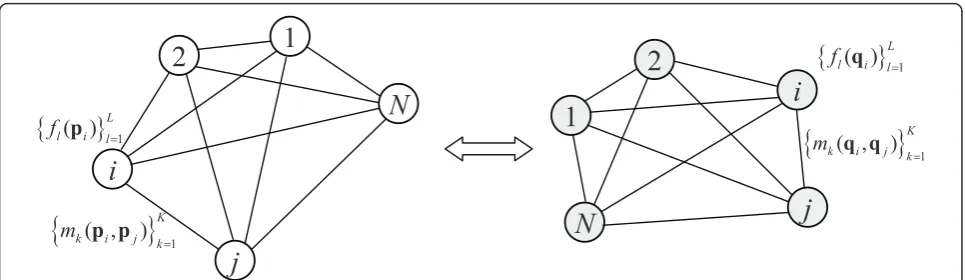
Given two point sets P and Q, we assume Bp={pi|pi∈P}Ni=1andBq={qi|qi∈Q}Ni=1to be the two
corresponding N-points bases fromP andQ, respec-tively. This means that for each point pi∈Bp there
exists one and only one corresponding pointqi∈Bq.
We consider the two sets to be congruent, if they are approximatively similar in shape and have a similar dis-tribution in 3-D space. We define both a similarity score function and a binary similarity score function in order to measure the congruency of two matching N-points bases as follows.
Given a pointpi∈Bp, we characterize it using a set of
Llocal descriptors, i.e.,{fl(pi)}Ll=1. Similarly, for each pair of points (pi, pj) inBp, we define a set of K
measure-ments{mk(pi,pj)}Kk=1. TheLdescriptors and theK mea-surements characterize a N-points base in terms of point features and point pairs relations (see Figure 1). These values are then used to define the congruency of the two differentN-points basesBpandBq.
For each type of local descriptor or points pair mea-surement, we define a similarity differencefunctiond(·, ·) that is invariant under rigid transformation of each singleN-points base. In particular, given two descriptors or measurementsvpand vq, thend(vp,vq) is represented
by a real positive value that states how different the two descriptors or measurements are.
We also define a set ofboolean similarity measures
s(vp,vq) =b(d(vp,vq),t), (1)
wheretis a threshold value associated to the particu-lar feature descriptor or measurement and b(·, ·) is a boolean function defined as:
b(x,t) =
1 x≤t,
0 x>t. (2)
The set of functions {d(·, ·)} are then composed together to define asimilarity score sc(Bp,Bq)between two congruentN-points bases as follows:
sc(Bp,Bq) =sfc(Bp,Bq) +sm
c(Bp,Bq), (3)
where sf
c is the term related to the local descriptors
andsmc is the term related to the similarity measures of points pairs. These two terms are defined as:
sfc(Bp,Bq) = 1
Nf N
i=1 L
l=1
wfl·
⎛
⎝1−min
d(fl(pi),fl(qi)),t f l
tfl
⎞
⎠, (4)
sm c(Bp,Bq) =
1 Nm
i,j= 1· · ·N i=j
K
k=1 wm
k·
1−min(d(mk(pi,pj),mk(qi,qj)),tmk)
tm k
,
(5)
where {wfl} and {wmk} are user-defined weights,
Nm= 2N(N−1)
K
Nm= 2N(N−1)Kk=1wmk are normalization factors.
Notice that sc is defined such that its values fall in the
range [0, 1], where a higher value represents a higher similarity between the twoN-points bases.
Similarly, we define the binary similarity score sc(Bp,Bq)between twoN-points bases as:
s(Bp,Bq) = N
i=1
L
l=1
sl(fl(pi),fl(qi))
· ⎛ ⎜ ⎜ ⎜ ⎜ ⎜ ⎝
i,j= 1· · ·N i=j
K
k=1
sk(mk(pi,pj),mk(qi,qj)) ⎞ ⎟ ⎟ ⎟ ⎟ ⎟ ⎠
. (6)
where sc(Bp,Bq)represents the product of all boolean similarities associated to the matching points of the two sets. We considerBpandBqto be approximate
congru-ent only ifs(Bp,Bq) = 1.
In order to evaluate theN-points base congruence, we need to define which local point descriptors {fl(·)} and
points pair measurements functions {mk(·, ·)} to employ,
their corresponding similarity differences {d(·, ·)} and scalar thresholds {t}. We consider as first points pair measurement the Euclidean distancem1(pi, pj) = ||pi -pj|| and define its similarity difference as:
d1(m1(pi,pj),m1(qi,qj)) = 1−
min(m1(pi,pj),m1(qi,qj)) max(m1(pi,pj),m1(qi,qj))
. (7)
If the surface normal at each point is available, we define the second points pair measurementm2(pi, pj) =
nangle(n(pi),n(pj)), wheren(p) denotes the surface
nor-mal of the point p and nangle(·, ·) denotes the minimal
angle between the two surface normals. Its similarity dif-ference is defined as:
d2(m2(pi,pj),m2(qi,qj)) = |m2(pi,pj)−m2(qi,qj)(8)|.
If the reflectance or colour images associated with the range scans are available we can extract the correspond-ing feature points (e.g., SIFT or SURF feature points [32]) associated with each 3-D point ofBpandBq. The
corresponding local feature descriptors can be used to define a suitable similarity difference.
In some application, it is possible to exploit some information about the environment to define additional descriptors. This is the case of scans representing struc-tural scenes with one common and main normal direc-tion (ground floor scene) or environment with three common orthogonal normal directions (orthogonal scene). For instance, in an indoor/outdoor scene with a common and main ground floor plane, all points lying on the ground plane roughly have the same normal directions. The type of a structural scene can be auto-matically detected and classified by clustering the sur-face normals.
In the case ofground floor scene, we initially transform all points in P andQ to align their corresponding ground floor normals to thez-axis. Then for each point
p = (px, py, pz)⊤, an additional local descriptor can be defined as fz(p) = nangle(p, nz), where nzdenotes the
direction of z-axis, i.e., nz= (0, 0, 1)⊤. fz(p) represents
the inclination of the surface passing through p w.r.t. the ground. Its similarity difference is defined as:
dfz(fz(pi),fz(qi)) = |fz(pi)−fz(qi)|. (9)
In addition, we can introduce another points pair measurementmz(pi,pj) =pzi−pzj, i.e., the height differ-ence between the two points. Its corresponding similar-ity difference can be defined as:
dmz(mz(pi,pj),mz(qi,qj)) = |mz(pi,pj)−mz(qi,qj)|.(10)
If both P andQare acquired from an orthogonal scene, P andQare first transformed to align their cor-responding three orthogonal point normals to thex-,y -andz-axis, respectively. Then, we exploit two more local descriptors defined as fx(p) = nangle(p, nx) and fy(p) =
nangle(p, ny), where nx = (1, 0, 0)⊤ and ny = (0, 1, 0)⊤.
1
i
j
N
1
N
i
j
^
( , )
`
1K
k i j k
m
p p
^
( )
`
1 Ll i l
f
p
^
( , )`
1K
k i j k
m q q
^
( )
`
1 Ll i l
f
q
2
2
These descriptors represent the inclinations of the sur-face passing throughpw.r.t. the additional main axesnx
and ny, respectively. In addition, we introduce two other
points pair measurements mx(pi,pj) =px
i −pxj, and
my(pi,pj) =pyi −pyj. The corresponding similarity differ-ence offx,fy,mx andmyare defined in the same way as
in Equations (9) and (10), respectively.
3 Fast search codebook
Using the criteria defined in the previous section, we are able to evaluate the congruency of two givenN-points bases. To perform the registration, we need to couple aN -points baseBp∈Pwith theN-points baseBq∈Qhaving
a high-similarity score. This task requires a search over all possibly congruentN-points bases inQ. Using exhaustive search approaches is impractical due to the large number of candidates inQ. To solve this problem, we build a code-book fromP andQcomposed of two different data struc-tures used to perform a fast search of possibly corresponding points (as described in Section 3.1) and point pairs (as described in Section 3.2). In particular, we employ a boolean tableSfused to detect candidate point
matches inQof a selected point pi∈P and a multi-dimensional tableSmused to detect candidate point pair
matches of a selected pair of points(pi,pj)∈P. If the number of all detected congruentN-points bases is still large, we further need to compute a similarity score betweenBpand each detected base inQin order to sort
them and then consider only the best ones.
The used codebook is, thus, composed of a booleanm × n table and a floating-pointn × n × K tablea, where m= |P|, n= |Q|and K denote the number of used points pair measurements. The required memory for Sf
increases as O(mn) and for Sm increases as O(n2)
(assumingK≪n).
Our algorithm detects candidate congruentN-points bases incrementally. GivenBp∈P, we start by selecting
two points in Bp and collect all congruent 2-points
bases inBq. We then iteratively add points to the
cur-rent selection and grow the set of candidate bases until we reach a set ofN-points bases.
3.1 Point features lookup table
We build Sfas am × nboolean similarity measure table
according to the used local descriptors, wherem= |P|
andn= |Q|, i.e., the sizes ofP andQ, respectively. Each element inSfis defined as:
Sf(pi,qj) = L
l=1
sl(fl(pi),fl(qj)), (11)
where pi∈P and qj∈Q, i= 1. . .m, and j = 1...n. Thus, given a pointpi∈P, we can recover all possibly
matching points inQconsidering theith row ofSf. The
set of candidate matches inQforpiis represented by:
Mf(pi) ={qj|Sf(pi,qj) = 1}qj∈Q. (12)
Notice that, to buildSf, we only make use of the local
feature descriptors. Its size depends on the number of points of both point clouds. In Section 5, we describe several techniques to sample the input acquisitions in order to reduce their sizes.
3.2 Point pairs lookup table
Given a point pair(pi,pj)∈P, we need to efficiently find candidate matching pairs in Q. Using a blind exhaustive search, this would require a comparison with
n(n−1)
2 point pairs. To reduce the searching time, we build a lookup tableSmforQby uniformly quantising
the K-dimensional space formed by the usedKpoints pair measurements {mk(·, ·)}, i.e., the Euclidean distance,
the surface normal minimal angle, the gap difference(s) in the x-, y- or z-axis for structural scenes, etc. The quantisation is achieved by uniformly dividing their cor-responding value ranges intoB1,B2, ...,BKbins,
respec-tively. The range of the Euclidean distance is
[dqmin,dqmax], where dqmin and d
q
max denote the minimal and maximal distances of point pairs inQ. Surface nor-mal mininor-mal angle falls in the range [0,π]. The gap dif-ferences fall in the ranges [-bx,bx], [-by,by] and [-bz,bz],
respectively, wherebx,byand bzrepresent the lengths in
x,y andz-axis of the minimal bounding box covering all points inQ, respectively. Each K-dimensional bin con-tains all points pairs(qi,qj)∈P whose measurements
{mk(qi,qj)} fall within the bin ranges.
In order to detect the matching point pairs of (pi,pj),
we initially evaluate the set of measurements {mk(pi, pj)}. We then consider the thresholds {tkm}associated
with each measurement function in order to estimate a set of ranges {(mk(pi, pj)−tm
k, mk(pi,pj) +tkm)}. We
select all K-dimensional bins ofSm that are covered or
partially covered by the estimated set of ranges and recover the associated points pairs ofQ. In particular points pairs that belong to partially covered bins are checked by verifying whether their measurements fall within the estimated set of ranges. Each extracted candi-date matching pair (qi,qj) is further verified by
exploit-ing the point feature table Sfto keep only pairs whose
points features correspond. In particular, we test that:
Sf(pi,qi)∧Sf(pj,qj) = 1. (13)
Finally, using Equation 3, we evaluate the similarity score of each remaining candidate pair with (pi, pj) and
keep only the best Kppairs. In case of very distinctive
with similar local features. For such points pairs, it is more convenient to select, at first, the set of matching points using Sf and then verify each points pair using
the set of measurements {mk(pi, pj)}. This initial test is
conducted by evaluating the value of |Mf(pi)| × |Mf(pj)|, i.e., the largest number of
candi-date point pair matches w.r.t. pi and pj due to their
local features. When this value is lower than a thresh-old, we employ this latter selection method. Our code-book-based search method allows one to efficiently range-search candidate matching point pairs using adaptive ranges for each query. If we regard the K point pair difference measurements as a K-dimensional vector, other fast search methods can be used for searching, e.g., the approximate nearest neighbor based on kd-tree [33]. However, these methods cannot han-dle the threshold constraints in each dimension, which may produce more candidates to test while discarding valid ones.
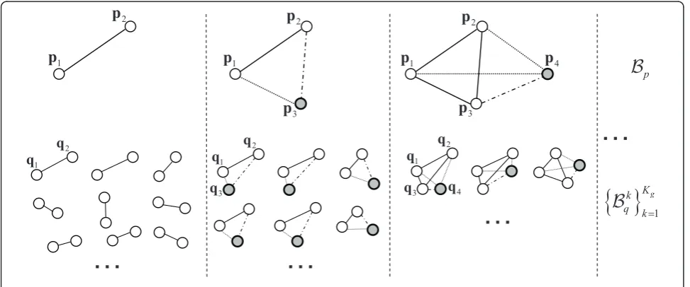
3.3 Iterative search of matchingN-points bases
Finding the best corresponding point base set of aN -points base Bp∈P requires to test O(nN) N-points
bases inQwith a blind exhaustive search, which is often impractical due to the size of the search space. To effi-ciently search approximate congruentN-points bases in Qgiven a baseBp∈P, we employ an iterative approach
that makes use of the codebook defined in the previous sections. We start by selecting a query setBicomposed
by a points pair ofBpand search candidate congruent
2-points bases usingSfandSm. We then iteratively add
points ofBptoBiand build the corresponding candidate
congruent bases by grouping point pairs or adding
single points to the previous candidate bases untilBi
corresponds to Bpand all candidate bases are
repre-sented by N-points bases. Algorithm 1 describes the procedure in detail, which is also illustrated in Figure 2. In Algorithm 1, we describe two approaches to gradually expand the size of a congruent base inQ. The first approach is to add an approximate congruent point pair having a common point with a previous base and satis-fying the used congruent constraint. The second approach is to add a single point fromMf(pi+1) accord-ing with the used congruent constraint. Since it is diffi-cult to select the best approach, we use a simple strategy based on the product of set sizes |Mf(pi)| × |Mf(pi+1)|. In particular, if this size product is large, we use the former method, otherwise the latter one.
4 RANSAC pose optimization
To find the best transformationT that aligns the two points setsP andQ, we employ a variant of the RAN-SAC algorithm [9], which is a widely used general tech-nique for robust fitting of models to data corrupted with noise and outliers. The RANSAC-based alignment procedure is straightforward: randomly pick a baseBpof
Nnon-collinear points fromP; detect the corresponding best congruent bases{Bk
q} Kg
k=1and for each one compute the candidate transformation that aligns points inBp
with points inBk
q; and finally verify the recovered
trans-formations and detect the best one using a best fit cri-teria. To achieve a certain probability of success, this procedure is repeated for different choices of bases from P. Over all such trials in all iterations, we select the best transformation T with the best fit measure. Our
…
…
…
…
p
^ `
1g K k q k
1
p
2
p
1
p
p
12
p
p
23
p
p
34
p
1
q 2 q
1
q q1
2
q q2
3
q
3
q q4
adopted RANSAC algorithm terminates when one of the following two cases is reached:
1. The number of iterations reaches a predefined maximal iteration number Imax;
2. The best transformation is not updated after Inou
continuous iterations.
Our method makes use of the codebook-based search scheme defined in Section 3, which is constructed before the optimization. The following sections describe in details each single step of the RANSAC iteration.
4.1 Random selection
Assumed kpoints inP having corresponding points in Q, the probability of successfully selecting N-points from P having correspondences inQisp(N)≈ (k/m)N, wherem= |P|. To successfully recover the transforma-tion, in general, we employ a base size N= 3, 4 or 5 points because the probability of success greatly decreases when the base sizeNincreases. Moreover, to make the estimated transformation more robust, we select theN-points baseBpfrom P as decentralized as
possible in 3-D space.
Notice that when the overlap between two scans is small only a very small subset of points inP have corre-sponding points inQ. In this case, the probability of selecting aN-points base inP with a uniform distribu-tion having a correspondingN-points base inQis very low. To improve the selection probability, we propose a probability-based RANSAC approach described as fol-lows. We initially build a m × m pairwise matching probability table Sp for all point pairs inP. Given a
point pair (pi, pj) in P, its matching probability is
defined by
Sp(pi,pj) = 1 Cexp
−ϕ1
|Mf(pi)| · |Mf(pj)| n2 −ϕ2
||pi−pj|| dqmax
−ϕ3sc((pi,pj), (q˜i,q˜))
, (14)
whereCis a normalization factor, and{ϕi}3i=1are three positive constants.(q˜i,q˜j)is the best matched point pair of (pi, pj) with the best similarity score in Equation 3.
Notice that if no approximate congruent match(q˜i,q˜j)
is found, we set the probability value to zero, i.e.,Sp(pi, pj) = 0. This probability is high if:
1. Both points pi and pj potentially have several
matches in Q based on their considered local descriptors (see Equation 12),
2. They are well spaced and
3. There exists a very similar 2-points base
(pi,pj)∈Qaccording to the similarity measuresc(·,
·) defined in Equation 3.
The selection of aN-points baseBp={psk} N
k=1from P proceeds iteratively by adding points to a selected point setBpc. This is done as follows:
1. We randomly select the first two points(ps1,ps2) based on the probability values {Sp(pi, pj)}i>j,1≤i, j≤m
of the upper triangular part of the symmetric pair-wise matching probability tableSp. These points are
added to the initially emptyBpc.
2. The next pointpsk+1, k≥2is randomly selected based on the joint probability values
psk∈Bc
pp(pi,psk)
pi∈P,pi∈Bcp .
In this way, there is a high probability to select a N -points baseBpwith corresponding points inQ.
At the end of the RANSAC iteration, if we success-fully recover a candidate transformationT using the selected N-points base, the probability table Sp is
updated. In particular, we update the corresponding ele-ments of pointspsk ∈Bpby suitably increasing the
prob-ability values: for each pointpi∈P, the new probability valueSp(pi,psk)(and its symmetric valueS
p(psk, pi))is evaluated as
Sp(pi,psk) =Sp(pi,psk)·exp(ν·fQLCP(T,δ)), (15)
where fQLCP(T,δ)is the transformation fitting criter-ion described in Sectcriter-ion 4.4 andνis a positive constant. The update of probabilities increases the chance to select good samples inP, which is very useful for align-ing two scans with a small overlap. To avoid unbalanced values inSp, we decrease the probabilities of some
ele-ments if these have been updated too frequently during the RANSAC iterations. In particular, we decrease the probability value as follows:
Sp(pi,psk) =S
p(psk,pi), =ψ·Sp(pi,psk), (16)
whereψÎ(0, 1) is a positive constant.
4.2 Approximate congruent group selection
After selecting anN-points baseBpfromP, we need to
detect a set of approximate congruentN-points bases. This is done by exploiting the fast codebook structures Sfand Sm defined in Section 3. In particular following
Algorithm 1, we are able to iteratively recover the set of congruent N-points bases as we select points ofBpfrom
P. We keep only the first Kg candidates according to
Equation 3. These KgN-points bases{Bkq} Kg
4.3 Transformation estimation
Given two point setsP andQwith overlapping regions in arbitrary initial positions, we recover the best trans-formation from a prescribed family of transtrans-formations, typically rigid transformations, that best aligns the over-lapping regions ofP andQ. In case of rigid transforma-tion, we need a base size of at least three points to uniquely determine the aligning transformation. This means that our algorithm requires at least a pair of matching 3-points bases from P andQ, respectively. In particular for any givenN-points bases pairsBpandBq,
we recover the corresponding transformationT using the closed-form solution [34].
4.4 Transformation verification
To determine the best transformation, Aiger et al. [8] employ a best fitcriteria called as the largest common pointset (LCP) measure fLCP(T,δ), which refers to the transformation bringing the maximum number of points fromP to within someδ-distance of points inQ. Unfor-tunately, this criteria completely depends on the choice of the distance thresholdδ. On one hand, if this thresh-old is too large wrong transformations may result in large LCP measure values. On the other hand, ifδis too small in some cases no transformation can be found.
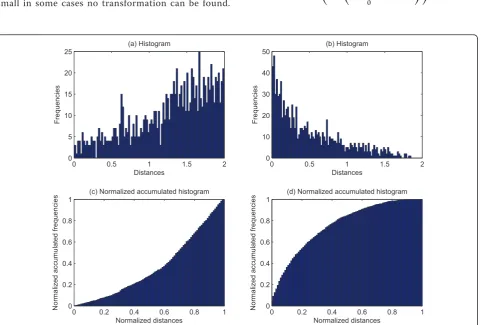
The main problem is that the LCP measure only consid-ers the quantity of matched points in overlapping regions, but not their matching quality. To solve this problem to some extent, we propose to integrate a sui-table matching quality measure into the LCP measure. Suppose that we have two transformations TaandTb
computed from two different selectedN-points congru-ent group pairs and resulting in the same LCP measure under the same distance threshold δ. Assume that the histograms of the point distances of the two transforma-tions correspond to the ones shown in Figure 3a, b, respectively. Intuitively,Tbis a better solution thanTa
because most of the corresponding point pairs have shorter distances in Figure 3b than in Figure 3a, i.e., the mean distance of the corresponding point pairs in Fig-ure 3b is smaller than that in FigFig-ure 3a. We expect that better point matches (with shorter distances) result in a better transformation. We, thus, define a suitable match-ing score based on a normalized accumulated histogram Hn(T,δ)(see Figure 3c, d) corresponding to some given transformationT as follows:
ms(T,δ) = exp ⎛ ⎝−λ
⎛ ⎝1−
1
0
Hn(T,δ) ⎞ ⎠ ⎞
⎠, (17)
0 0.5 1 1.5 2
0 5 10 15 20
25 (a) Histogram
Distances
Frequencies
0 0.5 1 1.5 2
0 10 20 30 40
50 (b) Histogram
Distances
Frequencies
0 0.2 0.4 0.6 0.8 1 0
0.2 0.4 0.6 0.8
1 (c) Normalized accumulated histogram
Normalized distances
Normalized accumulated frequencies 00 0.2 0.4 0.6 0.8 1
0.2 0.4 0.6 0.8
1 (d) Normalized accumulated histogram
Normalized distances
Normalized accumulated frequencies
where l is a positive parameter and 01Hn(T,δ)
denotes the integral ofHn(T,δ), i.e., the area below the
cumulative curve in Hn(T,δ). We use a quality-based
LCP (QLCP) measure defined by
fQLCP(T,δ) =ms(T,δ)·fLCP(T,δ)as our best fit criteria. By weighting fLCP(T,δ) with the quality estimate ms(T,δ)the QLCP measure is made less sensitive to the choice ofδthan the LCP measure.
After thetransformation estimation step we evaluate each recovered transformationTkbetweenBpandBkqw.
r.t. the mean alignment error. In particular, we test whether the error N1
pi∈Bp,qkl∈Bkq||T
kpi−qki||2 is less
than some predefined threshold, whereTkpidenotes the
transformed point of pivia Tk. We further verify each
remaining transformation by detecting how many points inPhave correspondences inQunderTkand then
mea-suring the matching score as described in Equation 17. We say that one point p∈P have a corresponding point inQunderTk, if there exists some point inQ
clo-ser withinδ-distance to the transformed point Tkp, i.e.,
∃q∈Q||q−Tkp|| ≤δ. For efficiency, we use the
approxi-mate nearest neighbours [33] for neighbourhood query-ing in ℝ3. We first select a fixed number of points {pi} ∈P and apply the transformationTk. Then, for each
transformed pointTkpiwe query the nearest neighbour
inQ. If enough points of {pi} are matched, we perform a
similar tests for the remaining points inP and assign to Tka score based on our used QLCP measure.
Finally, we update the current best transformation found with the best QLCP measure and start the next RANSAC iteration.
5 Point sampling approaches
Given two large point setsPandQ, matching approxi-matively congruent sets of points over the entire data set is not feasible. Thus, we need efficient point sampling strategies to quickly search corresponding sets and to effectively estimate and verify their transformation on a limited number of meaningful candidates points. The reliability of the proposed registration approach depends, to some extent, on the used sampling strategy. If we sam-ple too many points from scarcely meaningful regions the registration might converge slowly, find the wrong transformation (such as solutions showing sliding effects produced by samples poorly constraining the transforma-tion), or even diverge, especially in the presence of noise and outliers. Several point sampling techniques for point cloud alignment were recently proposed [6,35-37]. In [6] the random, uniform (over the surface area of a model) and normal-space sampling are considered to evaluate the convergence of the ICP algorithm. The normal-space sampling algorithm tries to uniformly spread the normals
of the selected points on the sphere of directions. The aim is to consider points that sufficiently constrain the estimated rigid transformation and improve the align-ment quality by reducing surface sliding effects. Gelfand et al. [35] proposed a variant of this algorithm to make the transformation estimation geometrically stable by selecting points that reduce both translational and rota-tional uncertainties in the ICP algorithm. This technique samples points in order to equally constrain all eigenvec-tors of the covariance matrix estimated from the points and the normals of the overlapping region of two point clouds. A similar approach was used in [36] to conceive a probability function to guide the selection of stable sam-ple points, which are also constrained by specific features. Torsello et al. [37] proposed a sampling technique to select feature points with high-local distinctiveness, which is inversely proportional to the average local radius of curvature and related to the area formed by similar points in the neighbourhood of each point. Nehab and Shilane [38] discussed the limitation of the area-based uniform sampling, where the probability of a surface point being sampled is equal for all surface points. This type of sampling might produce points very closed to each other and miss important surface features, which could successfully constrain the transformation. To over-come these drawbacks they proposed a stratified point sampling strategy ensuring an even distribution of the sample points on all surface, which implies a higher probability to catch important surface regions. This algo-rithm uses the voxelization of the model to generate ran-dom samples with controlled intra-distances. Other sampling strategies providing with uniform distribution of sample points on a surface are based on the farthest point [39] and Poisson disk sampling [40], which require the computation of geodesic distances.
In this section, we investigate four sampling approaches: random, uniform, probabilistic and com-bined sampling, which are described in details in the following.
5.1 Random sampling
Random sampling is the simplest and widely used sam-pling technique. In random samsam-pling, each item or ele-ment of the population has an equal chance of being selected at each draw. A sample is random if the method for obtaining the sample meets the criterion of random-ness (each element having an equal chance at each draw). The actual composition of the sample itself does not determine whether or not it was a random sample.
5.2 Uniform sampling
sets have similar point densities. If the acquired surfaces present similar point densities, the above mentioned ran-dom sampling deserves to be an acceptable choice, which will also result in similar point densities in the sampled overlapping parts. However, this assumption does not hold in general. Point density depends on the distances and on the incident angles of the scanned surfaces with respect to the scanner sensor position and orientation, respectively. Normally, short distances and small incident angles lead to surfaces with high-point densities and accuracies, which we consider as high-resolution regions. Random sampling does not guarantee an equal spread of the generated points neither on the surface nor in the volume of the scanned model, and can sample points very close to each other. Thus, it is more likely that it misses important surface features than an evenly distributed sam-pling [38]. This effect is particularly evident in case of scanned data with non-uniform point densities.
Many approaches to perform a sampling of uniformly distributed points on the model surface can be employed [38-40]. We propose a simple and efficient variant of the method presented in [38], which is based on cubic voxeli-zation of point clouds and that provides with samples evenly displaced on typical scanned surfaces. Given a point setP, we can assign them into a set of 3-D cubic voxels of equal sizes, which partition the 3-D space. For each such voxel, we select the closest point to the voxel center as the sampled point. To obtain a sampled point set of a given sizeNs, we start by splitting the minimal
bounding box of the point cloud into a small set of 3-D cubic voxels. We then iteratively split each voxel into eight small voxels until there are enough sampled points found. With this strategy, however, we cannot obtain an accurately fixed-size set of sampled points since most of the voxels do not contain points. LetNlbe the number of
sampled points at thelth level. The final levelLis such that its number of pointsNLis not less thanNsand the
number of points at the previous level isNL-1< Ns. To
obtain a sampling of the expected sizeNs, the simple way
is to randomly selectNspoints from theNLpoints of the
Llevel. To achieve a more uniform distribution, we pro-pose, instead, to re-split all points inP into a set of cubic
voxels of size 8N2 s NL−1NL
1 3
SL−1, where SL-1 denotes the
voxel size at the (L -1)th level. In this way, the number of uniformly sampled points is very close toNs, but still
not exact. If the number is larger thanNs, we randomly
selectNspoints from them. Otherwise, we add some new
points from sampled point set at theLth level.
5.3 Probabilistic sampling
If the acquired surfaces are very similar in structure, e.g., the surfaces of an indoor environment composed of a
main flat wall and several small objects in the front of it, the above two sampling approaches may not be efficient for our proposed registration. One reason is that we select the best transformation based on the degree of overlap in the point sets, but not based on the whole scene structure. In the above example, points from the main single wall weakly constrain translations and generate sliding effects in the final alignment, as already discussed in [6,35-37]. Another reason is that a selectedN-points base from the wall would have a large number of approximate congruent bases. This would require expensive searches, tests, esti-mates and verifications of candidate transformations over a large set of approximate congruent bases. To avoid these problems, we expect to consider more points from objects in front of the wall, which would reduce the computation and better constrain the rigid transformation. Similarly to [37], this is achieved by utilizing a probabilistic sampling technique, which selects points based on their likelihoods computed from a specific weight function. The weight function determines how much each point is relevant for registration and is basically associated with the local geo-metrical properties of the surface at each point. We experimented with two different weight functionsωSVand ωAPD based on surface variation and adjacent point
dis-tance, respectively.
Thesurface variationof a pointpis defined as:
ωSV(p) =
3λ1
λ1+λ2+λ3
, (18)
wherel1 ≤l2 ≤l3 are the eigenvalues corresponding
to the principal components of a set ofkpoints in the neighbourhood of p. ωSV(p) Î [0, 1] indicates how
much the surface atplocally deviates from the tangent plane [41]. In practice,ωSV(p) roughly approximates the
mean curvature atp: when its value is close to zero it indicates that the surface is locally planar, while, when ωSV(p) is large, p identifies an interesting feature like
corners, bumps, etc.
Theadjacent point distance[42] is defined by exploit-ing the grid structure of range image I related to the acquired point cloud. Let pbe a valid point associated with a pixel of I, its adjacent point distanceAd(p)is defined as the median of the distances between p and its adjacent valid pointspkin a 3 × 3 neighbourhood of p, i.e., Ad(p) = mediank||p−pk||. Then, to reduce the
effect of measurement noise, a median filter of size 5 × 5 is applied on the resulting adjacent point distance map Ad to get a filtered mapA˜d. The weight function ωAPDof a pointpis then defined as:
ωAPD(p) =
ˆ A2
d ifAˆd(p)≥ ˆAd,
ˆ
Ad(x)2otherwise.
whereAˆddenotes the 95th percentile of the adjacent point distances in an ascending order of all points in
˜
Ad. The use of Aˆd effectively suppresses estimation
errors from outliers. ωAPD(p) estimates the local
sam-pling sparsity of the scanned surface atp. High values of ωAPDcharacterize those points having a
neighbour-hood sparsely sampled, typical of corner and edge points and regions scanned with low incident angle, which are likely located in the overlapping area of the models.
5.4 Coupled sampling
Besides the aforementioned three sampling approaches, we also consider to couple different sampling approaches in some order. For example, a point set P1 is selected from the initial point set P based on prob-abilistic sampling, after that, another point set P2is selected fromP1based on uniform sampling. The finally sampled point set can be selected from the initial point set P via two or more sampling in some order with given sampling ratios. The sampling ratios of the finally sampled point set PSfrom P via Ssampling processes
are denoted as |P1| : |P2| :· · ·: |PS| where | · |
denotes the set size. For different scans to be aligned, we can select a suitable sampling approach.
6 Integrating texture features
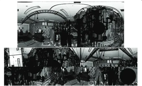
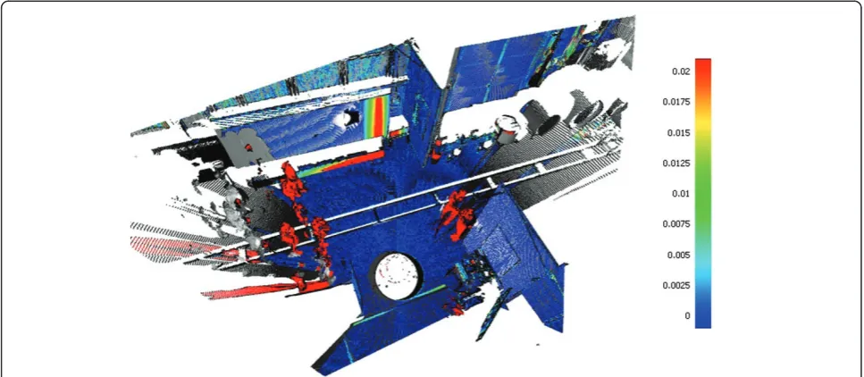
If the acquired models lack geometric details to be used as good anchor points for correct registration, we can still employ features extracted from other visual sources provided by the laser range scanners, e.g., the reflectance image. Laser range scanners are non-contact 3-D scan-ners that measure the distance from the sensor to points in the scene, typically in a regular grid pattern. A nat-ural byproduct of this acquisition process is the reflec-tance image. A reflectance image (shown in Figure 4) stores in each pixel the portion of laser light reflected from the corresponding surface point, providing with important information about its texture. Both 3-D space distribution and texture characteristics of the texture features extracted from the reflectance images can well constrain a rigid transformation in 3-D space. As shown in [11,12] texture features can be effectively used to identify anchor points leading to a well-constrained rigid transformation.
A feature is accompanied by a descriptor, which locally and compactly describes the texture around the feature pixel. In our application, we are interested in good local feature descriptors, which should have a high-local distinctiveness, invariant w.r.t. affine
transformations, and possibly robust w.r.t. illumination changes and local deformation. Several local feature descriptors were presented in the literature [32,43]. Among them, the most suitable for our application are the SIFT [44], SURF [45] and FAST [46] descriptors, which we extract from the reflectance images of our scanned models and consider as relevant sample points to be matched by our registration algorithm.
6.1 Reflectance image rectification
The aforementioned features cannot be efficiently extracted directly from the reflectance image associated with a scanned model, since its intrinsic spherical for-mat strongly affects the quality of their descriptors, which are not designed to be robust w.r.t. spherical dis-tortions. Indeed, typical laser scanner acquisition sys-tems are usually composed by a fixed platform and a rotating head, which are naturally modelled by simple spherical projections. The resulting acquired images are then obtained by mapping spherical images onto single image planes. The meridians of a spherical image are mapped to vertical viewing planes, and the parallels are mapped to viewing cones with the vertex in the sensor position.
In order to reduce the distortion induced by the sphe-rical projection, we compute the above mentioned fea-ture descriptors on an atlas of rectified images (shown in Figure 4). This is possible since both the spherical projection and the atlas perspective projections will share the same point of view.
To recover the set of rectified images, we initially select a field of view valueafov(in our experimentsafov
= 60°). We then calculate the widthwr and heighthr of
each rectified image by constraining the pixel resolution to the resolution of the spherical image equator, i.e., the width ws of the spherical image :wr=hr=ws·360αfovo. Given the pixel dimensions of the image plane, we define a standard perspective projection whose principal point is represented by the central pixel of the image plane. The only missing intrinsic parameter, the projec-tion focus, can be easily recovered givenafov, wrandhr.
To determine the extrinsic parameters of each projec-tion, we fix the camera point of view to the spherical projection point of view, i.e., the local origin of the point cloud. We then sample the sphere with vequally distributed directions. The value of vdepends on the required field of view and is estimated such that the images contained in the atlas completely cover the initial spherical image. Given the camera directiondiwe
recover the remaining extrinsic parameters of the ith image aligning the camera principal direction to diand
the vertical direction with the vertical direction of the spherical image. Exploiting each projection matrix, we
can associate to each final image pixel its corresponding viewing ray, and from this the pixel’s corresponding coordinates in the original spherical image. These corre-spondences are used to perform a bilinear interpolation of the spherical image to recover each single finally rec-tified image (see Figure 4).
The atlas generation only depends on the field of view used. Small values generate multiple small images, whereas large values generate fewer images but with higher-perspective distortions.
6.2 Texture features extraction and integration
From the original reflectance image or the atlas of recti-fied images generated from a reflectance image, we extract a set of texture features for registration by using the following methods:
1. SIFT [44]: this feature descriptor encodes the trend of the image local gradient around a pixel as a histo-gram of typically 128 bins. This descriptor is invariant w.r.t. scaling and rigid 2-D transformation and robust w.r.t. affine distortion, addition of noise, and change in illumination. This descriptor is very accurate in identifying relevant interest point, but its computa-tion is usually slow without exploiting the GPU [47]. 2. SURF [45]: this method efficiently detects features by computing a rough approximation of the Hessian matrix using integral images. The resulting descrip-tor is based on sums of approximated 2-D Haar wavelet responses, which is more compact and much faster to compute than the SIFT descriptor. 3. FAST [48]: this techniques classifies a pixel as corner if there is a sufficiently large set of relevantly brighter (darker) pixels in a circular pixel neighbour-hood of fixed radius. This feature detection algo-rithm is very fast, up to 30 times faster than the SIFT one, but is not invariant w.r.t. scaling and does not provide with effective descriptors [43], which are usually computed by using other techniques (e.g., with the SURF method in this paper).
4. Harris corner detector [49]: it has been widely used in image processing and computer vision, and computes corner features by analysing the local changes of the image intensity with patches shifted by a small amount in different directions. It is not scale and affine invariant, and usually generates a high number of features.
7 Experimental results
7.1 Test data and evaluation criteria
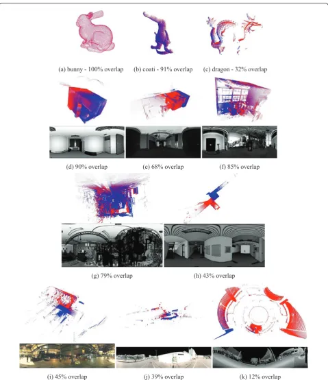
We tested our point-based registration algorithm on a variety of input data with varying amount of noise, out-liers, and extent of overlap. Our test dataset includes some small object models as shown in Figure 5a, b, c, which are selected from the data provided in the demo application of the 4PCS algorithm [8]b. Other test data are models of large indoor/outdoor scenes acquired by different types of scanners, which are mostly selected from [20], as shown in Figure 5d, e, f, g, h, i, j, k. In total, we tested 11 pairs of scans with different extents of overlap as shown in Figure 5. These 11 pairs of scans are noted by {Gn}n=a,...,k corresponding to the models shown in Figure 5a, b, c, d, e, f, g, h, i, j, k, respectively. The small objects models inGa−Gcconsist of around 20,000-30,000 points. Indoor scan data(Gd−Gi)were captured by Z+F IMAGER 5003/5006/5006i laser range-scanners. Outdoor scan data (GjandGk) were captured by the RIEGL LMS-Z420i laser range-scanner. The accuracy of a point acquired by the Z+F IMAGER 5003 (5006 and 5006i) laser scanner is 3 mm (1 mm) along the laser-beam direction at a maximal distance of 50 m from the scanner. The accuracy of the RIEGL LMS-Z420i laser scanner is 10 mm at 50 m. The resolution of all indoor scans is about 2, 530 × 1, 080 and the reso-lution of all outdoor scans is 3, 000 × 666. No surface normals were provided for points in the scan dataGa,Gb andGc. For the other scans, we always employed the surface normals into our registration algorithm. The scan data inGa−Gc were scaled so that the bounding box diagonal lengths of the first scans in these scan pairs are taken as 100 units. The bounding box diagonal lengths of the first scans of other eight scan pairs Gd−Gk are around 10, 28, 26, 37, 77, 142, 1, 860, and 398m, respectively. The overlap rates shown in Figure 5 were computed as follows. The overlap rate of two
point sets P and Q is defined as
o(P,Q) = min|P|P∈Q||,|Q|Q∈P||, where|·|denotes the size of a point set andP ∈Qdenotes a subset ofP in which for each point there exist at least one point inQwhose dis-tance to it is below a given threshold. To produce a rea-sonable overlap rate in 3-D space, we compute the overlap rate by using large point subsets selected from P andQusing our voxel-based uniform sampler instead of using original point sets. Our registration algorithm was implemented in C++ on a Windows XP system and integrated into our commercial softwareJRC 3-D Recon-structor. All experiments were executed on a 2.67 GHz Intel machine.
We fixed the poses of all reference scans (i.e.,{Q}) to an identity rotation matrix and no translation. To evalu-ate the transformation estimation accuracy of our
registration algorithm, we first employed our algorithm on all tested pairs of scans to recover a good initial transformation for each scan pair and then applied the ICP optimization algorithm [5] to get a well-aligned transformation. We observed that the mean residual error after the ICP registration optimization was always comparable with the laser scanner measurement error, which is much lower than the estimation errors of our proposed N-points congruent sets (NPCS) registration algorithm. For this reason, we regarded this ICP-opti-mized transformation as the ground truth transforma-tion Tg for evaluation. Thus, given an estimated
transformationT fromP toQ, the estimation error is defined as the median of the point distances after apply-ingT andTgontoP, i.e.,medianp∈P||Tp−Tgp||.
The transformation estimation accuracy was statisti-cally evaluated by running our registration algorithm Nrun = 20 times on each tested pair of scans. In each
run, we refresh the input data by setting a random pose for the moving scan followed by re-sampling. For each scan pair, we set a suitable maximal estimation error
Δmaxin advance. If the estimation error was aboveΔmax,
we considered it as failed. The maximal estimation errors were set asΔmax= 5 units,Δmax= 1 m,Δmax= 2
m andΔmax = 5 m for small object modelsGa−Gc, the
indoor modelsGd −Gh, the large indoor modelsGiand the outdoor modelsGj −Gk, respectively. Based on the numberNsucof successful estimations and the number
Nrun of runs the following three indicators were then
used to evaluate our method: (1) the successful estima-tion rate Sr= NNrunsuc to evaluate its robustness; (2) the
median estimation error Δ among allNsuc successful
estimations to evaluate its accuracy; (3) themedian esti-mation time t over all Nrun runs to evaluate its
effi-ciency. Note that the estimation time does not include pre-processing computation time (i.e., texture feature detection/matching, point sampling, etc), but it incorpo-rates the codebook building time, which took <1 s with the basic RANSAC and around two seconds with the probabilistic RANSAC using our parameter setting. The feature detectors listed by increasing processing time are Harris, FAST, SURF and SIFT. The point sampling approaches listed by increasing processing time are ran-dom, probabilistic and uniform samplings.
7.2 Performance evaluation
The performance of our proposed NPCS registration algorithm was evaluated on the aforementioned test data. The main parameters were set as follows. We employed congruent points sets of sizeN= 4. The two main parameters for searching best N-points congruent sets in Algorithm 1 were set asKp= 2, 000 andKg= 50.
(a) bunny - 100% overlap (b) coati - 91% overlap (c) dragon - 32% overlap
(d) 90% overlap (e) 68% overlap (f) 85% overlap
(g) 79% overlap (h) 43% overlap
(i) 45% overlap (j) 39% overlap (k) 12% overlap
proposed QLCP measure in Equation 17. Given two point setsP andQ, we tried to recover the transforma-tion from P (moving point set) toQ(reference point set). We selected 500 points fromP and 1,000 points fromQfor searching N-points congruent sets between them. However, for transformation verification, we selected larger subsets, i.e., 1,000 points from P and 2,000 points fromQ. This allows the estimation of a more accurate and robust transformation. The voxel-based uniform sampling approach was used to select these points. Our registration algorithm always used the surface normals of points when provided. The maximal normal deviation for the corresponding point pairs was set to 30°. In our experiments, we used the RANSAC-based approach by setting Imax= 1, 000 andInou= 200,
which are the allowed maximal iteration number and the continuous iteration number in which no better transformation was found, respectively. The estimation errors of the first three scan pairsGa−Gc were reported in canonical units (i.e., 100 units are equal to the bounding box diagonal lengths), while those of the other eight scan pairsGd−Gk in meters. Notice that the same parameter values were used in all experiments described below, unless clearly stated otherwise for particular experiments.
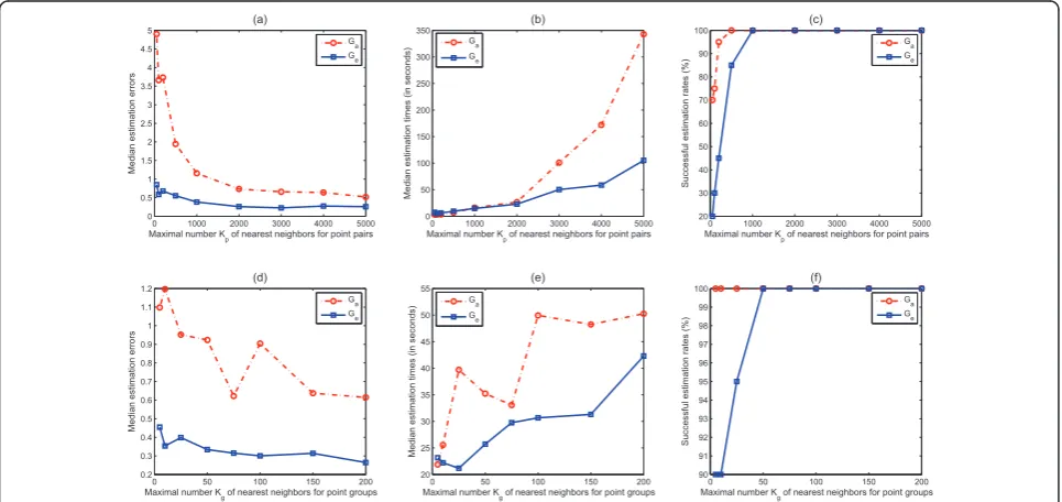
Figure 6 shows the performance comparison of our NPCS algorithm with different KpandKgon three scan
pairsGa,GeandGi. First, we fixedKg= 50 and tested the
effects of differentKpon the registration accuracy
(med-ian estimation errors), efficiency (med(med-ian estimation times) and robustness (successful estimation rates), as
shown in Figure 6a, b, c, respectively. We can observe that larger values ofKp led to an improvement of the
registration accuracy and robustness, but also required longer execution times. In Figure 6c, we can notice that 100% successful estimation rates were achieved for all tested scan pairs whenKp≥1, 000. Second, we fixedKp
= 2, 000 and tested the effects of different Kgon
regis-tration performance shown in Figure 6d, e, f. The varia-tion ofKgresults in similar effects as forKp. WhenKg≥
50, the successful estimation rates were always Sr =
100% for all tested scan pairs.
Table 1 illustrates the performance evaluation of our NPCS algorithm on three scan pairsGc,GdandGjwhen the sizeNof congruent point sets was set asN= 3, ..., 6, respectively. As explained before, large values ofN(≥ 6) result in a low probability of successfully selectingN -points congruent sets between two point sets and in longer estimation times. Small values ofN (= 3) led to an increase of the candidateN-points congruent sets in QgivenNpoints inP, but sometimes the matched sets found are not enough to well constraint the transforma-tion and the algorithm falls into local minima.
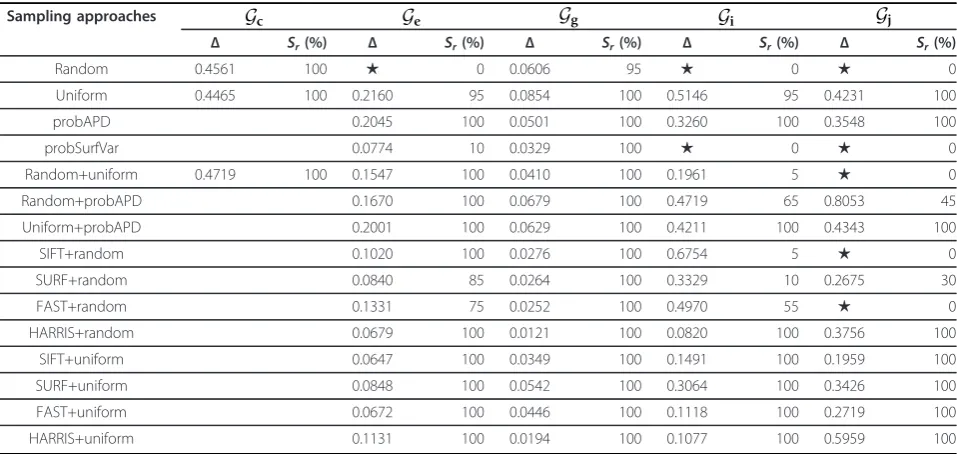
The performance comparison of different sampling approaches on five scan pairs is shown in Table 2. In this experiment, we tested the following sampling strate-gies: the random sampling; the voxel-based uniform sampling; two probabilistic sampling approaches ( pro-bAPD-based on adjacent point distances, probSurfVar -based on surface variations); four texture feature--based sampling using the SIFT, SURF, FAST and HARRIS fea-ture detectors as samplers. Some sampling strategies
0 1000 2000 3000 4000 5000 0 0.5 1 1.5 2 2.5 3 3.5 4 4.5 5
Maximal number Kp of nearest neighbors for point pairs
Median estimation errors
(a)
Ga Ge
0 1000 2000 3000 4000 5000 0 50 100 150 200 250 300 350
Maximal number Kp of nearest neighbors for point pairs
Median estimation times (in seconds)
(b) Ga Ge
0 1000 2000 3000 4000 5000 20 30 40 50 60 70 80 90 100
Maximal number Kp of nearest neighbors for point pairs
Successful estimation rates (%)
(c)
Ga Ge
0 50 100 150 200 0.2 0.3 0.4 0.5 0.6 0.7 0.8 0.9 1 1.1 1.2
Maximal number Kg of nearest neighbors for point groups
Median estimation errors
(d)
Ga Ge
0 50 100 150 200 20 25 30 35 40 45 50 55
Maximal number Kg of nearest neighbors for point groups
Median estimation times (in seconds)
(e) Ga Ge
0 50 100 150 200 90 91 92 93 94 95 96 97 98 99 100
Maximal number Kg of nearest neighbors for point groups
Successful estimation rates (%)
(f)
Ga Ge
were coupled and reported in Table 2 combined with the character ‘+’. For instance, the coupled sampling
“random+uniform”denotes that we first applied the ran-dom sampling to get a point subsetP1from the initial point setP and then applied the uniform sampling to get the final point subset P2from P1. Here, the sam-pling ratios of all coupled samsam-pling approaches were set to P2:P1= 0.5. All texture feature-based sampling methods were coupled with random or uniform pling. From Table 2, we observe that the uniform sam-pling performs better than the random samsam-pling both when is considered alone and when is coupled with other sampling strategies, i.e., with the probAPD-based sampling and feature detectors. Among the probabilistic sampling methods the probAPD-based sampling resulted to be a very good choice if available, since it relevantly improved the registration robustness and also increased its accuracy. On the contrary, the probSurf-Var-based sampling showed lack of robustness, but worked very well for models rich of geometric features, which were captured from geometrically complex
scenes, as those inGg. In some scenes, texture feature detectors turned out to be a good first sampler. In those cases, they improved the transformation accuracy as shown by ‘FAST+uniform” inGe( = 0.0672 m)and by
“HARRIS+random” in Gg( = 0.0121 m) and Gi( = 0.0820 m). Among the texture feature-based sampling “SIFT+uniform” and“FAST+uniform” also demonstrated a very good robustness by always scoring Sr = 100% as the probAPD-based sampling, but with
improved accuracies for all models apart from those in Gj. Notice that if it is not possible to extract enough tex-ture featex-tures the remaining points were selected by the following coupled sampling approach.
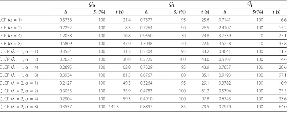
Our employed QLCP measure for verifying the esti-mated transformation depends on two main parameters, i.e., lin Equation 17 and δ-distance. In this paper, we computedδ=αd˙vref, whereais a positive constant and ˙
dvref= medianq∈Qv||q−nc(q)||, where Qv ⊂Q
repre-sents the set of points used for transformation verifica-tion and nc(q) denotes the closest point of q inQv.
Table 3 shows the comparison of our NPCS algorithm when using the LCP or the QLCP measure with differ-ent parameters on three scan pairs: Gb, Gi, andGj. In practice, the LCP measure corresponds to the QLCP measure withl= 0. From Table 3, we observe that our proposed QLCP measure led to higher successful esti-mation rates and more accurate transforesti-mations than the LCP one. In addition, notice that a largel slightly increased the estimation robustness when a largeawas used. In the rest of the experiments reported in the paper, we usedl= 1 anda = 2.
Table 1 Performance evaluation of our NPCS algorithm with different sizesNof congruent point sets
N Gc Gd Gj
Δ Sr(%) t(s) Δ Sr(%) t(s) Δ Sr(%) t(s)
3 0.7060 100 61.5 0.0770 100 29.4 0.5903 100 18.5
4 0.3906 100 35.1 0.0508 100 45.4 0.7819 100 16.6
5 0.4532 100 39.2 0.0484 100 53.9 0.6114 100 20.6
6 0.4277 100 40.8 0.0462 100 90.6 0.9586 95 77.1
Table 2 Performance evaluation of different sampling approaches on five pairs of scans
Sampling approaches Gc Ge Gg Gi Gj
Δ Sr(%) Δ Sr(%) Δ Sr(%) Δ Sr(%) Δ Sr(%)
Random 0.4561 100 ★ 0 0.0606 95 ★ 0 ★ 0
Uniform 0.4465 100 0.2160 95 0.0854 100 0.5146 95 0.4231 100
probAPD 0.2045 100 0.0501 100 0.3260 100 0.3548 100
probSurfVar 0.0774 10 0.0329 100 ★ 0 ★ 0
Random+uniform 0.4719 100 0.1547 100 0.0410 100 0.1961 5 ★ 0
Random+probAPD 0.1670 100 0.0679 100 0.4719 65 0.8053 45
Uniform+probAPD 0.2001 100 0.0629 100 0.4211 100 0.4343 100
SIFT+random 0.1020 100 0.0276 100 0.6754 5 ★ 0
SURF+random 0.0840 85 0.0264 100 0.3329 10 0.2675 30
FAST+random 0.1331 75 0.0252 100 0.4970 55 ★ 0
HARRIS+random 0.0679 100 0.0121 100 0.0820 100 0.3756 100
SIFT+uniform 0.0647 100 0.0349 100 0.1491 100 0.1959 100
SURF+uniform 0.0848 100 0.0542 100 0.3064 100 0.3426 100
FAST+uniform 0.0672 100 0.0446 100 0.1118 100 0.2719 100
HARRIS+uniform 0.1131 100 0.0194 100 0.1077 100 0.5959 100
The integration of scene structure information to our NPCS algorithm can greatly reduce the estimation time, as described in Section 2 and illustrated in Table 4. This can also slightly improve the accuracy of the recovered transformation. Here, the scans inGdandGf were auto-matically classified as orthogonal scenes.
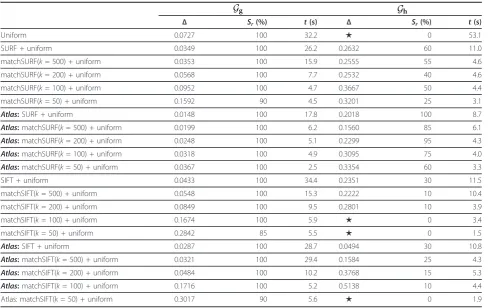
Table 5 shows the performance evaluation of our