Volume 2010, Article ID 923748,13pages doi:10.1155/2010/923748
Research Article
An Interactive Procedure to Preserve the Desired Edges during
the Image Processing of Noise Reduction
Chih-Yu Hsu,
1Hsuan-Yu Huang,
2and Lin-Tsang Lee
21Department of Information and Communication Engineering, ChaoYang University of Technology, Taichung 41349, Taiwan 2Department of Applied Mathematics, National Chung-Hsing University, Taichung 40227, Taiwan
Correspondence should be addressed to Chih-Yu Hsu,[email protected]
Received 1 December 2009; Revised 5 February 2010; Accepted 30 March 2010
Academic Editor: Yingzi Du
Copyright © 2010 Chih-Yu Hsu et al. This is an open access article distributed under the Creative Commons Attribution License, which permits unrestricted use, distribution, and reproduction in any medium, provided the original work is properly cited.
The paper propose a new procedure including four stages in order to preserve the desired edges during the image processing of noise reduction. A denoised image can be obtained from a noisy image at the first stage of the procedure. At the second stage, an edge map can be obtained by the Canny edge detector to find the edges of the object contours. Manual modification of an edge map at the third stage is optional to capture all the desired edges of the object contours. At the final stage, a new method called Edge Preserved Inhomogeneous Diffusion Equation (EPIDE) is used to smooth the noisy images or the previously denoised image at the first stage for achieving the edge preservation. The Optical Character Recognition (OCR) results in the experiments show that the proposed procedure has the best recognition result because of the capability of edge preservation.
1. Introduction
Digital images are noisy due to environmental disturbances. To ensure image quality, image processing of noise reduction is a very important step before analysis or using images. Optical Character Recognition (OCR) system is an example that is very sensitive to noise. The quality of documents influences the results of recognition. Image noise decreases the accuracy of the recognition of documentations by OCR (optical character recognition) software because of blurred edges. Great damage will be caused in defense and security applications when OCR software is used for the scanning and recognition of documents such as passports and ID cards in busy airports where speed and accuracy are critical for processing thousands of documents daily. The most important image processing technique for noise reduction is the image denoising method. The purpose of image denoising method is to increase signal-to-noise ratio (SNR) in an image. However noise reduction always induces blurred edges by an image denoising process. Development for edge-preserved image denoising method is necessary for OCR software. The paper is to develop a denoising procedure with the edge preservation capability. The OCR system is a research field in pattern recognition [1, 2] and is used to convert papers, books, and documents into electronic
files [3]. Researchers developed several methods in order to remove these image noise including Gaussian noise, salt and pepper noise [4]. There are some image filters, which are used for image denoising [5,6] and the Gaussian filter is a well-known one [7]. In the period between 1984 and 1987, Koenderink and Hummel showed how Gaussian filters removed noise that was equal to dispersion effects of the isotropic diffusion equation, so Gaussian filters are called Diffusion Filters.
(a)
0 50 100 150 200
0 50 100 150 200 250 (b)
Figure1: (a) Synthetic image and (b) the grayscale value of the 36th row of (a).
0 50 100 150 200
0 50 100 150 200 250 A1 β1 α1 (a)
0 50 100 150 200
0 50 100 150 200 250 A2 β2 α2 (b)
0 50 100 150 200
0 50 100 150 200 250 A1 β1 α1 A2 β2 α2 (c)
Figure2: (a) The front of signal ofFigure 1(b), (b) the back of signal ofFigure 1(b), and (c) the signal is superimposed by (a) and ( b).
In this paper, we propose a new procedure including four stages. At the first stage of the procedure, any kind of denoising algorithm can be applied on an original noisy image to get a well-denoised image. At the second stage, an edge map can be obtained to find the edges of the object contours by the Canny edge detector applied on the previously denoised image at the first stage. Since the contour edges are not found completely, then the users maybe need interactively modify the edge map to keep the edges of the desired object contours. At the third stage, manually modify the edges of edge map to match the desired edges. At the final stage, a new method Edge Preserved Inhomogeneous Diffusion Equation is used to smooth the original noisy image or the previously denoised image at the first stage and achieve preserving desired edge. The proposed procedure has the edge preservation capability that makes OCR results the best in this experiment.
2. Mathematic Formulation
Section 2.1introduces the digital image as a matrix, and one row can be considered as a signal.Section 2.2introduces how to find the solutions of a one-dimensional inhomogeneous diffusion equation by using Fourier series.Section 2.3 pro-posed a flow chart of the EPIDE denoising method.
2.1. Digital Images and Signals. We defined am×ngrayscale digital image as a functionu(x,y). The value of the function
u(x,y) is an image intensity that is between 0 and 255. For a gray image, the functionuhas grayscale values of image pixels. The coordinates (x,y) are locations of the pixels in an image. The grayscale values of theith row ofu(x,y) are denoted byu(i, 1 : n) which can be considered as a one-dimensional signal with length n. For example, the red line as shown inFigure 1(a)is the 36th row of the image. As shown inFigure 1(b), the grayscale values profile is composed of two Box functions.
2.1.1. One-Dimensional Signals. One-dimensional signals can be considered as piecewise constant functions, Heaviside function is suitable to discrete piecewise constant functions [11]. Heaviside functionH(x) is defined as:
H(x)=
0, x <0,
1, x >0. (1)
The Heaviside functionH(x) is discontinuous atx =0, and the value is usually defined by 1/2 at x = 0. If the Heaviside functionH(x) is shifteda, then Heaviside function isH(x−a). Box Functionφcan be represented by Heaviside functionH(x) asφ(x)=(H(x)−H(x−1)). The Box function can be represented as follows:
φ(x)=
1, 0< x <1,
0 50 100 150 200 0 50 100 150 200 250 (a)
0 50 100 150 200
0 50 100 150 200 250 (b)
0 50 100 150 200
0 50 100 150 200 250 (c)
Figure3: (a) The grayscale value of the 36th row ofFigure 1(a), (b) the Fourier series with 300 terms, and (c) diffused result by diffusion equation att=3.
−3 −2 −1 0 1 2 3
3.5
3
2.5
2
1.5
1
0.5
0 ×105
(a)
−3 −2 −1 0 1 2 3
8 6 4 2 0 −2 −4 −6 −8 ×10⁻⁴
(b)
Figure4: (a)δ(x)=(ε/π)/(x2+ε2),ε=10−6and (b)δ(x)= −2εx/π(x2+ε2)2,ε=10−6.
As shown inFigure 1(b), the 36th row ofu(x,y) isu(36, 1 :n) and the profile of the row is represented by two Box functions as in the following equation:
u(36, 1 :n)=
2
k=1
Ak
H(x−αk)−Hx−βk
. (3)
One signal can be superimposed by two signals. Figure 2 shows how to use two box functions to superimpose the signal inFigure 1(b).
If there are M Box functions in the ith row ofu(x,y), the profile ofu(i, 1 :n) can be represented as follows:
u(i, 1 :n)= M
k=1
Ak
H(x−αk)−H
x−βk
. (4)
The letterαkis the left-location value of the kth Box Function
andβkis value of the right location of the kth Box Function. The letterMdenotes the total number of Box functions and the symbolAkare coefficient constants.
2.1.2. Fourier Series of Box Function. According to (4), the function u(i, 1 : n) as one signal can be represented by
summation of the finite Box functions. If u(i, 1 : n) is an integrable function on [0,π], thenu(i, 1 :n) can approximate the continuous Fourier series [12] as follows:
u(i, 1 :n)=1 2a0+
∞
k=1
(akcoskx+bksinkx), (5)
where the coefficients are represented by ak = (1/π)−ππ f(x) coskxdx and bk = (1/π)
π
−πf(x) sinkxdx equations.
For example as shown in Figure 3, the grayscale value of the 36th row of Figure 1(a) is shown in Figure 3(a). Figure 3(b) shows a profile to approximate signal of Figure 3(a) by using Fourier series with 300 terms. Figure 3(c)shows defused result at t=3 where the variable t will be explained inSection 2.2.1.
Noisy image (N)
Final edge map (I)
Stage.1
Rough denoised image (P)
Edge map (E) Stage.2
Stage.3
Figure5: The flow chart of finding the edge map during the three stages.
the proposed denoising method is called the Edge Preserved Inhomogeneous Diffusion Equation (EPIDE) method.
2.2.1. Diffusion Equation Formulation. Consider the inho-mogeneous differential equation [13] as follows:
∂u(x,t) ∂t =K∇
2u(x,t) +F(x), (6)
where the variablesxare spatial coordinates andtis time, but the temperatureu(x,t) now is replaced by the intensity in an image that is function of the positionxand timet, andK is a constant called the “thermal diffusivity” of the material. The function F(x) is an inhomogeneous term that will be explained in (7).
The functionF(x) is used to have the effect of preserving edges and can be obtained from derivative of the right side of (4):
F(x)= M
k=1
Ak
δ(x−αk)−δx−βk
. (7)
The functionδis a Dipole distribution and is derivative of the Delta (or impulse) functionδ.
The relation of the Delta function and step function is as follows:
δ(x)=dH(x)
dx , (8)
where step function can be approximated by H(x) = (1/2)(1+(2/π) arctan(x/ε)), andδ=H(x)=(ε/π)/(x2+ε2),
ε=10−6.
Theδ(x) andδ(x) functions are shown in Figures4(a) and4(b).
The Delta function is a generalized function, the proper-ties of the Delta function are as follows [14]:
b
a δ
(x−ξ)dx=
⎧ ⎨ ⎩
1, a≤ξ≤b,
0, a,b < ξ orξ < a,b,
δ(x−ξ)=0, x /=ξ,
(9)
wherea,b, andζare constants. Let (7) be into (6):
∂u(x,t) ∂t =K∇
2u(x,t) +
M
k=1
Ak
δ(x−αk)−δx−βk
.
(10)
Equation (10) is an inhomogeneous diffusion equation used to preserve the edges. In (4), (7), and (10), the locations of edgesαkandβkcan be decided by the location of edge pixels in the signal that is one row in an image. Since in the edge locations it is not easy to obtain a noisy image, some images preprocessing techniques and Canny Edge detection method [15] are used to find the edge map of the object contours. The locationsαkandβkare decided by the edge map. Modifying the edge map, the user can decide to keep the contours for their requirements.
2.2.2. Fourier Series Solutions. According to (6), the function F(x) can be represented by Fourier series [12] as follows:
F(x)= ∞
n=1
βn·sinnπx
L . (11)
The solutionu(x,t) can be solved by the Fourier series and the initial condition is represented as follows:
u(x, 0)= M
k=1
Ak
H(x−αk)−Hx−βk
,
u(0,t)=u(L,t)=0.
(12)
whereLis the length of the signal. The solutionu(x,t) and the functionF(x) can be expanded by Fourier sine series:
u(x,t)= ∞
n=1
bn(t)·sinnπx
L , (13)
where the coefficients βn = (2/π)
π
0 u(x, 0) sinnxdx are
determined by the functionF(x,t) and the coefficientsbncan be decided by substituting (13) into (11):
∞
n=1
∂bn(t) ∂t ·sin
nπx L =
∞
n=1
−n2π2
L2 bn(t) +βn
·sinnπx L .
(14)
Comparing coefficients of sin(nπx/L) on both sides yields
∂bn(t) ∂t +
n2π2
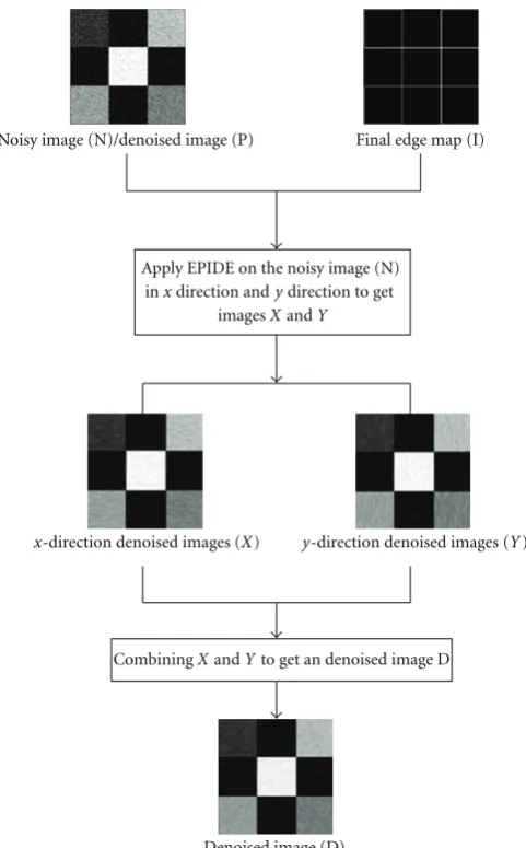
N o i s y i m a g e ( N ) / d e n o i s e d i m a g e ( P ) F i n a l e d g e m a p ( I )
D e n o i s e d i m a g e ( D ) imagesXandY
CombiningXandYto get an denoised image D
x-direction denoised images (X) y-direction denoised images (Y) Apply EPIDE on the noisy image (N)
inxdirection andydirection to get
Figure6: The flow chart to get denoised image at the final stage.
Equation (15) can easily be solved to obtainbn:
bn(t)=
exp
−n2π2t L2
t
0βn·
exp
n2π2s
L2
ds. (16)
Then solutionu(x,t) is obtained by substituting this formula forbninto (13).
2.3. Proposed Procedure. The goal of the proposed procedure with four stages is to preserve the desired edges during the image processing of noise reduction, so EPIDE method plays an important role. However, the edges of object contours in an image should be extracted previously for EPIDE method. Canny edge detector can automatically find some edges in images. Since the contour edges are not all found, then the users want to interactively modify the edges capture all desired object contours.
In the first stage of the procedure, any kind of denoising algorithm can be applied on an original noisy image to obtain a denoised image. In the second stage, an edge map can be obtained to find the edges of the object contours by
the Canny edge detector applied on the previously denoised image at the first stage. Since the contour edges are not found completely, then the users may be need to interactively modify the edge map to keep the edges of the desired object contours. At the third stage, users can manually modify the edges of edge map to match the desired edges. At the final stage, Edge Preserved Inhomogeneous Diffusion Equation (EPIDE) method is used to smooth the original noisy image or the previously denoised image at the first stage and achieve preserving desired edge. Two flow charts of the proposed procedure are shown in Figures5and6.
(a)
(b) (c)
(d) (e)
(f) (g)
Figure7: Comparing the performance of the various noises on “Nine Square Regions”. (a) Original Image. (b) Gaussian noise image,
(a) (b)
(c) (d)
(e)
Figure8: (a) “Nine Square Regions”, (b) noisy image with Gaussian noise withσ =0.01, (c) wavelet, PSNR=25.493, (d) ADF, PSNR=
23.835, and (e) the proposed procedure, PSNR=28.495.
At the final stage, the EPIDE method is used to smooth the noisy image (N) or the previously denoised image (P) with the modified edge map (I). Both inx-direction and y -direction, two imagesXandY are generated by the EPIDE method. Finally a denoised image (D) can be obtained by an average combination of the imageXandY.
3. Experimental Results
There are four test images “Nine Square Regions”, “Number and Character”, “Chinese Words”, and “BarCode” corrupted by Gaussian noise with zero mean.
3.1. The Peak Signal-to-Noise Ratio (PSNR). The perfor-mance measure by using the peak signal-to-noise ratio is defined as follows:
PSNR=20·log10 255
RMSE, (17)
where RMSE is Root Mean Square Error, and it is defined as follows:
RMSE=
1
m×n m
i=1
n
j=1
fi,j−gi,j2. (18)
The functions f(i,j) andg(i,j) are original and denoised image, respectively. The numbersmandnare the size of an image.
(a)
(b)
(c)
(d)
(e)
Figure 9: (a) “Number and Character”, (b) noisy image with Gaussian noise withσ=0.01, (c) wavelet, PSNR=21.946, (d) ADF, PSNR=22.285, and (e) the proposed procedure, PSNR=22.495.
3.2.1. Noise Reduction Test. The experiments tested the synthetic image “Nine Square Regions” with Gaussian noise, Salt-and-Pepper noise, and Poisson noise, the result are shown inFigure 7.
The test image “Nine Square Regions” is a synthetic image shown in Figure 7(a). Figure 7(b) is the test image corrupted by adding Gaussian noise with variance 0.01. Figure 7(d)is the test image corrupted by adding salt and pepper noise with the density 0.05. Figure 7(f) is the test image corrupted by adding Poisson noise. Figures7(c),7(e), and 7(g) are images denoised by proposed procedure to preserve edges.
3.2.2. Comparison with Algorithms. In the experiments we have used the geometric images “Nine Square Regions”, “Number and Character”, “Chinese Words”, and “BarCode” in order to demonstrate the edge preservation capability of the proposed procedure. Corresponding to three denoising methods, the values PSNR of all the denoised images are given inTable 1. These results of PSNR are 28.495, 22.495, 20.769, and 28.021 for four test images “Nine Square Regions”, “Number and Character”, “Chinese Words” and
(a)
(b)
(c)
(d)
(e)
Figure10: (a) Four Chinese words, (b) noisy image with Gaussian noise withσ=0.05, (c) denoised image by wavelet, PSNR=16.453, (d) denoised image by ADF, PSNR=17.244, and (e) the proposed procedure, PSNR=20.769.
“BarCode” by the proposed procedure. The PSNR values of the proposed procedure are larger than those of the wavelet and ADF denoising method. The proposed procedure has better denoising capability.
The test image “Nine Square Regions” is a synthetic image shown in Figure 8(a). Figure 8(b) is the test image corrupted by adding Gaussian noise with variance 0.01. Figure 8(c) is the denoised image by wavelet denoising method.Figure 8(d)is the denoised image by ADF denoising method.Figure 8(e)is the denoised image by the proposed procedure. From the visual evaluation of images (c), (d), and (e), the proposed procedure has the best edge preservation.
(a) (b)
(c) (d)
(e)
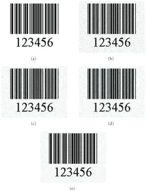
Figure11: (a) BarCode image, (b) noisy image with Gaussian noise withσ =0.05, (c) denoised image by wavelet, PSNR =17.762, (d) denoised image by ADF, PSNR=16.940, and (e) denoised image by the proposed procedure, PSNR=28.021.
Table1: RMSE and PSNR (dB) values of the denoised images by EPIDE, Wavelet, and ADF methods. There are four test images “Nine Square Regions”, “Number and Character”, “Chinese Words”, and “BarCode”.
Image Nine Square Regions Number and Character Chinese Words BarCode
RMSE PSNR RMSE PSNR RMSE PSNR RMSE PSNR
Noise Image 21.809 21.358 23.885 20.568 40.206 16.045 18.197 22.931 EPIDE 9.5896 28.495 19.133 22.495 23.340 20.769 10.127 28.021 Wavelet 13.549 25.493 20.379 21.947 38.319 16.453 32.994 17.762 ADF 16.397 23.835 19.602 22.285 35.022 17.244 36.27 16.940
is the denoised image by the proposed procedure. From the visual evaluation of images (c), (d), and (e), the proposed procedure has the best edge preservation.
The test image “Chinese Words” is an image with four Chinese characters as shown in Figure 10(a). Figure 10(b) is the test image corrupted by adding Gaussian noise with a variance of 0.05. Figure 10(c) is the denoised image by wavelet denoising method. Figure 10(d) is the denoised image by ADF denoising method. Figure 10(e)is the denoised image by the proposed procedure. From the visual evaluation of images (c), (d), and (e), the proposed procedure has the best edge preservation.
The test image “BarCode” is an image without noise as shown in Figure 11(a). Figure 11(b) is the test image corrupted by adding Gaussian noise with variance 0.05.
Figure 11(c) is the denoised image by wavelet denoising method.Figure 11(d)is the denoised image by ADF denois-ing method. Figure 11(e) is the denoised image by the proposed procedure. From the visual evaluationof images (c), (d), and (e), the proposed procedure has the best edge preservation.
(a) (b)
(c) (d)
(e) (f)
(g) (h) (i)
(a) (b)
(c) (d)
(e) (f)
(g) (h)
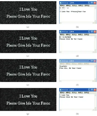
Figure13: Left column is (a) noisy image and denoised image by (c) wavelet (e) ADF and (g) the proposed procedure, right column. (b), (d), (f), and (h) are OCR results.
edge detector and the results of denoised image by EPIDE method.Figure 12(a)is a synthetic image andFigure 12(b) is the noisy image with Gaussian noise with σ = 0.05. Figure 12(c)is an edge map obtained by Canny edge detector applied onFigure 12(b).Figure 12(d)is the denoised image by EPIDE method applied on Figure 12(b) with the edge map in Figure 12(c). Figure 12(e) is a denoised image by neighborhood filters applied on Figures 12(b)and12(f)is an edge map by Canny edge detector applied onFigure 12(e). Figure 12(g)is a manually modified edge from the edge map ofFigure 12(f).Figure 12(h)is the denoised image by EPIDE method with the edge map inFigure 12(g)applied on image in Figure 12(e), but Figure 12(i) is the denoised image by EPIDE method with the same edge map applied on image in Figure 12(b). By the visual evaluations,Figure 12(i)is better thanFigure 12(h). FromTable 2, the PSNR values of image ofFigure 12(i)is higher thanFigure 12(h). The first stage of proposed procedure can be an option for different images denoising cases.
Table2: RMSE and PSNR (dB) values of denoised images B, D, H and I.
B D H I
RMSE 6.3711 3.7040 3.6321 3.1651 PSNR 32.049 36.757 36.928 38.123
∗
Character “B” representsFigure 12(b). ∗Character “D” representsFigure 12(d). ∗Character “H“ representsFigure 12(h). ∗Character “I” representsFigure 12(i).
0 50 100 150 200 0
50 100 150 200 250
(a)
0 20 40 60 80 100 120 140 160 180 200 0
50 100 150 200 250
(b)
0 50 100 150 200
0 50 100 150 200 250 300
(c)
0 50 100 150 200
0 50 100 150 200 250 300
(d)
0 50 100 150 200
0 50 100 150 200 250
(e)
0 50 100 150 200
0 50 100 150 200 250
(f)
Figure14: The 20th row ofu(x,y) of the image “Nine Square Regions” with the various noise. (a) Gaussian noise, (c) Salt and Pepper noise, (e) Poisson noise. The denoised results are, respectively, (b), (d), and (f)
and it’s variance is 0.08. The denoised images are shown in Figures13(c),13(e)and13(g)and they are denoised by wavelet, ADF and EPIDE methods. Figures 13(b), 13(d), 13(f)and13(h)are OCR results of images in the left column. To evaluate the denoising performance of wavelet, ADF and EPIDE methods, it is suitable to use the character recognition software JOCR [16] to obtain the words in noised and denoised images. The experimental results show that the image denoised by EPIDE can have the best recognition
results in Figure 13(h). All the characters in two sentences “I Love You“ and “Please Give Me Your Favor” are correctly recognized in the image denoised by EPIDE method. There are some errors for character recognition are in Figures 13(b),13(d)and13(f). These results are obtained by JOCR software on the noisy and denoised images by wavelet and ADF methods.
section, theoretical explanations are described to show why the proposed denoising procedure works well for any kind of noise.
3.2.5. The Denoising Capability of the Diffusion Equation. There are many types of image noise, such as Gaussian noise, Salt-and-pepper noise, Shot noise and Uniform noise. Noises are randomly distributed in image intensity value. At different pixels, the intensity values are independent of one another. For example, Gaussian noise, Shot noise and Uniform noise separately follow a Gaussian, Poisson, Fat-tail and Uniform distribution. The 20th row of u(x,y) of the image “Nine Square Regions” inFigure 7with Gaussian noise, Salt and Pepper noise and Poisson noise has three profiles as in Figures 14(a), 14(c), and 14(e). The three profiles of the denoised image are shown in Figures14(b), 14(d), and14(f). Three profiles as in Figures14(a),14(c), and 14(e)are the initial conditions of the diffusion equation (6). Three profiles as in Figures 14(b),14(d), and14(f)are the steady-state solutions of the steady-state diffusion equation (19)
K∇2u(x,t) +F(x)=0. (19)
The image denoising results in Figures 14(b), 14(d), and 14(f)are consistent with the theoretical explanation of (19).
4. Conclusion
The contribution of the paper is to propose a procedure to smooth the noisy or denoised image with any kind of denoising algorithm for desired edge preservation. To achieve preservation of designed edges, the inhomogeneous terms of the diffusion equation are formulated by the derivative of the Delta function. Fourier series is used to obtain the exact solution of the diffusion equation. The exact solution is a function of time and its value is the intensity of each pixel in an image. The Delta functions in the diffusion equation are used to locate the positions of edge pixels for each object in the image. To locate contour pixels for each object, it is necessary to use some image preprocessing methods and an edge detection method to find the edges of the object contours. Since the contour edges are not all found, then the user can interactively modify the edge map to keep the desired object contours. The proposed denoising method with edge preservation capability has the best OCR result in the experiment compared to the results from the wavelet denoising method and anisotropic diffusion filters.
Acknowledgment
The authors thank National Science Council (NSC) for partial financial support (NSC 97-2115-M-324-001) and (NSC 98-2115-M-324-001).
References
[1] W. E. Weideman, M. T. Manry, and H. C. Yau, “A comparison of nearest neighbor classifier and a neural network for
numeric handprint character recognition,” in Proceedings of the IEEE International Conference on Neural Networks, Washington, DC, USA, 1989.
[2] C. C. Tappert, “Recognition System for Run-on Handwritten Characters,” US patent no. 4731857, International Business Machines Corporation, Armonk, NY, USA, March 1988. [3] S.-H. Hahn, J.-H. Lee, and J.-H. Kim, “A study on utilizing
OCR technology in building text database,” in Proceedings of the 10th International Workshop on Database and Expert Systems Applications, pp. 582–586, 1999.
[4] R. C. Gonzalez and R. E. Woods, Digital Image Processing, Prentice-Hall, Upper Saddle River, NJ, USA, 2002.
[5] M. Welk and J. Weickert, “Semidiscrete and discrete well-posedness of shock filtering,” in Mathematical Morphology, Springer, Berlin, Germany, 2005.
[6] S. Guillon, P. Baylou, M. Najim, and N. Keskes, “Adaptive nonlinear filters for 2D and 3D image enhancement,”Signal Processing, vol. 67, no. 3, pp. 237–254, 1998.
[7] Y. B. Yuan, T. V. Vorburger, J. F. Song II, and T. B. Renegar, “A simplified realization for the Gaussian filter in surface metrology,” inProceedings of the 10th International Colloquium on Surfaces, M. Dietzsch and H. Trumpold, Eds., p. 133, Shaker, Chemnitz, Germany, January-February 2000. [8] P. Perona and J. Malik, “Scale-space and edge detection using
anisotropic diffusion,”IEEE Transactions on Pattern Analysis and Machine Intelligence, vol. 12, no. 7, pp. 629–639, 1990. [9] S. K. Weeratunga and C. Kamath, “A comparison of
PDE-based non-linear anisotropic diffusion techniques for image denoising,” in Image Processing: Algorithms and Systems II, Proceedings of SPIE, Santa Clara, Calif, USA, January 2003. [10] G. Gerig, O. Kubler, R. Kikinis, and F. A. Jolesz, “Nonlinear
anisotropic filtering of MRI data,” IEEE Transactions on Medical Imaging, vol. 11, no. 2, pp. 221–232, 1992.
[11] R. P. Kanwal,Generalized Functions: Theory and Applications, Birkh¨auser, Boston, Mass, USA, 3rd edition, 2004.
[12] G. B. Folland, Fourier Analysis and Its Applications, Brooks/Cole, Pacific Grove, Calif, USA, 1992.
[13] M. Sen,Analytical Heat Transfer, Department of Aerospace and Mechanical, Engineering University of Notre Dame, Notre Dame, Ind, USA, 2008.
[14] R. Bracewell, The Fourier Transform and Its Applications, McGraw-Hill, New York, NY, USA, 2nd edition, 1986. [15] J. Canny, “A computational approach to edge detection,”IEEE
Transactions on Pattern Analysis and Machine Intelligence, vol. 8, no. 6, pp. 679–698, 1986.