Multichannel SAR Interferometry via Classical
and Bayesian Estimation Techniques
Alessandra Budillon
Dipartimento per le Tecnologie, Universit`a degli Studi di Napoli “Parthenope,” via Acton 38, 80133 Napoli, Italy Email:[email protected]
Giancarlo Ferraiuolo
Dipartimento di Ingegneria Elettronica e delle Telecomunicazioni, Universit`a degli Studi di Napoli “Federico II,” via Claudio 21, 80125 Napoli, Italy
Email:[email protected]
Vito Pascazio
Dipartimento per le Tecnologie, Universit`a di Napoli “Parthenope,” via Acton 38, 80133 Napoli, Italy Email:[email protected]
Gilda Schirinzi
Dipartimento di Automazione Elettromagnetismo Ingegneria dell’Informazione Matematica Industriale (DAEIMI), Universit`a degli Studi di Cassino, via Di Biasio 43, 03043 Cassino, Italy
Email:[email protected]
Received 10 August 2004; Revised 20 January 2005
Some multichannel synthetic aperture radar interferometric configurations are analyzed. Both across-track and along-track in-terferometric systems, allowing to recover the height profile of the ground or the moving target radial velocities, respectively, are considered. The joint use of multichannel configurations, which can be either multifrequency or multi-baseline, and of classical or Bayesian statistical estimation techniques allows to obtain very accurate solutions and to overcome the limitations due to the presence of ambiguous solutions, intrinsic in the single-channel configurations. The improved performance of the multichannel-based methods with respect to the corresponding single-channel ones has been tested with numerical experiments on simulated data.
Keywords and phrases:synthetic aperture radar interferometry, statistical signal processing, Markov random fields.
1. INTRODUCTION
Synthetic aperture radar interferometric (InSAR) systems use more than one antenna (typically two), which can be dis-placed along the platform moving direction (along-track in-terferometry) or along the direction orthogonal to the mov-ing direction (across-track interferometry). From the acqui-sitions of two or more image signals, these systems are able to recover additional information about the observed scene: they allow the reconstruction of the height profile of the earth surface in the across-track configuration [1, 2], and the detection of moving targets on the ground and the es-timation of their range velocity in the along-track config-uration [3, 4]. This is possible because the interferomet-ric phase, that is, the (−π,π] wrapped phase of the sig-nal obtained from the point-to-point correlation between the complex images acquired from the two interferometric
antennas, is related the height values of the ground (for the across-track interferometry) and to the range velocity (for the along-track interferometry), through a known mapping. Then, after the so-calledphase unwrapping(PhU) operation, a map of the ground elevation, for the first case, or of the target range velocity, for the latter case, can be retrieved.
solution ambiguities are present. Moreover, they do not take into account the statistical properties of the noise present on the data (i.e., not Gaussian [2]). Other interferometric tech-niques using multipass acquisitions have been proposed in literature [8,9,10].
In the along-track InSAR system, the problem is quite similar, but in this case only very few (typically only one) pix-els of the image, the ones corresponding to the moving tar-get, are involved. From one side, this simplifies the estimation procedure, from the other, it does not allow to introduce con-textual information between adjacent pixel for increasing the estimation accuracy, like it happens in the across-track case. Moreover, other parameters besides coherence, such as the signal to clutter ratios, have to be considered. In the case of high signal-to-clutter ratio, the velocity can be easily recov-ered inverting a simple algebraic relation. When the signal-to-clutter ratio decreases, the velocity estimation becomes gradually more and more critical, till it fails completely. Also in this case, as in the across-track case, there are solution am-biguities which can keep the velocity estimation from work-ing correctly [11].
We propose to solve both above-mentioned problems by using statistical estimation methods, and exploiting multi-channel interferograms. The statistical estimation methods allow to take into account from one hand the correct statistics of the involved noise (likelihood model); on the other hand, they can allow to model the same unknown of the problem as a random field (a priori statistical model). In such a way, it can be possible to design optimum estimation procedures. The use of a multichannel interferogram, which in this case can be obtained exploiting frequency diversity and/or base-line diversity, has a twofold effect: multichannel interfero-grams can help to reduce the variance of the estimation, and, if properly chosen, can allow to avoid solution ambiguities [12,13,14].
In particular, for the across-track case, we describe a Bayesian estimation method formulated in terms of maxi-mum a posteriori (MAP) estimation of the ground elevation profile. Asa prioristatistical description, capable of model-ing pixels contextual information of the 2D height profile, a Gaussian Markov random field (GMRF) [15,16] has been considered. This model is tuned and matched to the true height profiles thanks to the so-called hyperparameters [15] which can be estimated starting from the same measured wrapped phase data. In this situation, uniqueness is guar-anteed by the use of multifrequency data. To take into ac-count contextual information about the neighboring clusters and the use of multichannel interferograms allows the recon-struction of critical (for other PhU methods) profiles in the presence of nonnegligible noise.
As far as the along-track case is considered, a classi-cal estimation method formulated in terms of maximum-likelihood (ML) estimation is adopted for the range-velocity estimation. Also in this case, the use of a multichannel con-figuration allows to estimate range velocities that cannot be estimated (because ambiguous) according to single-channel-based algorithms.
h P R1
R2
Ground track 1 Ground
track 2
Antenna 1 Baseline
Antenna 2
Flight track 2 Flight track 1
Figure1: Across-track SAR interferometry geometry. An arbitrary pointP whose quota ishis viewed from the two interferometric antennas with two different distancesR1andR2, respectively.
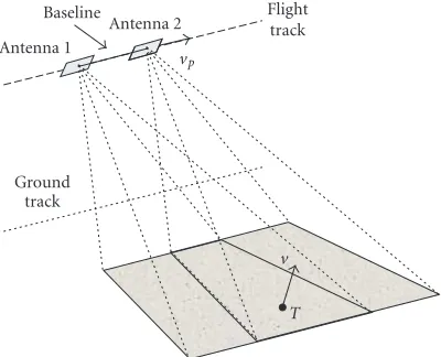
T v Ground
track Antenna 1
Baseline
Antenna 2 vp
Flight track
Figure 2: Along-track SAR interferometry geometry. A target T moving on the ground, whose velocity isv, is viewed with two dif-ferent phase histories from the two interferometric antennas mov-ing at velocityvp.
Some simulations and numerical experiments will also be presented to show and to validate the improved performance of multichannel-based methods with respect to single-channel ones.
2. SAR INTERFEROMETRIC SYSTEMS
Consider in more detail the two different SAR geometries adopted for the across-track interferometry (Figure 1) and along-track interferometry (Figure 2).
Assuming a discrete ground coordinate system (i,j),i=
z2(i,j) be thecomplexSAR image of the same ground region acquired by the second antenna.
The SAR interferometric signal is given by the complex correlation between the two SAR complex images:
y(i,j)=z1(i,j)z∗2(i,j), (1)
and the SAR interferometric phase signal is given by
φ(i,j)=tan−1Im
y(i,j)
Rey(i,j), (2)
where Re[·] and Im[·] represent the real and imaginary parts of a complex quantity.
The phase values obtained by (2) using actual data are noisy. In the across-track case, their nominal (noise-free) val-uesφ0(i,j) contain the information about the quota values [2]:
φ0(i,j)=
4πd λ h(i,j)
2π
, (3)
whereλis the wavelength corresponding to the working fre-quency f =c/λof the SAR system,dis a parameter related to the orthogonal component of the baseline of the interfer-ometric SAR system, and·2πrepresents the “modulo-2π”
operation.
In the along-track case, the interferometric phase nomi-nal valuesφv(i,j) contain the information aboutvr, the range
component of the object velocity (orthogonal and coplanar to the platform motion direction) [3]:
φv(i,j)=
4πb
λ
vr(i,j)
vp
2π =
4πb
λ ur(i,j)
2π
, (4)
where b is a quantity related to the parallel component of the baseline,vpis the velocity of the flying platform, and the
normalized range velocityurhas been introduced, where the
moving target is present,vr =0 and consequentlyφv(i,j)=
0, otherwise the along-track inteferometric phase (4) is null. The actual interferometric phase signalφ(i,j) (also called interferogram) differs from the nominal values given by (3) and (4) for the presence of phase noise. Also for the phase noise there are differences between the across-track and along-track cases which will be discussed in the follow-ing sections.
2.1. Across-track interferometric phase first-order probability density function
In the across-track case, the first-order probability density function (pdf) of the interferometric phaseΦis given by the well-know expression [17] (in the following we will use cap-ital letters to denote random variables):
fΦφ;φ0,γ
= 1
2π
1− |γ|2 1− |γ|2cos2φ−φ0
×
1 +|γ|cos
φ−φ0 cos−1− |γ|cosφ−φ0
1− |γ|2cos2φ−φ0 1/2
,
φ∈(−π,π], (5)
whereγis the coherence coefficient representing the corre-lation between images z1(·) andz2(·) at (i,j) andφ0is the nominal (noise-free) phase defined in (3). The local depen-dence ofφ,φ0, andγon (i,j) has been omitted to preserve the notation simplicity.
Some plots of pdf (5) forφ0 = 0 and for five different values ofγare shown inFigure 3. The larger the coherence value (its maximum is one) the more peaked the pdf. For different values ofφ0=0, the curve maximum is located on φ0.
To restore a better physical meaning, pdf (5) can be rewritten substituting (3) in (5), and exploiting the 2π -periodic nature of the cosine function:
fΦ(φ|h;λ,d,γ)= 1
2π
1− |γ|2
1− |γ|2cos2φ−(4πd/λ)h
1 +|γ|cos
φ−(4πd/λ)h cos−1− |γ|cosφ−(4πd/λ)h 1− |γ|2cos2φ−(4πd/λ)h
1/2 ,
φ∈(−π,π]. (6)
Equation (6) has been written as a conditional pdf, pointing out that the quotahcan be viewed in its turn as a random parameter.
Note that also for h = 0 (the case of a pure phase noise) the probability density corresponding to nonzero phase values is different from zero. This happens when the
−3 −2 −1 0 1 2 3 φ
0 0.2 0.4 0.6 0.8 1
fΦ
(
φ
)
γ=0.9 γ=0.7 γ=0.5 γ=0.3 γ=0.1
Figure 3: pdf of the interferometric phase forφ0 = 0 andγ =
0.1, 0.3, 0.5, 0.7, and 0.9.
It will be a useful result in the following sections, when the multichannel algorithm will be discussed.
2.2. Along-track interferometric phase first-order probability density function
Let Zc1 = Zc1r + jZc1i andZc2 = Zc2r + jZc2i be the
clut-ter processes representing the SAR complex images acquired from the two antennas in the along-track SAR interferometry case.
It is well known that the SAR image of most natural scenes is a (complex) random process, whose real and imag-inary parts are Gaussian, with zero mean and same variance, and uncorrelated [18], since they are resulting from the su-perposition of the signals backscattered from many scattering centers lying in the resolution cell. Then the joint probability density function ofZc=[Zc1r Zc1i Zc2r Zc2i]T is Gaussian,
that is,
fZc
zc = fZc1r,Zc1i,Zc2r,Zc2i
zc1r,zc1i,zc2r,zc2i
= 1
(2π)2Cc1/2exp
−1
2z
T cC−1c zc
, (7)
whereCcis the covariance matrix of real processesZc1r,Zc1i,
Zc2r, andZc2i,|Cc|is the determinant ofCc, andC−1c is the
inverse ofCc. The column vectorzcis defined as
zc=
zc1r zc1i zc2r zc2i. (8)
SinceZcis a zero-mean random vector, the covariance matrix
Ccis defined as
Cc=EZcZTc
=
VarZc1r E
Zc1rZc1i
EZc1rZc2r
EZc1rZc2i
EZc1iZc1r
VarZc1i E
Zc1iZc2r
EZc1iZc2i
EZc2rZc1r
EZc2rZc1i
VarZc2r E
Zc2rZc2i
EZc2iZc1r
EZc2iZc1i
EZc2iZc2r
VarZc2r
. (9)
Since Zc1 and Zc2 are the lowpass representations of nar-rowband signals it can be assumed that E[Zc1rZc1i] =
E[Zc2rZc2i] = 0, E[Zc1rZc2r] = E[Zc1iZc2i], E[Zc1iZc2r] = −E[Zc1rZc2i] (E[·] is the statistical average operator), and
Var(Zc1r)= Var(Zc1i)= Var(Zc2r) =Var(Zc1i)= σ2.
Con-sidering the coherence of the clutterγc(i.e., the complex
cor-relation coefficient ofZc1andZc2), defined as
γc= E
Zc1Zc∗2
VarZc1 VarZc2 1/2
= E
Zc1rZc2r
+jEZc1iZc2r
σ2 =
q σ2,
(10) we derive Cc=
σ2 0 Re(q) −Im(q) 0 σ2 Im(q) Re(q) Re(q) Im(q) σ2 0
−Im(q) Re(q) 0 σ2
. (11)
The presence of thermal noise at the receivers can be formalized considering two additive (to the clutter) zero-mean Gaussian complex processes N1 = N1r + jN1i and
N2 =N2r+ jN2i, independent of each other, and
indepen-dent of the clutter processes, with Var(N1r) = Var(N1i) =
Var(N2r)=Var(N2i)=σn2and covariance matrixCn=σn2I.
The two new processes representing the SAR images in pres-ence of thermal noiseZc1+N1andZc2+N2will have a co-variance matrix equal to
Cc+Cn=
σ2+σ2
n 0 Re(q) −Im(q)
0 σ2+σ2
n Im(q) Re(q)
Re(q) Im(q) σ2+σ2
n 0
−Im(q) Re(q) 0 σ2+σ2
n . (12)
The main effect of thermal noise amounts to reduce the co-herence, now given by
γ= E
Zc1+N1 Zc2+N2 ∗
VarZc1+N1 VarZc2+N2 ]1/2
=E
Zc1rZc2r
+jEZc1iZc2r
σ2+σ2
n
= q
σ21 +σ2
n/σ2
= γc
1 +σ2
n/σ2
.
(13)
Being the clutter and the noise processes stationary and zero mean, the termσ2
n/σ2represents the ratio between the power
of the thermal noise and the power of the clutter. Its inverse σ2/σ2
ncan be defined as the clutter-to-noise ratio (CNR).
−3 −2 −1 0 1 2 3 φ
0 0.2 0.4 0.6 0.8 1 1.2 1.4 1.6 1.8
fΦ
(
φ
)
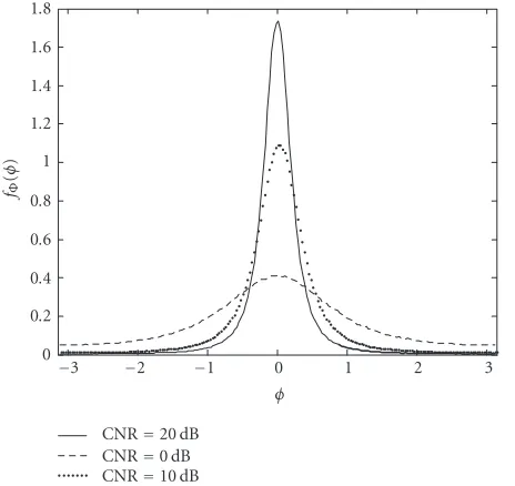
CNR=20 dB CNR=0 dB CNR=10 dB
Figure 4: pdf of the interferometric phase in absence of moving target (φv=0), for three values of CNR(0, 10, 20 dB), andγc=0.95.
In presence of a moving target, the SAR complex images become
Z1= Zc1
+N1+zT1 in presence of moving target, Zc1+N1 in absence of moving target
Z2= Zc2
+N2+zT2 in presence of moving target, Zc2+N2 in absence of moving target,
(14)
wherezT1andzT2denote the SAR (deterministic) images of the moving target relative to the two interferometric anten-nas (approximately 2D sinc signals in case of concentrated target).
The two processesZ1=Z1r+jZ1iandZ2=Z2r+jZ2iare
still Gaussian, have mean (due to the moving target) different from zero:
mZ=EZ1r Z1i Z2r Z2iT
=RezT1 Im
zT1 Re
zT2 Im
zT2 T, (15)
and same covariance matrix of the clutter-plus-noise process given byCz =Cc+Cn. The interferometric signal is finally given by the productZ1Z2∗=Aexp(jΦ).
The adopted model provides in absence of moving tar-gets the pdf of the interferometric phase shown inFigure 4. Note that this pdf can also be obtained analytically from (5) settingγ=γc/(1 + 1/CNR), as shown in (13).
In presence of moving targets, the interferometric phase pdf depends on the CNR, on the coherenceγc, on the
signal-to-clutter ratio (SCR), defined as the ratio between the inten-sity of the moving target and the power of the background clutter in the resolution cell, and also on the target range
−3 −2 −1 0 1 2 3
φ 0
0.5 1 1.5 2 2.5
fΦ
(
φ
)
SCR=20 dB SCR=0 dB SCR=10 dB
Figure5: pdf of the interferometric phase in presence of a moving target such thatφv =2.0 rad, for three values of SCR(0, 10, 20 dB),
CNR=10 dB, andγc=0.95.
velocity through (4). Note that in along-track InSAR applica-tions, the coherence is close to one. The statistical description of the interferometric phaseΦcan be derived numerically via Monte Carlo techniques.
The pdfs of the interferometric phase evaluated for a range velocity such that the nominal value isφv = 2.0 rad,
for three values of SCR(0, 10, 20 dB), for CNR =10 dB, and a clutter coherenceγc=0.95, are shown inFigure 5.
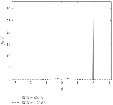
Despite the lack of availability of an analytical form of this interferometric phase pdf, it is possible to make rea-sonings under the hypothesis of high and low SCRs. In the first case, the signal components zT1 andzT2 prevail over to clutter-plus-noise components. Consequently, Z1 ≈ zT1 and Z2 ≈ zT2 andZ1Z∗2 = zT1zT∗2 = A2Texp(jφv), where
A2
T is the moving target power. The overall random phase
Φ of the interferometric signal tends toward the determin-istic constantφv, and its pdf tends toward a Dirac delta (see
Figure 6). On the other hand, in the case of low SCR values, the clutter-plus-noise components prevail against the signal components, the interferometric signal tends toward the one relative to the absence of a moving target, and the phase pdf can be obtained as inFigure 4setting the proper value ofγc
and CNR. A numerical confirmation of the above discussion is shown inFigure 6, where the pdfs relative to SCR=60 dB (high) and SCR= −20 dB (low) are reported.
It has to be noted that the probability density function of the interferometric phase in presence of moving targets (see Figure 5) is not given by the shift, of a quantity equal toφv, of the pdf in absence of moving target (seeFigure 4),
as sometimes reported in literature. For the pdfs reported inFigure 5, only the one relative to SCR = 20 dB (CNR =
10 dB,γc = 0.95) is centered onφv, but its values are very
−3 −2 −1 0 1 2 3 φ
0 5 10 15 20 25 30
fΦ
(
φ
)
SCR=60 dB SCR= −20 dB
Figure6: pdf of the interferometric phase in presence of a moving target such thatφv =2.0 rad, CNR=10 dB,γc =0.95, and for a
high value of SCR (60 dB) and a low value of SCR(−20 dB).
to the same values of CNR andγcinFigure 4. For lower
val-ues of SCR, neither a shift equal toφvnor the preservation of
pdf values is guaranteed, as shown in Figures5and6, and this circumstance must be taken into proper account if one wants to correctly detect moving targets and retrieve their velocities in along-track InSAR applications.
3. MULTICHANNEL ACROSS-TRACK SAR
INTERFEROMETRY: HEIGHT RECONSTRUCTION Across-track SAR interferometric (InSAR) systems allow the reconstruction of the height profile of the earth surface [1]. It consists of the transformation of themodulo-2π(wrapped) interferometric phase signal into a (unwrapped) phase signal whose values are not limited to the interval (−π,π]. As this unwrapped phase signal is related to the height profile of the earth surface [1,2], this operation allows recovering the ter-rain topographic map. It should be noted that the unwrap-ping problem is ill-posed, since it admits an infinite number of solutions [12,13].
Recently, two methods for overcoming this limitation, restoring the solution uniqueness by exploiting different data sets acquired with frequency diversity, have been proposed [12,13,14]. The unknown terrain profile is reconstructed from the knowledge of multiple wrapped interferometric phase (statistically independent) signals obtained with differ-ent working frequencies of the SAR system. They are based on maximum likelihood (ML) estimation techniques, and the multifrequency interferograms are obtained by subband filtering interferometric images [12,13] splitting the overall bandwidth as shown inFigure 7. The multiple interferogram needed to reconstruct the height profile can be obtained also starting from a multi-baseline system configuration [8] (see Figure 8). We will refer in the following to multifrequency
and/or multi-baseline configuration as multichannel config-uration.
The first technique [12, 13] is based on classical esti-mation techniques, in particular, on maximum likelihood (ML) estimation, and can be implemented in a strictly lo-cal way [12] or by exploiting deterministic contextual infor-mation consisting in the approxiinfor-mation of the height surface through local planes [13]. The extension of the strictly lo-cal technique [12] to take into account deterministic contex-tual information [13] allows better reconstructions also in the presence of nonnegligible noise and by using reduced-bandwidth systems [13].
The second technique [14] is based on Bayesian esti-mation techniques, in particular, on maximum a posteriori (MAP) estimation. Its implementation allows to overcome some limitations of ML multichannel approaches, and allows to reduce the number of interferograms with respect to the above-mentioned ML algorithms to obtain reliable height es-timation. In the following, we describe in more detail the Bayesian technique.
3.1. Multichannel maximum a posteriori estimation of height profiles
Consider a discrete (lexicographically ordered) two-dimensional (2D) point lattice L = {k, k =1,. . .,M×P}
on the ground, and let h = [h1 h2 · · · hM×P]T be the
corresponding ground elevation values. Consider now an InSAR (interferometric synthetic aperture radar) system and letφknbe the wrapped phase value measured at the lattice
pointkand at the working frequencyνn = c/λn, wherecis
the speed of the light (we assume here that the ground scene is observed withNdifferent sensors working atN different frequencies). The wrapped phase values φkn relative to the
position kand frequencyνncan be structured and ordered
in the following way: letΦk =[φk1 φk2 · · · φkN]T be the
vector of the wrapped phases measured atkat theN differ-ent working frequencies, let Φ = [ΦT1 Φ2T · · · ΦTM×P]T
be the vector collecting all available wrapped phase values (multifrequency interferograms), and let hbe the vector of the unknown height values. The multi-baseline case can be easily derived by the following development by varyingdin place ofλ.
Considering the statistical description of the phase noise samples, the mapping between phase values and height val-ues, and the hypothesis of statistical independence between the phase noise samples, the likelihood function of the height values, once all values of wrapped phase have been measured, turns out to be [14]
Fm f(Φ|h)= M×P
k=1
N
n=1
fΦφkn|hk;λn,d,γkn , (16)
whereγknis the coherence coefficient at positionkand
fre-quencyνn =c/λn, and fΦ(·) is given by (6) consideringhk
as unknown once thatφkn has been measured. We refer to
ν1 ν2 ν3 ν4 . . . ν5 ν6 ν7 ν8 Range frequency
BI BII
Bd
Azimuth frequency
L1 L2 L3 L4
1 2 3 4
5 6
16
17 18
21
32
Figure7: Partition of the dual band spectrum of a hypothetical SAR interferometric system. The two bandsBIandBIIare subband filtered
intoNr =8 range subbands (central frequenciesν1,ν2,. . .,ν8), and the Doppler bandBdintoNa =4 azimuth looks (L1,L2,L3,L4). Each
(n=1,. . .,N =Na×Nr =32) identifies a portion of the 2D frequency domain not overlapping with the others. Absence of overlapping
guarantees the statistical independence of interferograms [13].
Antenna 1 Baseline 1
Antenna 2
Baseline 2 Antenna 3
Figure8: Multi-baseline (in particular, dual-baseline) across-track SAR interferometric system.
In terms of the MAP approach, the unknown image is a random vectorHwith an assigneda prioristatistical distri-bution. In our case, being the unknown image representative of the elevation of a geographic area, a strong contextual pixel information is very likely to be. In particular, we assume that the unknown image can be modeled as aMarkov random field (MRF) [15], a general image model able to represent contex-tual pixel information extending the 1D Markov property to the 2D case. In particular, we choose a Gaussian Markov ran-dom field (GMRF) [16] as model, whose expression, say it gH, is
gH(h;σ)= 1
Z(σ)exp
−E(h;σ)
= 1
Z(σ)exp −
M×P
k=1
j∈Nk
hk−hj 2
2σk j2
,
(17)
where Z(σ) = ∫exp{−E(h;σ)}dh is the so-called parti-tion funcparti-tion [16], E(·) is the energy function, σ is the
hyperparameter vector [16], Nk is the neighbourhood
sys-tem ofkth pixel [15] (usually, the 8 pixels around thekth one), andσk jare the singlehyperparameters. ThelocalGMRF
model in (17) well adapts to describe the image local na-ture, by tuning the hyperparameters, leading to a powerful and general model, well suited to represent a wide class of height profiles.
These hyperparameter values have to be estimated from the same interferograms, through an ML estimation. This es-timation problem is not trivial, and requires the adoption of approximations, as the use of the MPL (maximum pseudo-likelihood) [19] to overcome the problems related to the use of the multivariate partition functionZ(σ) [15]. Finally, the expectation-maximization(EM) algorithm [16] allows to for-mulate the expression of the hyperparameter estimation up-date at (i+ 1)th iteration:
σ2
k(i+ 1)=E
"
j∈Nk
hk−hj 2
9 |Φ,σk(i) ,
σ2
k(i+ 1) −→ ilargeσ#
2
k,
(18)
where the expected value is evaluated on random variableHk
and the factor 9 in the denominator is resulting from the average over the chosen neighbourhood, formed by 9 pix-els. For its evaluation, thanks to ergodicity of the a posteriori distribution [15], we can approximate this expected value by “time” averaging, sampling from the a posteriori distribu-tion, which is itself an MRF, so that a Gibbs sampler [15] can be used for generating its samples. In particular, we use a Metropolis[19] version of this algorithm.
Once that the hyperparameter vector has been estimated, say itσ, the MAP estimation can be formulated as#
#
hMAP=argmax
h
fPost(h|Φ)
=argmax
h
lnFm f(Φ|h)gH(h;σ#),
where fPost(h|Φ) is thea posteriorijoint pdf of the unknown image, and the “hat” denotes the estimated values. Then, the solution procedure essentially consists of two steps: (i) ML estimation (σ) of the hyperparameter vector# σ; (ii) MAP esti-mation (#hMAP) of the actual realization of height profile pro-cessH.
For the MAP estimation, we use thesimulated anneal-ing (SA) [19] algorithm. In order to avoid excessive time-consuming a semideterministic approach, which guarantees a reliable convergence, is adopted. Since the knowledge of the hyperparametermap is effective to avoid local minima in the image formation process, we follow this strategy: after hyper-parameter estimation, we initialize the reconstruction algo-rithm with a high probability image sample, generated dur-ing the parameter estimation step, and startdur-ing from it we get the solution by ICM (iterated conditional modes) algorithm [19], which is deterministic, and then very fast.
4. MULTICHANNEL ALONG-TRACK SAR INTERFEROMETRY RANGE-VELOCITY ESTIMATION
Along-track synthetic aperture radar interferometry (AT-InSAR) is a technique used to detect moving objects (ocean surface [3], ships, vehicles on ground [20]) by means of two (or more) SAR antennas mounted on the same platform flying along a linear trajectory at constant velocity vp , as shown inFigure 2, and to recover their range velocities. As already shown in by (4), the noise-free nominal interfero-metric phase is related to the range (orthogonal and coplanar to the platform motion direction) component of the object velocity.
The moving object detection capability and the accuracy of the velocity estimation depend essentially on the target range velocity and on three parameters: SCR, CNR, and clut-ter coherenceγc. For detecting the moving targets in the SAR
images, a possible strategy amounts to compare the interfero-metric phase with a threshold. Of course, at different choices of the threshold correspond different false-alarm probabil-ity (PFA) and detection probability (PD). For estimating the
target range velocity, in AT-InSAR applications, only one or very few pixels can be exploited, differently from the across-track case, where contextual relations between neighbour-ing pixels help to reconstruct the height profiles. In case of low SCR, a single value of the interferometric phase, which is noisy and characterized by a polarized pdf (see pdf in Figure 5), does not guarantee faithful detection and estima-tion.
In the following section, we show how the use of a multi-channel, which also in this case can be multifrequency and/or multi-baseline, will help to find a reliable solution to this problem. As far as the multifrequency configuration is con-sidered, the choice of the different frequencies is the same adopted in the across-track case (seeFigure 7). As far as the multi-baseline configuration is concerned, the multiple an-tennas have to be positioned along the flight trajectory as shown inFigure 9.
T v
Ground track
Ground Baseline 2
Antenna 1
Antenna 2 Baseline 1 Antenna 3
vp
Flight track
Figure9: Multi-baseline (in particular, dual-baseline) along-track SAR interferometric system.
The method adopted for the velocity estimation is based on an ML approach and exploit multichannel interferomet-ric phase.
4.1. AT-InSAR moving target detection capabilities
Consider a point target moving with constant velocityv =
uxvpx+urvpr, whereuxandur, with|ux|,|ur| 1, are the
dimensionless target velocity components along the x (az-imuth) andr(slant range) coordinates, scaled to the platform velocityvp= |vp|.
As shown inSection 2, the range velocity affects the inter-ferometric phase which in the ideal noise-free case is given by the deterministic quantityφv = (4πb/λ)ur2π, while in the
real case becomes a random variableΦdistributed according a pdf depending on several parameters:
fΦφ|ur;λ,b,γc, SCR, CNR . (20)
Of course, in absence of a moving target (ur=0, and SCR=
0) (20) reduces to (5) withφ0 = 0, and is available in ana-lytical form. It has to be noted that both pdfs (20) and (5) are defined in the interval (−π,π] highlighting the wrapped nature of the available actual interferometric phase.
A moving target can be detected by comparing the in-terferometric phaseφwith a thresholdφT, and this threshold
has to be fixed in the interval (−π,π]. Starting from the avail-able pdfs relative to the hypotesis of presence and absence of moving target, we can evaluate the detection and false-alarm probability in the following way:
PD=
$−φT
−π fΦ
φ|ur;λ,b,γc, SCR, CNR dφ
+ $π
φT fΦ
φ|ur;λ,b,γc, SCR, CNR dφ,
PFA=2
$π
φT fΦ
φ|0;λ,b,γc, 0, CNR dφ.
The plot of some pdfs relative to a given value of velocity such thatφv=2 (rad), toγc=0.95, to SCR=0, 10, 20 (dB),
and CNR =0, 10, 20 (dB), and the relativePD are shown in
Figure 10.
The detection probability appears more sensitive to SCR than to CNR values. For values of SCR = 10 and 20 dB, PD ≈1 for threshold values lower than 1, for SCR =0 [dB]
(the powers reflected from the moving target and the clutter are equal in the resolution cell), a threshold lower than 0.5 still guaranteesPD≈1.
The plot of the pdf relative to absence of moving target obtained forγc = 0.95, and CNR = 0, 10, 20 (dB), and the
relativePFAare shown inFigure 11.
If one wants to keep low values ofPFA, for instance, equal
toPFA=0.1, a threshold equal to 0.6, 0.9, and 2.2 (rad) must
be used for the cases relative to CNR = 20, 10, and 0 (dB), respectively. In correspondence of these values,PD ≈ 1 for
SCR =20 (dB),PD ≥0.95 for SCR=10 (dB), andPD
col-lapses toward values 0.1/0.2 for SCR=0 (dB).
The performance of the detection process is, as expected, better for high values of SCR, that is, when the moving tar-gets power is significantly larger than the clutter power. For moving targets mingling with the background clutter, the de-tection capability worsens, so that if one wants low values of PFA, thePD can decrease to very low values, not consistent
with the applications.
It has to be considered that such performance is obtained starting from a single interferometric phase value. Exploit-ing multichannel information and a proper processExploit-ing of the available data phase vector, such performance can be signifi-cantly improved.
4.2. AT-InSAR moving target range-velocity estimation
The next step after the detection of the moving target is the estimation of its normalized range velocity ur. It has to be
remembered that phase values outside interval (−π,π) wrap mod(2π), so that such values are indistinguishable from the ones differing for 2π multiples, and the same holds for the corresponding velocity values. It results that the maximum range-velocity value that can be unambiguously detected is given by
±π=4πb
λ ur,max=⇒ur,max= λ
4b. (22)
We propose a new method for recover the range velocity, whose values can be ambiguous, based on the use of a mul-tichannel along-track SAR interferometer exploiting an ML approach.
Following the same approach outlined in [12,13], the SAR complex images can be subband filtered at different cen-tral frequencies in order to generate samples of the inter-ferometric phase at different wavelengthλn(n = 1,. . .,N),
and/or a multi-baseline configuration can be adopted, ob-taining different baseline bm (m = 1,. . .,M). Main
ef-fect of the use of multichannel interferograms is the veloc-ity ambiguveloc-ity suppression. In fact, at different wavelength and/or at different baseline, as it can be inferred by (22), the
ambiguous velocity changes. Properly combining this “mul-tichannel” phase information relative to different frequencies and/or different baselines, it can be highlighted [12] that the maximum likelihood (ML) estimation of the target velocity is not ambiguous.
This approach is based on the construction of the mul-tichannel likelihood function that can be obtained by multi-plying the likelihood functions corresponding to the central frequency of the subbands and to the different baselines:
Lur =
n,m
fΦφn,m|ur;λn,bm,γc, SCR, CNR , (23)
where φn,m represents the wrapped phase values relative to
the frequencyc/λn, and to the baselinebm. The factorization
(23) comes from the statistical independence of the multi-channel interferograms.
The ML estimation of the range velocity from the multi-channel data is finally given by
#
ur=argmax
ur L
ur . (24)
5. NUMERICAL RESULTS
5.1. Multichannel MAP-MRF height reconstructions
We test the performance of the MRF-MAP method pre-sented inSection 3.1for a simulated height profile, consid-ering the DEM of the Isolation Peak(Colorado), shown in Figure 12a. The used interferograms presented in Figures12b and 12c are, respectively, simulated at Nr=2 different fre-quencies (ν1 =5 GHz andν2 =9 GHz), and the coherence value isγ=0.85 for both frequencies.
For each working frequency,Na=4 looks are generated
by bandpass filtering of the azimuth spectrum, so allowing to generateN=Nr×Na=8 independent interferograms. The
adopted system parameters, including the coherence value, are those of the SRTM mission [21].
−3 −2 −1 0 1 2 3 φ
0 0.5 1 1.5 2 2.5
fΦ
(
φ
)
SCR=20 dB SCR=0 dB SCR=10 dB
(a)
0 0.5 1 1.5 2 2.5 3 φT
0 0.1 0.2 0.3 0.4 0.5 0.6 0.7 0.8 0.9 1
PD
SCR=20 dB SCR=0 dB SCR=10 dB
(b)
−3 −2 −1 0 1 2 3
φ 0
0.5 1 1.5 2 2.5
fΦ
(
φ
)
SCR=20 dB SCR=0 dB SCR=10 dB
(c)
0 0.5 1 1.5 2 2.5 3 φT
0 0.1 0.2 0.3 0.4 0.5 0.6 0.7 0.8 0.9 1
PD
SCR=20 dB SCR=0 dB SCR=10 dB
(d)
−3 −2 −1 0 1 2 3
φ 0
0.5 1 1.5 2 2.5
fΦ
(
φ
)
SCR=20 dB SCR=0 dB SCR=10 dB
(e)
0 0.5 1 1.5 2 2.5 3 φT
0 0.1 0.2 0.3 0.4 0.5 0.6 0.7 0.8 0.9 1
PD
SCR=20 dB SCR=0 dB SCR=10 dB
(f)
Figure10: (a), (c), and (d) pdfs relative to a given value of velocity such thatφv =2 (rad), toγc =0.95, to SCR =0, 10, 20 (dB), and
−3 −2 −1 0 1 2 3 φ
0 0.2 0.4 0.6 0.8 1 1.2 1.4 1.6 1.8
fΦ
(
φ
)
CNR=20 dB CNR=0 dB CNR=10 dB
(a)
0 0.5 1 1.5 2 2.5 3
φT
0 0.1 0.2 0.3 0.4 0.5 0.6 0.7 0.8 0.9 1
PFA
CNR=20 dB CNR=0 dB CNR=10 dB
(b)
Figure11: (a) pdfs relative to absence of moving target forγc=0.95, CNR=0, 10, 20 (dB), and (b) relative false-alarm probabilities.
5.2. Multichannel ML range-velocity estimation
We present some results relative to the application of the multichannel-based method to a hypothetical airborne sys-tem. The chosen central working frequency is 5.3 (GHz) (the corresponding wavelength is λc = 0.0566 (m)), and the
ve-locity of the platform is fixed tovp=200 (m/s). We consider
and discuss three system configurations:
(a) total bandwidthB = 100 (MHz), single baselineb =
0.25 (m);
(b) total bandwidthB = 400 (MHz), single baselineb =
0.25 (m);
(c) total bandwidthB = 50 (MHz), dual baselineb1 =
0.25 (m),b2=0.42 (m).
In case (a), the maximum unambiguous range velocity is given by|ur,max| = λ/4b = 0.056. In terms of absolute ve-locity, this value corresponds to|vr,max| = |ur,max| ×vp =
11.32 (m/s) = 40.75 (km/h). Such result means that by us-ing a sus-ingle-channel along-track interferometer (one base-line, one frequency), it is not possible to infer the velocity of a target moving with a range velocity larger than|ur,max|, even if the key parameters assume very favourable values (e.g., large values of SCR andγc, and low values of CNR).
A target with a large radar cross-section as a car or a truck (σT ≥ 100 (m2), then providing a large SCR) moving at a
range velocity about equal to±2|ur,max| = ±81.5 (km/h) is seen as still clutter (such value of velocity wraps on a nomi-nal interferometric phase equal to 0).
For this reason, we subband partition the available system bandwidth intoNa=8 looks andNr=4 range subbands, so
allowing to generate N = Nr×Na = 32 independent
in-terferograms. Such interferograms are not characterized by
very different central frequencies so a strong capacity is not expected to avoid the velocity ambiguity [13]. To run the numerical experiments, we fix the following values: γc =
0.95 (typical values for AT-InSAR application are larger than 0.95), SCR=10 (dB) (usually for airborne applications SCR values are larger, but in this case, we considered the effect of multilooking), and CNR=20 [dB] (such value can be much larger in airborne applications). The range velocity to be esti-mated has been chosenur=0.08, external to the
unambigu-ous interval. Such case cannot be treated with conventional single-baseline AT-InSAR. The results of the estimation are summarized in the first row ofTable 1, where in the left col-umn is reported the percentage of faithful estimation (errors lower than 3%), and in the right case the percentage of totally erroneous estimation. It has to be noted that the estimation method is potentially very accurate (the variance of the noise is not very high for such value of SCR, CNR, andγc), so that
the erroneous results are due to the estimation of ambigu-ous values: when the method works well, estimate is very accurate and close to the right solution; when the method does not work, estimate is very accurate and close to an am-biguous value of velocity. For this reason, a column reporting medium quality estimation is absent in the table.
The range velocity is correctly estimated in about the 50% of the considered cases, denoting the usefulness of the introduction of multichannel information. The percentage of correct estimation would have been 0% in a single-channel configuration.
Consider now case (b), where a larger bandwidth is avail-able for the subband partition. We filter outNa = 8 looks
andNr = 4 range subbands, so allowing to generateN =
Nr×Na=32 independent interferograms. The chosen range
0 100 200 300 400 500 600 700 800 900 1000
(a)
−3
−2
−1 0 1 2 3
(b)
−3
−2
−1 0 1 2 3
(c)
0 10 20 30 40 50 60 70 80 90 100
(d)
0 10 20 30 40 50 60 70 80 90 100
(e)
0 100 200 300 400 500 600 700 800 900 1000
(f)
Figure12: (a) Reference profile, (b) noisy (γ=0.85) interferogram at 5 Ghz (C band), (c) noisy (γ=0.85) interferogram at 9 Ghz (X band), (d) reference hyperparameter map, (e) hyperparameter map estimation from noisy interferograms, and (f) MAP reconstruction.
Table1: Range-velocity estimation performance. SCR=10 (dB), CNR = 20 (dB),γc = 0.95. Velocity to be estimatedur = 0.08,
out of the unambiguous interval (±0.056) of the InSAR system at fc =5.3 (GHz), andb =0.25 (m). Case (a) total bandwidthB =
100 (MHz), single baselineb=0.25 (m). Case (b) total bandwidth B=400 (MHz), single baselineb=0.25 (m). Case (c) total band-widthB=50 (MHz), dual baselineb1=0.25 (m),b2=0.42 (m).
Case Correct estimation (%) Wrong estimation (%)
Case (a) 50% 50%
Case (b) 68% 32 %
Case (c) 100% 0%
(a). The estimation results are reported in the second row ofTable 1. The range velocity is correctly estimated in about 68% of the considered cases, denoting the improved capac-ity deals with a set of central frequencies more different from each other than in case (a).
Finally, case (c) relative to a dual baseline configuration is considered. In this case, the available bandwidth has been reduced to 50 MHz, and a third antenna has been added in order to consider a dual-baseline (M =2) system. In order to generate the multichannel interferogram, for each base-line, we filter out Na = 8 looks andNr = 2 range
sub-bands, so allowing to generate N = Nr ×Na = 16
multi-frequency independent interferograms.M×N =32 chan-nels are available also in this case. The chosen range veloc-ity to be estimated isur =0.08, as in the previous cases (a)
and (b). In this case there are two values for the unambigu-ous range velocity, given by|u(r1,max) | = λ/4b1 = 0.056, and
the impressive capacity of a dual baseline system to estimate range velocity without incurring in ambiguous values of ve-locity.
One of the main consequences of an incorrect range-velocity estimation is a significant displacement of the mov-ing target in the SAR image. The estimated target velocities then can be exploited to relocate the moving objects in the right positions of the final SAR images.
6. CONCLUSIONS
Some techniques based on statistical estimation dealing with multichannel InSAR applications have been analyzed in this paper. It has been shown that the joint use of multichannel configurations and statistical solution techniques allows to widen the classes of height profiles and moving target ve-locity that can be reliably reconstructed. In particular, as far as the across-track case and the height profiles reconstruc-tion are concerned, the proposed MAP approach incorporat-ing the a priori statistical information of the height profiles through an MRF model has evidenced that it is not necessary to have at one’s disposal a large number of channels to get re-liable solutions. The same comments hold for the along-track case and the range-velocity estimation. The number of chan-nels necessary to reach good performances is sufficiently low, thus allowing the practical application of the method.
Multichannel data, which can be obtained by wideband systems and/or by more interferometric pairs of SAR images of the same ground area, are necessary to avoid solution am-biguities and to improve estimation accuracy. For this reason, the performance analysis results of multichannel configura-tions are very important for future interferometric missions planning.
REFERENCES
[1] S. N. Madsen, H. A. Zebker, and J. Martin, “Topographic mapping using radar interferometry: processing techniques,” IEEE Trans. Geosci. Remote Sensing, vol. 31, no. 1, pp. 246–256, 1993.
[2] R. Bamler and P. Hartl, “Synthetic aperture radar interferom-etry,”Inverse Problems, vol. 14, no. 4, pp. R1–R54, 1998. [3] R. M. Goldstein and H. A. Zebker, “Interferometric radar
measurements of ocean surface currents,”Nature, vol. 328, no. 6132, pp. 707–709, 1987.
[4] R. E. Carande, “Dual baseline and frequency along-track in-terferometry,” inProc. IEEE International Geoscience and Re-mote Sensing Symposium (IGARSS ’92), vol. 2, pp. 1585–1588, Houston, Tex, USA, May 1992.
[5] D. C. Ghiglia and M. D. Pritt,Two-Dimensional Phase Un-wrapping: Theory, Algorithms, and Software, John Wiley & Sons, New York, NY, USA, 1998.
[6] D. C. Ghiglia and L. A. Romero, “Robust two-dimensional weighted and unweighted phase unwrapping that uses fast transforms and iterative methods,”Journal of the Optical Soci-ety of America A, vol. 11, no. 1, pp. 107–117, 1994.
[7] M. Costantini, “A novel phase unwrapping method based on network programming,”IEEE Trans. Geosci. Remote Sensing, vol. 36, no. 3, pp. 813–821, 1998.
[8] A. Ferretti, C. Prati, and F. Rocca, “Multibaseline phase un-wrapping for InSAR topography estimation,” Il Nuovo Ci-mento, vol. 24, no. 1, pp. 159–176, 2001.
[9] J. Homer, I. D. Longstaff, Z. She, and D. Gray, “High res-olution 3-D imaging via multi-pass SAR,”IEE Proceedings -Radar, Sonar and Navigation, vol. 149, no. 1, pp. 45–50, 2002. [10] D. Massonnet, H. Vadon, and M. Rossi, “Reduction of the need for phase unwrapping in radar interferometry,”IEEE Trans. Geosci. Remote Sensing, vol. 34, no. 2, pp. 489–497, 1996.
[11] A. Budillon, V. Pascazio, and G. Schirinzi, “Multi-channel along track interferometry,” inProc. IEEE International Geo-science and Remote Sensing Symposium (IGARSS ’04), vol. 4, pp. 2601–2603, Anchorage, Alaska, USA, September 2004. [12] V. Pascazio and G. Schirinzi, “Estimation of terrain elevation
by multifrequency interferometric wide band SAR data,”IEEE Signal Processing Lett., vol. 8, no. 1, pp. 7–9, 2001.
[13] V. Pascazio and G. Schirinzi, “Multifrequency InSAR height reconstruction through maximum likelihood estimation of local plane parameters,”IEEE Trans. Image Processing, vol. 11, no. 12, pp. 1478–1489, 2002.
[14] G. Ferraiuolo, V. Pascazio, and G. Schirinzi, “Maximum a pos-teriori estimation of height profiles in InSAR imaging,”IEEE Geoscience and Remote Sensing Letters, vol. 1, no. 2, pp. 66–70, 2004.
[15] S. Geman and D. Geman, “Stochastic relaxation, Gibbs’ dis-tributions, and Bayesian restoration of images,”IEEE Trans. Pattern Anal. Machine Intell., vol. 6, no. 6, pp. 721–741, 1984. [16] S. S. Saquib, C. A. Bouman, and K. Sauer, “ML parameter estimation for Markov random fields with applications to Bayesian tomography,”IEEE Trans. Image Processing, vol. 7, no. 7, pp. 1029–1044, 1998.
[17] D. Just and R. Bamler, “Phase statistics of interferograms with applications to synthetic aperature radar,”Applied Op-tics, vol. 33, no. 20, pp. 4361–4370, 1994.
[18] J. C. Curlander and R. N. McDonough,Synthetic Aperture Radar, Wiley Interscience, New York, NY, USA, 1991. [19] S. Z. Li,Markov Random Field Modeling in Image Analysis,
Springer, Berlin, 2001.
[20] H. Breit, M. Eineder, J. Holzner, H. Runge, and R. Bamler, “Traffic monitoring using SRTM along-track interferometry,” in Proc. IEEE International Geoscience and Remote Sensing Symposium (IGARSS ’03), vol. 2, pp. 1187–1189, Toulouse, France, July 2003.
[21] J. E. Hilland, F. V. Stuhr, A. Freeman, et al., “Future NASA spaceborne SAR missions,”IEEE Aerosp. Electron. Syst. Mag., vol. 13, no. 11, pp. 9–16, 1998.
Alessandra Budillon received the Laurea degree (summa cum laude) in 1996, and the Ph.D. degree in 1999, in electronic engi-neering from the University of Napoli “Fed-erico II,” Napoli, Italy. From 2001 to 2004, she was an Assistant Professor at the De-partment of Information Engineering, the Second University of Nap, Aversa, Italy, and in November 2004, she joined the Depart-ment for Technologies, the University of
Giancarlo Ferraiuolo received the Laurea degree (summa cum laude) in electronic engineering from the Second University of Naples, Italy, in 2000, and the P.h.D. de-gree from the University of Napoli “Fed-erico II,” in 2004. In 2003, he spent a period as a Visiting Researcher in the Department of Electrical Engineering, Stanford Univer-sity, Stanford, Calif. Since December 2004, he has been a researcher at the Department
of Electronic and Telecommunication Engineering, the University of Napoli “Federico II.” His main scientific interests are in the field of statistical image formation for computed tomography and SAR applications.
Vito Pascazio graduated (summa cum laude) in 1986 from the University of Bari, Italy, in electronic engineering, and in 1990, he received the Ph.D. degree in electronic engineering and computer science from the Universit`a di Napoli “Federico II,” Italy. In 1990 he was first at IRECE-CNR, Napoli, Italy, and then, he joined the Universit`a di Napoli “Parthenope,” Italy, where he is presently a Full Professor of
telecommuni-cations. In 1994–1995, he was a Visiting Scientist at the Labora-toire des Signaux et Systemes, Ecole Superieure d’Electricite, Gif sur Yvette, France, and in 1998–1999 at Universit´e de Nice Sophia-Antipolis, France. His main scientific interests include statistical signal processing, remote sensing, and image computing and pro-cessing, and he is the author of more than 90 technical papers on international journals and conference proceedings. Dr. Pascazio is a Member of IEEE.
Gilda Schirinzi graduated in electronic engineering in 1983 from the Univer-sity of Napoli “Federico II.” In the same year, she joined the Electronic Engineer-ing Department as a Research Fellow. From 1985 to 1986, she was at European Space Agency, ESTEC, the Netherlands. In 1988, she joined Istituto di Ricerca per l’Elettromagnetismo e i Componenti Elet-tronici (IRECE), CNR, in Naples. In 1992,