Volume 2006, Article ID 92849, Pages1–14 DOI 10.1155/ASP/2006/92849
Optimum Wordlength Search Using
Sensitivity Information
Kyungtae Han and Brian L. Evans
Embedded Signal Processing Laboratory, Wireless Networking and Communications Group, The University of Texas at Austin, Austin, TX 78712, USA
Received 2 October 2004; Revised 4 July 2005; Accepted 12 July 2005
Many digital signal processing algorithms are first developed in floating point and later converted into fixed point for digital hardware implementation. During this conversion, more than 50% of the design time may be spent for complex designs, and optimum wordlengths are searched by trading offhardware complexity for arithmetic precision at system outputs. We propose a fast algorithm for searching for an optimum wordlength. This algorithm uses sensitivity information of hardware complexity and system output error with respect to the signal wordlengths, while other approaches use only one of the two sensitivities. This paper presents various optimization methods, and compares sensitivity search methods. Wordlength design case studies for a wireless demodulator show that the proposed method can find an optimum solution in one fourth of the time that the local search method takes. In addition, the optimum wordlength searched by the proposed method yields 30% lower hardware implementation costs than the sequential search method in wireless demodulators. Case studies demonstrate the proposed method is robust for searching for the optimum wordlength in a nonconvex space.
Copyright © 2006 K. Han and B. L. Evans. This is an open access article distributed under the Creative Commons Attribution License, which permits unrestricted use, distribution, and reproduction in any medium, provided the original work is properly cited.
1. INTRODUCTION
Digital signal processing algorithms often rely on long wordlengths for high precision, whereas digital hardware im-plementations of these algorithms need short wordlengths to reduce total hardware costs. Determining the opti-mum wordlength can be time-consuming if assignments of wordlengths are performed by trial and error. In a complex system, 50% of the design time may be spent on wordlength determination [1].
Optimum wordlength choices can be made by solving equations when propagated quantized errors [2] are ex-pressed in an analytical form. However, an analytical form is difficult to obtain in complicated systems. Searching the entire space by simulation guarantees to find optimum wordlength. Computation time, however, increases expo-nentially as the number of wordlength variables increases. For these reasons, many simulation-based wordlength opti-mization methods have explored a subset of the entire space [3–7].
Choi and Burleson [3] showed how a general search-based wordlength optimization can produce optimal or near-optimal solutions for different objective-constraint for-mulations. Sung and Kum [4] proposed simulation-based
wordlength optimization for fixed-point digital signal pro-cessing systems. These search algorithms try to find the cost-optimal solution by using either “exhaustive” search or heuristics.
Han et al. [5] proposed search algorithms that can find the performance-optimal solution by using “sequential” or “preplanned” search. Those algorithms utilize the distortion sensitivity information with respect to the signal wordlengths at the system output such as propagated quantized error. Those algorithms assume that the hardware cost in each wordlength is the same. However, complicated digital sys-tems such as a digital transceiver possess different cost or complexity in digital blocks.
A new algorithm that considers different hardware costs is proposed in [7]. The new algorithm utilizes the measure of the distortion sensitivity as well as complexity sensitivity. The new algorithm speeds up the search time to find an op-timum wordlength by considering performance and cost as the objective function and the update direction.
Table1: Fixed-point conversion approaches for integer wordlength (IWL) and for fractional wordlength (FWL) determination.
Analytical approach Statistical approach
Range model for IWL Error model for FWL Range statistic for IWL Error statistic for FWL
Wadekar [8] Constantinides [9] Cmar [10] Cmar [10]
Stephenson [11] Shi [12] Kim [13] Kum [14]
Nayak [15] — — Shi [12]
Table2: Optimum wordlength search methods.
Cost sensitivity Error sensitivity Nonsensitivity
Local search [3] Sequential search [5] Exhaustive search [4]
Evolutive search [6] Max-1 search [16] Branch and bound [3]
— Preplanned search [5]
Complexity-and-distortion measure search—proposed
update search directions are generalized in Section 5. Case studies of the optimum wordlength design are presented in Section 6. In Section 7, simulation results are discussed. Section 8concludes the paper.
2. RELATED WORK
During the floating-point to fixed-point conversion process, fixed-point wordlengths composed of the integer wordlength (IWL) part and the fractional wordlength (FWL) part are de-termined by different approaches as shown inTable 1. Some published approaches for floating-point to fixed-point con-version use an analytic approach for range and error estima-tion [8,9,11,12,15], and others use a statistical approach [10, 12–14]. An analytic approach has a range and error model for integer wordlength and fractional wordlength de-sign. Some use a worst-case error model for range estimation [8,15], and some use forward and backward propagation for IWL design [11]. Still, others use an error model for FWL [9,12]. The advantages of analytic techniques are that they do not require simulation stimulus and can be faster. How-ever, they tend to produce more conservative wordlength re-sults.
A statistical approach has been used for IWL and FWL determination. Some use range monitoring for IWL esti-mation [10,13], and some use error monitoring for FWL [10,12,14]. The work in [12] also uses an error model that has coefficients obtained through simulation. The advantage of statistical techniques is that they do not require a range or error model. However, they often need long simulation time and tend to be less accurate in determining wordlengths.
After obtaining models or statistics of range and error by analytic or statistical approaches, respectively, search al-gorithms can find an optimum wordlength. Some published methods search optimum wordlength without sensitivity in-formation [3,4], and with sensitivity information [3,5,16] as shown inTable 2. “Exhaustive” search [4] and “branch-and-bound” procedure [3] can find an optimum wordlength without any sensitivity information. However, nonsensitiv-ity methods have an unrealistic search space as the number of wordlengths increases.
Some use sensitivity information to search an optimum wordlength. “Local” search [3] and “evolutive” search in [16] use cost sensitivity information. The advantage of cost sensi-tivity methods is that they can find an optimum wordlength in terms of cost. “Sequential” search and “preplanned” search in [5] and “Max-1” search in [16] use error sensitivity infor-mation. The advantage of employing error sensitivity is that they find the optimum wordlength in terms of error faster than the cost sensitivity method. However, both sensitivity methods do not always reach global optimum wordlength.
Cantin et al. provide a useful survey of search algorithms for wordlength determination. In this work, search algo-rithms are compared, and the “preplanned search” shows the smallest number of iterations to find a solution. However, the heuristic procedures do not necessarily capture the op-timum solution to the wordlength determination problem, due to nonconvexity in the constraint space [9]. Thus, the distance between a global optimum wordlength and a local optimum wordlength searched by algorithms is considered. The proposed method is robust to search a near optimum wordlength. This paper discusses the distance and robustness of the proposed algorithm inSection 7.
3. BACKGROUND
3.1. Fixed-point data format
When designers model at a high-level, floating-point num-bers are useful to model arithmetic operations. Floating-point numbers can handle a very large range of values and are easily scaled. In hardware, floating-point data types are typi-cally converted or built as fixed-point data types to reduce the amount of hardware needed to implement the functionality. To model the behavior of fixed-point arithmetic hardware, designers need bit-accurate fixed-point data types.
corresponds to the following equation:
WL=IWL + FWL. (1)
The wordlength must be greater than 0. Given IWL and FWL, fixed-point data represents a value in the rangeR, with the quantization stepΔas
−2IWL≤R <2IWL, for signed,
0≤R <2IWL, for unsigned , Δ=2−FWL.
(2)
IWL and FWL are determined to prevent unwanted over-flow and underover-flow. IWL can be determined by the following relation:
IWL≥log2R. (3)
Here,xis the smallest integer that is greater than or equal tox. The range,R, can be estimated by monitoring the max-imum and minmax-imum value or mean and standard derivation of a signal [13,18]. FWL can be determined by wordlength optimization or tradeoffs in the design parameters during fixed-point conversion.
3.2. Formulation of the optimum wordlength
The wordlength is an integer value, and a set ofnwordlengths in a system is defined to be a wordlength vector, that is, w ∈Insuch as{w
1,w2,. . .,wn}. We assume that the
objec-tive function f is defined by the sum of every wordlength implementation cost functioncas
f(w)= n
k=1
ckwk, (4)
where ck has a real value so that ck : I → R. The quan-tized performance functionpindicates propagated precision or quantized error and is constrained as follows:
p(w)≥Preq, (5)
where p has a real value so that p : I → R, andPreq is a
constant for a required performance. We also consider the lower bound wordlengthwand upper bound wordlengthw as constraints for each wordlength variable:
wk≤wk≤wk, ∀k=1,. . .,n. (6)
The complete wordlength optimization problem can then be stated as
min
w∈In f(w) subject top(w)≥Preq,w≤w≤w. (7) The goal of the wordlength optimization is hence to search for the optimizerw∗ that minimizes the objective function
f(w) in (7).
3.3. Finding the optimum wordlength
One of the algorithms for searching the “optimum” wordlength starts with an initial feasible solutionw(0) and
performs an update via
w(h+1)=w(h)+sξ(h). (8)
Here,his an iteration index,sis the integer step size, andξ is an integer update direction. A sound initial guess, a well-chosen step size, and a well-well-chosen update direction can re-duce the number of iterations to find optimum wordlengths. Optimum wordlengths can be found by solving equa-tions when the performance function p is expressed in an analytical form. If there is no analytical form to express the performance, then simulation-based search methods can be used to search for optimum wordlengths by measuring the performance function. Typical approaches involve assigning wordlength vectorw(0)to a lower bound, an upper bound, or
a vector between the lower and upper bound. Step size can be fixed or adapted. The update direction is adapted according to the search algorithms inSection 4.
During iteration, the stopping criteria are dependent on the search algorithm. The algorithm that starts from the lower bound stops when the performanceP reaches the re-quired performancePreq. The algorithm that starts from the
upper bound stops whenPfalls belowPreq. Other algorithms
stop when the performanceP or costcconverges within a neighborhood.
4. REVIEW OF SIMULATION-BASED SEARCH METHODS
Optimum wordlengths can be found by solving equations when the performance functionPis expressed in an analyti-cal form. If there is no analytianalyti-cal form to express the perfor-mance, then simulation-based search methods can be used to search for optimum wordlengths by measuring the per-formance at the system output.
4.1. Complete search
Complete search (CS) tests every possible combination of wordlengths between the lower bound and upper bound and measures the performance of each combination by simula-tion. Then optimum wordlengths can be selected from the simulations results.
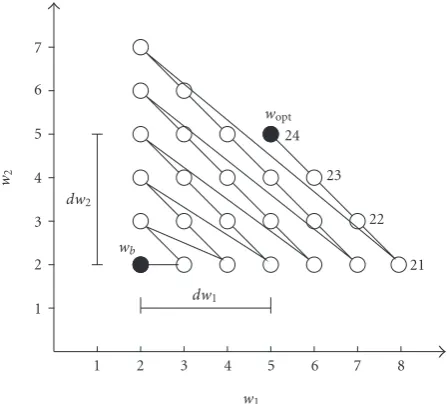
For example, assuming that the number of indepen-dent variables to find optimum wordlength is two, and the lower bound and upper bound are{2, 2}and{8, 7}, respec-tively, the possible wordlength combinations are shown in Figure 1. The number of trial tests or trials is 42. The opti-mum wordlength can be selected from the given simulation results after simulation completes.
The total number of tests inNwordlength variables is
EN
CS=
N
k=1
wk−wk+ 1
1 2 3 4 5 6 7 8 w1
1 2 3 4 5 6 7
w2
Figure1: The possible wordlength combinations searching the en-tire space in complete search (w= {2, 2};w= {8, 7}; trials =42).
1 2 3 4 5 6 7 8
w1
1 2 3 4 5 6 7
w2
dw1
dw2
wb
wopt
24 23
22 21
Figure2: The direction of exhaustive search (w= {2, 2}; optimum point= {5, 5}; distancedin (10) is 6; trials=24).
Complete search is guaranteed to find a global optimum point, but computational time and the number of tests increase exponentially as the number of wordlength variables increases.
4.2. Exhaustive search
Sung and Kum [4] search for the first feasible solution. They search for a wordlength with the minimum wordlength as the initial guess and increment the wordlength by one until the propagated error meets the minimum error. For example, assuming that we are trying to find the optimum wordlength for two variables, the minimum wordlengths are{2, 2}, and
each of wordlength cost is similar, the search path is shown in Figure 2. An optimized point{5, 5}is given for a comparison between search methods. The minimum number of trials is 24.
We have generalized the total number of experiments of the exhaustive search inN dimensions with the sum of the distance. The sum of the distance,d, is defined as
d=dw1+dw2+· · ·+dwN, (10)
wheredwiis the distance between the minimum wordlength and the optimum wordlength inith dimension. The expected number of experiments of the exhaustive search is calculated by using the summation of combination-with-replacement in [19] as
EN ES(d)=
d−1
r=0
CR(N,r)
=CR(N+ 1,d−1)=
N+d−1 d−1
= (N+d−1)!
(N+d−1)−(d−1)!(d−1)!
=(d+N−1)· · ·(d+ 2)(d+ 1)d
N! .
(11)
The trials may be bounded as
EESN(d)≤EN
,d
ES < ENES(d+ 1). (12)
The number of experiments is always less than that of com-plete search if at least two feasible solutions exist. However, the exhaustive search method is not always guaranteed in finding the global optimum.
4.3. Sequential search
The basic notion of sequential search is that each trial elimi-nates a portion of the region being searched [5]. This proce-dure is also called a “Min+b search” in [16]. The sequential search method decides where the most promising areas are located, and continues in the most favorable region after each set of experiments [20]. The sequential search algorithm can be summarized by the following four steps.
(1) Select a set of values for the independent variables, which satisfy the desired system performance during the one-variable simulations.
(2) Evaluate the system performance.
(3) Choose feasible locations at which system perfor-mance is evaluated.
(4) If the system performance of one point is better than others, then move to the better point, and repeat the search, until the point has been located within the desired accuracy. The base point is the minimum wordlength as an initial wordlengthw(0)in (8). In step (3), the direction of search,ξ
1 2 3 4 5 6 7 8 w1 1 2 3 4 5 6 7 w2 dw1 dw2 wb wopt
Figure3: The direction of sequential search (w= {2, 2}; optimum point= {5, 5}; distancedin (10) is 6; trials=12).
of their performance
ξj= ⎧ ⎪ ⎪ ⎪ ⎪ ⎪ ⎪ ⎪ ⎪ ⎪ ⎪ ⎨ ⎪ ⎪ ⎪ ⎪ ⎪ ⎪ ⎪ ⎪ ⎪ ⎪ ⎩
{1, 0, 0,. . ., 0}, ifmj= ∇ p w1,
{0, 1, 0,. . ., 0}, ifmj= ∇ p w2
,
· · ·
{0, 0, 1,. . ., 0}, ifmj= ∇ p wN,
mj=max
∇ p w1
,∇ p w2
,. . .,∇ p wN
,
(13)
where∇is the gradient operator.
InFigure 3, starting from wordlength base point{2, 2}, we measure performance of {2, 3} and {3, 2} from the direction of sequential search in step (3). If the performance of{3, 2}is better than that of{2, 3}, then a new wordlength vector moves into{3, 2}. Simulations are repeated until sat-isfying the desired performance.
We have generalized the trials of the sequential search in Ndimensions as
ENSS=N·
dw1+dw2+· · ·+dwN
. (14)
In this example, the numbers of trials are 12 from (14) and also 12 from Figure 3. The number of trials is re-duced by using sensitivity information. However, an opti-mum wordlength can be a local optima.
Local search [3] uses sensitivity information with the above procedure, but it uses cost sensitivity instead of per-formance sensitivity.
4.4. Preplanned search
A preplanned search [5] is one in which all the experi-ments are completely scheduled in advance. The directions
1 2 3 4 5 6 7 8
w1 1 2 3 4 5 6 7 w2 dw1 dw2 wb wopt
Figure4: The direction of preplanned search (w= {2, 2}; optimum point= {5, 5}; distancedin (10) is 6; trials=6).
are obtained from the sensitivity of performance of an inde-pendent variable. The optimum point is found by employing the steepest descent among local neighbor points.
The preplanned search algorithm in N dimensions is summarized by the following steps.
(1) Select a set of values for the independent vari-ables, which satisfy the desired performance during the one-variable simulations.
(2) Make a performance sensitivity list from the one-variable simulations.
(3) Make a test schedule with the sensitivity list to follow the higher sensitivity points from base point.
(4) Evaluate the performance at those points.
(5) Move to the points, until the point has been located within the desired accuracy.
In step (3), the direction of preplanned search is chosen in accordance with maximum derivative of an independent performance
ξj= ⎧ ⎪ ⎪ ⎪ ⎪ ⎪ ⎪ ⎪ ⎪ ⎪ ⎪ ⎨ ⎪ ⎪ ⎪ ⎪ ⎪ ⎪ ⎪ ⎪ ⎪ ⎪ ⎩
{1, 0, 0,. . ., 0}, ifmj= ∇p1 w1
,
{0, 1, 0,. . ., 0}, ifmj= ∇p2
w2
,
· · ·
{0, 0, 1,. . ., 0}, ifmj= ∇pN wN,
(15)
where
mj=max
∇p1 w1,∇
p2
w2
,. . .,∇pN wN
. (16)
RF demodulator
Carrier
LPF ADC Rake
receiver Decoder
Data output
(a) Analog demodulator.
RF demodulator
Carrier
ADC LPF Rake
receiver Decoder
Data output Output
SNR FER
(b) Digital demodulator.
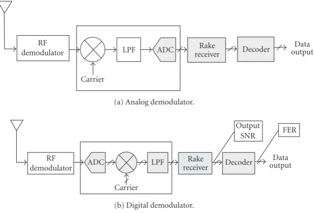
Figure5: Analog and digital demodulators in CDMA receiver and performance measurement position.
RF
Carrier
ADC LPF Rake
receiver Bi Bm
Bf c
Bf
Bc
Figure6: A digital demodulator block.
simulations atw1of 2 bits, is larger than that atw2for 2 bits,
then next feasible location is{3, 2}. Then, if the gradient at w1 of 3 is smaller than that atw2of 2, the next feasible
lo-cation is{3, 3}. The simulation path would be{2, 2},{3, 2}, {3, 3}, and so forth. After scheduling the feasible points, the performance of these points is evaluated until the value of the performance meets the desired accuracy.
We generalized the trials of the preplanned search inN dimensions as
EN
PS=dw1+dw2+· · ·+dwN. (17)
In this example, the trials are 6 from (17) and fromFigure 4. The number of trials is the least among the search meth-ods reported so far. However, finding the global optimum wordlength is not guaranteed.
4.5. Search example in CDMA demodulator wordlength design
Typical demodulators are implemented with an analog block in front of an analog-to-digital converter (ADC) block as shown in Figure 5(a). As the speed of the ADC increases, analog parts are replaced with digital parts in communica-tion systems [21]. We replaced the analog demodulator with the digital demodulator as shown inFigure 5(b).
The demodulator converts modulated signals into base-band signals. In the digital demodulator block ofFigure 6, the sampled data values output by the ADC are multiplied by a carrier signal to shift the spectrum down to the base-band. The out-of-band signal is removed by the lowpass fil-ter (LPF). The variables in the digital demodulator are given below [22,23]:
(i) (Bi): input wordlength; (ii) (Bc): carrier wordlength;
(iii) (Bm): multiplier output wordlength; (iv) (Bf): filter output wordlength;
(v) (Bf c): filter coefficient wordlength.
The output SNR is used for performance measurement instead of frame error rate (FER), which is a general surement to evaluate CDMA systems because direct mea-surement of FER requires at least 105frames during the
sim-ulation [24]. The required output SNR in this system is over 0.8 dB, or FER is under 0.03 [23].
Table3: Sequence of the sequential search for CDMA demodulator (traffic channel rate set 1 in additive white Gaussian noise, input
SNR= −17.3 dB,Eb/Nt=3.8, rate=9600 bps, and desired performance: output SNR>0.8 dB, FER<0.03).
Step {Bi,Bc,Bm,Bf,Bf c} Output SNR FER Result
1, 2 {4, 3, 4, 5, 7} 0.711 0.038 Fail
3 {5, 3, 4, 5, 7} 0.735 — —
3 {4, 4, 4, 5, 7} 0.694 — —
3 {4, 3, 5, 5, 7} 0.712 — —
3 {4, 3, 4, 6, 7} 0.759 — Max
3 {4, 3, 4, 5, 8} 0.704 — —
4 {4, 3, 4, 6, 7} 0.759 0.035 Fail
3 {5, 3, 4, 6, 7} 0.763 — —
3 {4, 4, 4, 6, 7} 0.722 — —
3 {4, 3, 5, 6, 7} 0.773 — Max
3 {4, 3, 4, 7, 7} 0.751 — —
3 {4, 3, 4, 6, 8} 0.749 — —
4 {4, 3, 5, 6, 7} 0.773 0.034 Fail
..
. ... ... ... ...
3 {6, 3, 5, 6, 7} 0.798 — —
3 {5, 4, 5, 6, 7} 0.802 — —
3 {5, 3, 6, 6, 7} 0.805 — Max
3 {5, 3, 5, 7, 7} 0.803 — —
3 {5, 3, 5, 6, 8} 0.798 — —
4 {5, 3, 6, 6, 7} 0.805 0.029 Pass
2 3 4 5 6 7 8 9 10
Wordlength 0.5
0.55 0.6 0.65 0.7 0.75 0.8 0.85 0.9 0.95 1
Output
SNR
Bi
Bc
Bm
Bf
Bf c
Figure7: Result of the independent one-variable simulations on a CDMA demodulator.
location because it has the largest communication perfor-mance. The simulation moves the current point to the new point and continues to search until the performance exceeds the specific desired requirement, which is an output SNR of 0.8 dB in this case. The final point is{5, 3, 6, 6, 7}, as shown inTable 3. The distance between the base and the optimum
point is 4 by using (10). The number of trials for the sequen-tial search to find an optimum wordlength is 20 by using (14).
In the preplanned search, the search path is esti-mated from the sensitivity of each one-variable simulation shown inFigure 7. Starting from the minimum wordlength or base point, {4, 3, 4, 5, 7}, the first expected point is {4, 3, 4, 6, 7} because Bf has the greatest derivative among each wordlength at the base point from Figure 7. The se-quence of the preplanned search points is {4, 3, 4, 5, 7}, {4, 3, 4, 6, 7},{4, 3, 4, 6, 8},{4, 3, 5, 6, 8},{4, 4, 5, 6, 8}, and so forth. Simulations move the current point to the next point until the performance exceeds the specific desired require-ment. The optimum point is{5, 4, 5, 6, 8}and distance is 5 by using (10). The number of trials of the preplanned search to find an optimum wordlength is 5 by using (17).
4.6. Comparison
Table4: Comparison of complete, exhaustive, sequential, and preplanned search (N =5,wk= {16, 16, 16, 16, 16},wk= {4, 3, 4, 5, 7}, and
the termdis defined in (10)).
Search Distance (d) Equation for number of experiments from (9), (11), (14), (17) Trials
Complete — Nk=1(wk−wk+ 1) 283920
Exhaustive 4 (d+ 4)(d+ 3)· · ·(d)/5! 56
Sequential 4 5·d 20
Preplanned 5 d 5
The exhaustive search needs 56 trials by using (11), which is less than the complete search. The exhaustive search is, however, inefficient to find the optimum wordlength when the wordlength variables for optimization are numerous and the distance between base and optimum point is longer.
The sequential search and preplanned search requires 20 and 5 trials, respectively, which are less than the other search methods. The preplanned search has the lowest number of experiments among search methods, but its distance using (10) is larger than that for sequential search. It implies that the wordlength of the sequential search method is closer to a global optimum with respect to hardware cost.
The sequential search and preplanned search have a loss of direction problem encountered by techniques based on the gradient projection method. This problem can be solved by adapting the step size.
The sequential search and the preplanned search reduce the trials by rates of 64% and 91%, respectively, when com-pared to the exhaustive search for wordlength optimization in the CDMA demodulator design. However, preplanned search seldom converges to the same optimum point, and the distance is longer than that of the other search methods.
5. SENSITIVITY MEASUREMENTS
The sensitivity information used for update directions in (8) can help reduce the search space dramatically. The sensi-tivity information can be obtained by measuring hardware complexity and distortion or propagated quantized precision loss. Complexity measure is used for hardware cost function in [3]. Distortion measure in [5] utilizes the sensitivity infor-mation of a propagated quantization error. Complexity-and-distortion measure in [7] combines two measures to update the search direction.
5.1. Complexity measure
The complexity measure method considers hardware com-plexity function as the cost function in (4) and uses the sensitivity information of the complexity as the direction to search for the optimum wordlengths. The local search in [3] uses complexity measure. The sensitivity information is cal-culated by gradient of the complexity function. For steepest descent direction, the update direction is
ξCM= −∇fc(w), (18)
where∇is gradient of function.
Complexity measure method updates wordlengths from the direction of the lowest sensitive complexity until a sys-tem meets a required performance such asPreq in (5). The
complexity measure method searches the wordlengths that minimize hardware complexity. However, it demands a large number of iterations since it does not use any distortion sen-sitivity information that can speed up to find the optimum wordlengths. For example, in a system composed of adders and multipliers, the complexity sensitivity of a multiplier is larger than that of an adder. The complexity measure method increases the wordlength in the adder with the right of pri-ority during an increase procedure even if the wordlength in the multiplier affects the propagated quantized performance more. It would waste computer simulation time if the com-plexity sensitivity of an adder is much smaller than that of a multiplier.
5.2. Distortion measure
The distortion measure method considers distortion func-tion as the objective funcfunc-tion in (4) and uses the sensitiv-ity information of the distortion for the direction to search for the optimum wordlengths. Sequential search uses distor-tion measure. This method assumes that every cost or com-plexity function would be the same or equal to 1, and selects wordlengths with the update direction according to the dis-tortion sensitivity information.
The complexity objective function is replaced with the distortion objective functiond(w) as
fd(w)=d(w), (19)
and the complexity minimization problem is changed into a distortion minimizing problem by
min
w∈In fd(w), subject tod(w)≤Dreq, c(w)≤Creq, w≤w≤w,
(20)
whereDreq is required distortion, andCreq is a complexity
constant.
The sensitivity information is also calculated by gradient of the distortion function. For the steepest descent direction, the update direction is
ξDM= −∇fd(w). (21)
For the distortion, Fiore and Lee [25] computed an error variance, and Han et al. [5] measured output SNR.
Data
source Encoder modulatorOFDM Channel
estimator
Decoder equalizerChannel BER
tester
Wireless channel model
OFDM demodulator
w0
w1
w2
w3
Figure8: Wordlength model for a fixed broadband wireless access demodulator.
the search direction depends on the distortion by chang-ing the wordlengths. This method rapidly finds the opti-mum wordlength satisfying the required performance by a fewer number of iterations compared to complexity measure method. However, the wordlengths do not guarantee the op-timum wordlengths in terms of the complexity.
5.3. Complexity-and-distortion measure
The complexity-and-distortion measure combines the com-plexity measure with the distortion measure by a weighting factor. In the objective function, both complexity and distor-tion are simultaneously considered. We normalize the com-plexity and the distortion function and multiply them with complexity and distortion weighting factors,αc andαd, re-spectively. The new objective function is
fcd(w)=αc·cn(w) +αd·dn(w), (22)
wherecn(w) anddn(w) are normalized complexity function and distortion function, respectively. The relation between the weighting factors is
αc+αd=1, (23)
where
0≤αc≤1, 0≤αd≤1. (24)
Using (22), the objective function gives a new optimiza-tion problem
min
w∈Infcd(w), subject tod(w)≤Dreq, c(w)≤Creq, w≤w≤w,
(25)
whereDreq andCreqare the required distortion and a
com-plexity constant, respectively. This optimization problem is to find wordlengths that minimize complexity and distortion simultaneously according to the weighting factors.
The update direction for the steepest decent direction to find the optimum wordlengthwis
ξCDM= −∇fcd(w). (26)
From (22) and (26), the update direction is
ξCDM= −
αc· ∇cn(w) +αd· ∇dn(w). (27)
Setting the complexity and distortion weighting factor, αcorαdfrom 0 to 1, the complexity-and-distortion method searches for an optimum wordlength with tradeoffs be-tween complexity measure method and distortion measure method. The complexity-and-distortion measure becomes the complexity measure or the distortion measure whenαd= 0 orαc=0, respectively.
The complexity-and-distortion measure method can re-duce the number of iterations for searching the optimum wordlengths, because the distortion sensitivity information is utilized. This method can more rapidly find the optimum wordlength that satisfies the required performance by using less iteration compared to the complexity measure method. However, the wordlengths are not guaranteed to be optimal in terms of the complexity.
6. CASE STUDY
6.1. OFDM demodulator design
Digital communication systems have digital blocks such as a demodulator that needs wordlength optimizations. Search-ing algorithms inSection 4were applied to the wordlength optimization of CDMA demodulator design inSection 4.5. From the CDMA case study, the sequential search is one of the promising methods to find an optimum wordlength. In this section, complexity measure, distortion measure, and complexity-and-distortion measure in Section 5 are applied in the sequential search framework to determine wordlengths for a fixed broadband wireless demodulator.
Fixed broadband wireless access technology is intended for high-speed voice, video, and data services, which is presently dominated by cable and digital subscriber line technologies [26]. One of the designs for orthogonal fre-quency division multiplexing (OFDM) demodulators for fixed broadband wireless access is shown inFigure 8. For the wireless channel, we used Stanford University Interim mod-els [27,28].
The main blocks in the demodulator for finite word-length determination are the fast fourier transform (FFT), equalizer, and estimator. For wordlength variables, we choose the wordlengths that have the most significant effect on com-plexity and distortion in the system. For the OFDM demod-ulator, we select wordlength variablesw0,w1,w2, andw3for
4 6 8 10 12 14 16 Wordlength
10−3
10−2
BER
w0
w1
w2
w3
Figure9: Wordlength effect for the demodulator inFigure 8, with Stanford University Interim wireless channel model number 3, SNR of 20 dB, FFT length of 256, and least-squares comb-type channel estimator without error-control coding.
We assume that the internal wordlengths of the given blocks have already been decided. In simulation, only the inputs to each block are constrained to be in fixed-point type, whereas the blocks themselves are simulated in floating-point type.
For the hardware complexity, the number of multipli-cations is measured assuming that processing units are not reused. The number of multiplications in a K-point FFT block is
CostFFT=K
2 log2K, (28)
where K is the number of taps. The cost of the 256-point FFT in the fixed broadband wireless access is estimated to be 1024. Approximately, the simplified complexity vectorc of the wordlength per bit is assumed to be{1024, 1, 128, 2} from [4,29].
We also assume the complexity increases linearly as wordlength increases to simplify demonstration. For the dis-tortion measurement, bit error rate (BER) is measured. The minimum wordlength searched by changing one wordlength variable, while other variables have high precision (i.e., 16 bits), is used for the initial wordlength [4,5]. The simulation for the minimum wordlength is shown inFigure 9.
Assuming the minimum performance of BER is 5×10⁻³,
the minimum wordlength is{5, 4, 4, 4}fromFigure 9. Start-ing from the minimum wordlength, wordlengths are in-creased according to the sensitivity information of diff er-ent measures inSection 5. We measure the number of iter-ations until they find their own optimum wordlength sat-isfying the required performance such as BER ≤ 2×10⁻³
without channel decoder. For the optimum wordlength, we follow the hybrid procedure [16] that combines a wordlength increase followed by a wordlength decrease. Simulation re-sults are presented inSection 7.
6.2. IIR filter case
OFDM demodulation case requires a large number of long simulations. This becomes especially time-consuming when each simulation takes hours in ensemble average of BER es-timation. For more general case, infinite impulse response (IIR) filter that has 7 wordlengths is simulated. There are various methods for getting error function and cost func-tion as described in related work secfunc-tion. For simplifying the simulation, mean square error (MSE) is measured for the error function, and a linear cost function of wordlength is assumed. Required performance of the IIR filter is assumed MSE of 0.1. In the IIR filter case study, the wordlength vector has 7 elements, and the hardware complexity of the arith-metic block has less difference when compared to the OFDM case study. Results are presented inSection 7.
7. RESULTS
The wordlength optimization problem is a discrete optimiza-tion problem with a nonconvex constraint space [30]. This nonconvexity makes it harder to search for a global optimum solution [31]. Tables5and6show that there are several lo-cal optimum wordlengths that satisfy error specification and minimize hardware complexity in case studies. In this sec-tion, wordlength optimization methods used in case studies are compared in terms of number of iteration and hardware complexity, and future work is discussed.
7.1. Number of iterations
The number of iteration to search an optimum wordlength in OFDM demodulator design is shown inFigure 10. The ini-tial wordlength does not satisfy the desired performance. Af-ter a number of trials by updating wordlength as in (8), the error at the system output decreases. The sequential search and the CDM search reach the feasible area after 15 trials. However, the local search takes 38 trials. After arriving at the feasible area, an optimum wordlength is searched again. In this case, the wordlengths, which are searched by the sequen-tial search or the CDM search, already arrive at an optimum wordlength. However, the local search needs more iterations to find an optimum wordlength. The total number of trials to find an optimum wordlength in each method for OFDM case is shown inTable 5. The sequential search and the CDM method can find an optimum solution in one-fourth of the time that the local search method takes.
Table5: Simulation results of several search methods starting from the minimum wordlength for the demodulator arcs inFigure 8.N=4,
wk= {5, 4, 4, 4}, andwk= {16, 16, 16, 16}. CDM is the complexity-and-distortion measure.αcis a weighting factor.
Search method αc Number of trials Wordlengths for variables Complexity estimate
Sequential search [5] 0 16 {10, 9, 4, 10} 10781
CDM 0.5 15 {7, 10, 4, 6} 7702
Local search [3] 1 69 {7, 7, 4, 6} 7699
Table6: Simulation results in IIR filter of several search methods.N=7,wk= {1, 1, 1, 1, 1, 1, 1}, andwk= {16, 16, 16, 16, 16, 16, 16}. CDM
is the complexity-and-distortion measure.αcis a weighting factor. (Max-1 search starts fromwk. Sequential search starts fromwk).
Search method αc Number of trials Wordlengths for variables Complexity estimate
Max-1 search [16] 0 94 {4, 5, 4, 5, 2, 2, 4} 378
Sequential search [5] 0 56 {4, 5, 4, 5, 2, 2, 4} 378
CDM 0.25 44 {4, 5, 4, 4, 2, 2, 5} 366
CDM 0.5 33 {6, 5, 5, 4, 1, 2, 4} 363
CDM 0.75 71 {6, 4, 4, 4, 2, 16, 13} 561
Local search [3] 1 126 {9, 5, 16, 4, 1, 16, 16} 723
5 10 15 20 25 30 35
Number of trials 10−3
10−2
BER
Sequential search CDM search (αc=0.5)
Local search
Figure10: Number of iterations for optimum wordlength with var-ious search algorithms in OFDM demodulator wordlength design.
search and the local search need a total of 56 and 126 itera-tions, respectively, including iterations in feasible and infea-sible area as shown inTable 6. The “Max-1” search starting from the feasible area needs 96 iterations. The CDM meth-ods with weighting factor of 0.25, 0.5, and 0.75 are used for comparison. When αc is less than 0.5, the CDM meth-ods have the property of the sequential search. Whenαc is greater than 0.5, the CDM methods search as the local search does. InFigure 11, the CDM methods with weighting factor of 0.25 and 0.75 show similar shape as the sequential search and the local search, respectively. In the IIR filter case, the CDM method withαcof 0.5 can find an optimum solution in one-fourth of the time that the local search method takes.
20 40 60 80 100 120
Number of trials 10−1
100
101
MSE
Sequential search αc=0.25
αc=0.5
αc=0.75
Local search
Figure11: Number of iterations for optimum wordlength in IIR filter with various search algorithms.
In general, if error sensitivity information for searching an optimum wordlength is used, the number of iterations can be reduced. The sequential search and the CDM method with less thanαc of 1 use the error sensitivity information. Thus, they converge quickly into an optimum wordlength that satisfies the required error performance.
7.2. Hardware complexity
Table7: Simulation results in noise cancellation with Wiener filter [32] of several search methods.N =5,wk = {1, 1, 1, 1, 1}, andwk = {16, 16, 16, 16, 16}. CDM is the complexity-and-distortion measure.αcis a weighting factor.
Search method αc Number of trials Wordlengths for variables Complexity estimate
Sequential search [5] 0 21 {4, 5, 5, 3, 2} 1331
CDM 0.25 23 {4, 4, 5, 4, 2} 1200
CDM 0.5 24 {5, 4, 4, 5, 4} 1074
CDM 0.75 167 {4, 4, 4, 5, 4} 1073
Local search [3] 1 170 {5, 4, 4, 15, 3} 1082
finds an optimum wordlength that has higher complexity than the CDM method and the local search in the OFDM demodulation case study. However, an optimum wordlength searched by the local search method, which uses hardware complexity information, has higher complexity in the IIR filter case study. If the design space is convex and has only one optimum solution, then various search methods find the optimum solution. However, wordlength optimization prob-lem has many local optimum solutions because of noncon-vex space. As the number of wordlength variables increases and as the system becomes more complicated, the probabil-ity in being stuck in a local optimum solution increases. In the IIR filter case with 7 elements in wordlength vector, the wordlengths searched by the local search method are far from globally optimal.
The CDM search with the weighting factor of 0.5 finds an optimum wordlength that has the lowest hardware complex-ity in this IIR case study. The CDM search with the weighting factor of 0.75 tends to be the local search. The hardware com-plexity from the CDM method of 0.75 is between the CDM of 0.5 and the local search. Similarly, the complexity from CDM method of 0.25 is between the sequential search and the CDM of 0.5.
For more examples, additional optimum wordlength search results in a noise cancellation with Wiener filter [32] are shown inTable 7.
7.3. Discussion
The CDM method, which uses error and complexity sensitiv-ity for optimum wordlength search, takes advantages from the sequential search and the local search. This method re-duces the number of iterations because of the error sensi-tivity that helps to fast reach feasible boundary. At the same time, this method finds a near-optimum wordlength that has lower hardware complexity because of the sensitivity of hardware complexity. The proposed method is robust for search optimum wordlength in a nonconvex space because this method is not easily captured by local optimum solu-tions.
The complexity-and-distortion measure method has flexibility to search for an optimum wordlength by setting weighting factor. Designer can select the weighting factor, αc, as in (23). Theαc of 0.5 means that the CDM method equally uses the sensitivity information of the error and the complexity. Theαcof 0.5 in CDM is reasonable for optimum wordlength search algorithms.
7.4. Future work
For an extension of work, various methods can be combined for wordlength optimization. Wordlength grouping [4] can be used to reduce a wordlength vector. Error model or error monitoring instead of error measuring can be used to reduce the simulation time. Actual cost model [12] can be used to get accurate result. For the searching method, different search methods such as binary search can be combined. Preplanned search, which is the fastest error sensitivity search method as compared in [16], can employ CDM methods to reach more quickly a near-optimum wordlength.
8. CONCLUSION
This paper generalized wordlength optimization methods that use sensitivity measures. The proposed complexity-and-distortion measure equation can express the local search or sequential search by changing the weighting factor. The weighting factor can reduce the number of iterations and the hardware complexity compared to the local search and the sequential search, respectively. In our case studies, the complexity-and-distortion method is simulated and com-pared. The proposed method can find the optimum solu-tion in one-fourth of the time that the local search takes. In addition, the optimum wordlength searched by the pro-posed method has 30% lower hardware implementation costs than sequential search in wireless demodulators. Case studies demonstrate that the proposed method is robust for searching optimum wordlength in a nonconvex space. Fu-ture extensions of this work include combination with ana-lytic wordlength optimization and preplanned search.
REFERENCES
[1] H. Keding, M. Willems, M. Coors, and H. Meyr, “FRIDGE: A fixed-point design and simulation environment,” in Proceed-ings of IEEE Design, Automation and Test in Europe (DATE ’98), pp. 429–435, Paris, France, February 1998.
[2] A. V. Oppenheim, R. W. Schafer, and J. R. Buck,Discrete-Time Signal Processing, Prentice-Hall, Upper Saddle River, NJ, USA, 1998.
[3] H. Choi and W. P. Burleson, “Search-based wordlength op-timization for VLSI/DSP synthesis,” in Proceedings of IEEE Workshop on VLSI Signal Processing, VII, pp. 198–207, La Jolla, Calif, USA, October 1994.
[5] K. Han, I. Eo, K. Kim, and H. Cho, “Numerical word-length optimization for CDMA demodulator,” inProceedings of IEEE International Symposium on Circuits and Systems (ISCAS ’01), vol. 4, pp. 290–293, Sydney, NSW, Australia, May 2001. [6] M.-A. Cantin, Y. Savaria, D. Prodanos, and P. Lavoie, “An
au-tomatic word length determination method,” inProceedings of IEEE International Symposium on Circuits and Systems (ISCAS ’01), vol. 5, pp. 53–56, Sydney, NSW, Australia, May 2001. [7] K. Han and B. L. Evans, “Wordlength optimization with
complexity-and-distortion measure and its application to broadband wireless demodulator design,” in Proceedings of IEEE International Conference on Acoustics, Speech, and Signal Processing (ICASSP ’04), vol. 5, pp. 37–40, Montreal, Quebec, Canada, May 2004.
[8] S. A. Wadekar and A. C. Parker, “Accuracy sensitive word-length selection for algorithm optimization,” in Proceedings of International Conference on Computer Design: VLSI in Computers and Processors (ICCD ’98), pp. 54–61, Austin, Tex, USA, October 1998.
[9] G. A. Constantinides, P. Y. K. Cheung, and W. Luk, “Wordlength optimization for linear digital signal processing,” IEEE Transactions on Computer-Aided Design of Integrated Cir-cuits and Systems, vol. 22, no. 10, pp. 1432–1442, 2003. [10] R. Cmar, L. Rijnders, P. Schaumont, S. Vernalde, and I.
Bolsens, “A methodology and design environment for DSP ASIC fixed point refinement,” inProceedings of Design, Au-tomation and Test in Europe Conference and Exhibition, pp. 271–276, Munich, Germany, March 1999.
[11] M. Stephenson, J. Babb, and S. Amarasinghe, “Bidwidth anal-ysis with application to silicon compilation,” inProceedings of ACM SIGPLAN Conference on Programming Language Design and Implementation, pp. 108–120, Vancouver, BC, Canada, June 2000.
[12] C. Shi and R. W. Brodersen, “Automated fixed-point data-type optimization tool for signal processing and communication systems,” inProceedings of 41st Design Automation Conference, pp. 478–483, San Diego, Calif, USA, June 2004.
[13] S. Kim, K.-I. Kum, and W. Sung, “Fixed-point optimization utility for C and C++ based digital signal processing pro-grams,”IEEE Transactions on Circuits and SystemsPart II: Ana-log and Digital Signal Processing, vol. 45, no. 11, pp. 1455–1464, 1998.
[14] K.-I. Kum and W. Sung, “Combined word-length optimiza-tion and high-level synthesis of digital signal processing sys-tems,”IEEE Transactions on Computer-Aided Design of Inte-grated Circuits and Systems, vol. 20, no. 8, pp. 921–930, 2001. [15] A. Nayak, M. Haldar, A. Choudhary, and P. Banerjee,
“Preci-sion and error analysis of MATLAB applications during au-tomated hardware synthesis for FPGAs,” inProceedings of De-sign, Automation and Test in Europe (DATE ’01), pp. 722–728, Munich, Germany, March 2001.
[16] M.-A. Cantin, Y. Savaria, and P. Lavoie, “A comparison of au-tomatic word length optimization procedures,” inProceedings of IEEE International Symposium on Circuits and Systems (IS-CAS ’02), vol. 2, pp. 612–615, Phoenix-Scottsdale, Ariz, USA, May 2002.
[17] SystemC 2.0 User’s Guide, 2002, [online], available: www
.systemc.org.
[18] S. Kim and W. Sung, “A floating-point to fixed-point assembly program translator for the TMS 320C25,”IEEE Transactions on Circuits and SystemsPart II: Analog and Digital Signal Pro-cessing, vol. 41, no. 11, pp. 730–739, 1994.
[19] K. H. Rosen,Handbook of Discrete and Combinatorial Mathe-matics, CRC Press, Boca Raton, Fla, USA, 2000.
[20] G. S. G. Beveridge and R. S. Schechter,Optimization: Theory and Practice, McGraw-Hill, New York, NY, USA, 1970. [21] J. A. Wepman, “Analog-to-digital converters and their
appli-cations in radio receivers,”IEEE Communications Magazine, vol. 33, no. 5, pp. 39–45, 1995.
[22] S. Nahm, K. Han, and W. Sung, “A CORDIC-based digital quadrature mixer: comparison with a ROM-based architec-ture,” inProceedings of IEEE International Symposium on Cir-cuits and Systems (ISCAS ’98), vol. 4, pp. 385–388, Monterey, Calif, USA, May–June 1998.
[23] K. Han, I. Eo, K. Kim, and H. Cho, “Bit constraint parame-ter decision method for CDMA digital demodulator,” in Pro-ceedings of 5th CDMA International Conference and Exhibition, vol. 2, pp. 583–586, Seoul, Korea, November 2000.
[24] J.-S. Wu, M.-L. Liou, H.-P. Ma, and T.-D. Chiueh, “A 2.6-V, 44-MHz all-digital QPSK direct-sequence spread-spectrum transceiver IC [wireless LANs],”IEEE Journal of Solid-State Circuits, vol. 32, no. 10, pp. 1499–1510, 1997.
[25] P. D. Fiore and L. Lee, “Closed-form and real-time wordlength adaptation,” inProceedings of IEEE International Conference on Acoustics, Speech, and Signal Processing (ICASSP ’99), vol. 4, pp. 1897–1900, Phoenix, Ariz, USA, March 1999.
[26] H. Bolcskei, A. J. Paulraj, K. V. S. Hari, R. U. Nabar, and W. W. Lu, “Fixed broadband wireless access: state of the art, chal-lenges, and future directions,”IEEE Communications Maga-zine, vol. 39, no. 1, pp. 100–108, 2001.
[27] V. Erceg, K. V. S. Hari, M. S. Smith, et al., “Channel models for fixed wireless applications,” inIEEE 802.16. proposal 802.16.3c-01/29, 2001.
[28] D. S. Baum, “Simulating the SUI channel models,” Tech. Rep., Information Systems Laboratory, Stanford University, Stan-ford, Calif, USA, 2001.
[29] B. Shim and N. Shanbhag, “Complexity analysis of multicar-rier and single-carmulticar-rier systems for very high-speed digital sub-scriber line,”IEEE Transactions on Signal Processing, vol. 51, no. 1, pp. 282–292, 2003.
[30] G. A. Constantinides, “High level synthesis and word length optimization of digital signal processing systems,” Ph.D. dis-sertation, Department of Electronic & Electrical Engineering, University College London, London, UK, 2001.
[31] R. Fletcher,Practical Methods of Optimization, Vol. 2: Con-strained Optimization, John Wiley & Sons, New York, NY, USA, 1981.
[32] M. H. Hayes,Statistical Digital Signal Processing and Modeling, John Wiley & Sons, New York, NY, USA, 1996.
Kyungtae Hanreceived the B.S. degree in information engineering from Korea Uni-versity in 1996, and the M.S. degree in elec-trical engineering from Seoul National Uni-versity in 1998. Since August 2002, he has been pursuing his Ph.D. degree in electri-cal engineering in The University of Texas at Austin. In 2000, he joined Electron-ics and Telecommunications Research Insti-tute, Korea, as a Research Engineer. His
Brian L. Evansis Professor of electrical and computer engineering at The University of Texas at Austin, Austin, Tex, USA. His B.S. E.E. C.S. (1987) degree is from the Rose-Hulman Institute of Technology, and his M.S. E.E. (1988) and Ph.D. E.E. (1993) de-grees are from the Georgia Institute of Tech-nology. From 1993 to 1996, he was a Post-doctoral Researcher at UC Berkeley. His re-search efforts are in embedded real-time