R E S E A R C H
Open Access
Multi-task hidden Markov modeling of
spectrogram feature from radar high-resolution
range profiles
Mian Pan, Lan Du
*, Penghui Wang, Hongwei Liu and Zheng Bao
Abstract
In radar high-resolution range profile (HRRP)-based statistical target recognition, one of the most challenging task is the feature extraction. This article utilizes spectrogram feature of HRRP data for improving the recognition
performance, of which the spectrogram is a two-dimensional feature providing the variation of frequency domain feature with time domain feature. And then, a new radar HRRP target recognition method is presented via a truncated stick-breaking hidden Markov model (TSB-HMM). Moreover, multi-task learning (MTL) is employed, from which a full posterior distribution on the numbers of states associated with the targets can be inferred and the target-dependent states information are shared among multiple target-aspect frames of each target. The framework of TSB-HMM allows efficient variational Bayesian inference, of interest for large-scale problem. Experimental results for measured data show that the spectrogram feature has significant advantages over the time domain sample in both the recognition and rejection performance, and MTL provides a better recognition performance.
Keywords:radar automatic target recognition (RATR), high-resolution range profile (HRRP), spectrogram feature, hidden Markov model (HMM), multi-task learning (MTL), variational Bayes (VB)
1. Introduction
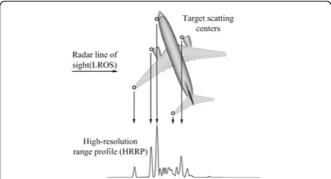
A high-resolution range profile (HRRP) is the amplitude of coherent summations of the complex time return from target scatterers in each range resolution cell, which represents the projection of the complex returned from the target scatting centers onto the line-of-sight (LOS), as shown in Figure 1. Since it contains the target structure signatures, such as target size and scatterer distribution, radar HRRP target recognition has received intensive attention from the radar automatic target recognition (RATR) community [1-16].
Several studies [8-16] show that statistical recognition is an efficient method for RATR. Figure 2 shows a typical flow chart of radar HRRP statistical recognition. By statis-tical recognition is meant the feature vectoryextracted from test HRRP samplexwill be assigned to the class with maximum posterior probabilityp(c|y), wherecÎ{1, ...,C} denotes the class membership. According to Bayes algo-rithm, p(c|y) ∝ p(y|c)p(c), where p(y|c) is the
class-conditional likelihood andp(c) is the prior class probabil-ity. Since the prior class probability is usually assumed to be uniformly distributed, estimation of the posterior prob-ability p(c|y) of each class is turned into estimation of the class-conditional likelihoodp(y|c) of each class. There are usually two stages (training and classification) in the statistical recognition procedure. We suppose the class-conditional likelihoodp(y|c) can be described via a model with a set of parameters (i.e., a parametric model). In the training phase, these parameters are estimated via training data (known as statistical modeling); and in the classifica-tion phase, as discussed above, given a test samplex, we first extract the feature vectoryfrom the test sample, then we calculate the class-conditional likelihoodp(y|c) for each targetc, finally, the test sample is associated with targetc’if c= arg maxc p(c|y). The focus of this article is on the feature extraction and statistical modeling.
Feature extraction from HRRP is a key step of our recognition system. One of the general feature extrac-tion methods is feature dimensionality reducextrac-tion [5]. This method is generally supervised, and some
* Correspondence: [email protected]
National Lab. of Radar Signal Processing, Xidian University, Xi’an, China
discriminative information may be lost during the dimensional reduction procedure. Another general fea-ture extraction method is feafea-ture transformation. The study given in [6] investigates various higher-order spec-tra, and shows that the power spectrum has the best recognition performance. Rather than just utilizing the frequency domain feature as in [6], this study exploits the spectrogram feature of HRRP data for combining both time domain and frequency domain features, which is a two-dimensional feature providing the varia-tion of frequency domain feature with time domain fea-ture. Some statistical models [8-16] are developed for HRRP-based RATR, of which [14-16] successfully uti-lized the hidden Markov model (HMM) for modeling the feature vectors from the HRRP sequence. Since the HRRP sample is a typical high-dimensional distributed signal, it is computationally prohibitive to build such a high-dimensional HMM for describing HRRP sequences directly. Therefore, to avoid this problem, some dimen-sionality reduction methods are utilized. For example, in [14,15], the relax algorithm is employed to extract the waveform constituents from the HRRP radar echoes, and then an HMM is utilized to characterize the fea-tures; in [16], a nonstationary HMM is utilized to char-acterize the following two features, i.e., the location information feature of scattering centers which are
extracted via the multirelax algorithm, and the moments of HRRP radar echoes. Nevertheless, some information contained in HRRP samples will be inevitably lost dur-ing the dimensional reduction procedure. Moreover, since multiple aspect-dependent looks at a single target are utilized in the classification phase, the angular velo-city of the target relative to the LOS of the radar is required to remain the same for the training and classi-fication phases, which can hardly be satisfied for a non-cooperative target.
The study reported here seeks an alternative way of exploiting HMM, in which we characterize the spectro-gram feature from a single HRRP sample via the hidden Markov structure. In our model, the spectrogram fea-ture extracted from each single HRRP is viewed as a
d-dimensional sequence (d is the length of spectrogram feature in the frequency dimension), thus only a single HRRP sample is required for the classification phase rather than an aspect-dependent sequence. The main contribution of this study can be summarized as follows.
(a) Spectrogram feature: The time domain HRRP samples only characterize the time domain feature of the target, which is too simple to obtain good per-formance. By contrast, the spectrogram feature introduced in this article is a time-frequency repre-sentation of HRRP data. The physical meaning of the spectrogram feature extracted from an HRRP sample is that the spectrogram feature in each time bin characterizes the frequency domain property of a fragment of the target, which can reflect the scatter-ing properties of different physical constructions. Therefore, the spectrogram feature should be a bet-ter choice for the recognition problem.
(b)Nonparametric model selection via stick-breaking construction:In the context of target recognition using HMMs, a key issue is to develop a methodol-ogy for defining an appropriate set of states to avoid over- or under-fitting. A Bayesian nonparametric infinite HMM (iHMM) which constituted by the hierarchical Dirichlet process (HDP) has proven Figure 1Illustration of an HRRP sample from a plane target,
where the scatters on the plane target are represented in circles. This figure is cited from [1].
effective to infer the number of states in acoustic sensing scenarios [17,18]. However, the lack of con-jugacy between the two-level HDP means that a truly variational Bayesian (VB) solution is difficult for HDP-HMM, which makes computationally pro-hibitive in large data problems. Recent study [19] proposes another way to constitute iHMM, where each row of transition matrix and initial state prob-ability is given with a fully conjugate infinite dimen-sional stick-breaking prior, which can accommodate an infinite number of states, with the statistical property that only a subset of these states will be used with substantial probabilities, referred to as the stick-breaking HMM (SB-HMM). We utilize the truncated version of such stick-breaking construc-tion in our model to characterize the HMM states, which is referred to as the truncated stick-breaking HMM (TSB-HMM).
(c)Multi-task learning (MTL):A limitation of statistical model is that it usually requires substantial training data, assumed to be similar to the data on which the model is tested. However, in radar target recognition problems, one may have limited training data. In addi-tion, the test data may be obtained under different motion circumstance. Rather than building models for each data subset associated with different target-aspect individually, it is desirable to appropriately share the information among these related data, thus offering the potential to improve overall recognition performance. If the modeling of one data subset is termed one learn-ing task, the learnlearn-ing of models for all tasks jointly is referred to as MTL [20]. We here extend the TSB-HMM learning in a multi-task setting for spectrogram feature-based radar HRRP recognition.
(d)Full Bayesian inference: We present a fully con-jugate Bayesian model structure, which does have an efficient VB solution.
The remainder of this article is organized as follows. We introduce spectrogram feature of HRRP data and analyze its advantages over time domain samples in Section 2. Sec-tion 3 briefly reviews the tradiSec-tional HMMs. In SecSec-tion 4, the proposed model construction is introduced, and the model learning and classification are implemented based on VB inference. We present experimental results on both single-task and multi-task TSB-HMM with time domain feature and spectrogram feature of measured HRRP data in Section 5. Finally, the conclusions are addressed in Section 6.
2. Spectrogram feature extraction
2.1 Definition of the spectrogram
The spectrogram analysis is a common signal processing procedure in spectral analysis and other fields. It is a
view of a signal represented over both time and fre-quency domains, and has widely been used in the fields of radar signal processing, and speech processing [21,22], etc.
Spectrograms can readily be created by calculating the short-time Fourier transform (STFT) of the time signal. The STFT transform may be represented as
STFT(τ,ω) =
∞
−∞x(u)w(u−τ)e
−jωudu (1)
where x(u) is the signal to be transformed,w(·) is the window function.
The spectrogram is given by the squared magnitude of the STFT function of the signal:
Y(τ,ω) =|STFT(τ,ω)|2 (2) From (1) and (2), we can see that the spectrogram function shows how the spectral density of signal varies with time.
In RATR problems, employing some nonlinear trans-formation (e.g., power transform metric) in feature domain may correct for the departures of samples from normal distribution to some extent and improve average recognition of learning models [2]. The power transform metric is defined as
y=xa; 0<a<1 (3) whereais the power parameter.
2.2 Spectrogram feature of HRRP data
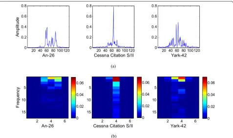
The sequential relationship across the range cells within a single HRRP echo can reflect the physical composition of the target. This can be illustrated by Figure 3, which presents the HRRP samples and corresponding spectro-gram features from three plane targets, i.e., Yark-42, An-26, and Cessna Citation S/II.
chunk or each range cell), the observation of a spectro-gram feature is a vector, while that of time domain fea-ture (HRRP sample) is a scalar. Thus, the high-dimensional feature vector may reflect more details than a single point for discrimination.
3. Review of traditional HMM: finite HMM and infinite HMM
The HMM [24] has widely been used in speech recogni-tion and target recognirecogni-tion. It is a generative representa-tion of sequential data with an underlying markovian process selecting state-dependents distributions, from which observations are drawn. Specially for a sequence of lengthT, a state sequences= (s1,s2, ...,sT) is drawn from
P(st|st-1). Given the observation modelf(·), the observa-tion sequencex = (x1,x2, ...,xT) can then be drawn as
f(θst), whereθst is a set of parameters for the observation models which is indexed by the state at timet.
An HMM can be modeled as F = {w0, w, θ}, each
parameter is defined as
w0={w0,i}, w0,i= Pr(s1=i) : Initial state distribution
w={wi,j}, wi,j= Pr(st+1=j|st=i) : State transition probability θ={θi}, xt∼f(θst) : Emission likelihood
(4)
Given model parameters F, the probability of the
complete data can be expressed as
p(x,s|) =w0,i T−1
t=1
wst,st+1
T
t=1
p(xt|θst) (5)
And the data likelihood p(x|F) can be obtained by integrating over the states using the forward algorithm [24]. In a classical HMM [24], the number of the states with the HMM is initialized and fixed. There-fore, we have to specify model structure before learn-ing. However, in many practical applications, it needs an expansive model selection process to obtain a cor-rect model structure. To avoid the model selection process, a fully nonparametric Bayesian approach with countably infinite state spaces is employed, first pro-posed by Beal, and termed infinite Markov model (iHMM) [25].
Recent study [19] proposes the iHMM with stick-breaking priors (SB-HMM), which can be used to develop an HMM with an unknown number of states. In this model, each row of the infinite state transition matrix wis given a stick-breaking prior. The model is expressed as follows
Gi= ∞
j=1
wi,jδ(θj), wi,j=vi,j j−1
h=1
(1−vi,h), vi,j|βi∼Beta(1,βi)
βi∼Ga(aα,bα), θj∼H; i= 1, 2,· · · ∞; j= 1, 2,· · ·,∞
(6) 20 40 60 80 100120
0 0.2 0.4 0.6 0.8
An-26
Am
pl
itu
de
20 40 60 80 100120 0
0.2 0.4 0.6 0.8
Cessna Citation S/II
20 40 60 80 100120 0
0.2 0.4 0.6 0.8
Yark-42
(a)
An-26
F
requenc
y
2 4 6
5
10
15
0 0.02 0.04 0.06
Cessna Citation S/II
2 4 6
5
10
15
0 0.02 0.04 0.06
Yark-42
2 4 6
5
10
15
0 0.02 0.04 0.06
(b)
where the mixture distributionGi has weights repre-sented aswi = [wi, 1, wi, 2, ...,wi, j, ...], δ(θj) is a point
measure concentrated atθj, Beta(1, bi) represents the
Beta distribution with hidden variablebi, the drawn
vari-ables {vi,j}∞j=1 are independent and identically distributed (i.i.d), Ga(aa, ba) represents the Gamma distribution with preset parameters aa, ba, and H denotes a prior distribution from which the set {θj}∞j=1 is i.i.d drawn.
The initial state probability mass function, w0, is also constructed according to an infinite stick-breaking con-struction. Whenwiterminates at some finite numberI
-1 with wi,I ≡1− I−1
J=1wi,j, this result is a draw from a
general Dirichlet distribution [26], which is denoted as
wi~GDD(1(I-1) × 1, [bi](I-1) × 1), where1(I-1) × 1denotes an (I- 1)-length vector of ones, [bi](I-1) × 1is an (I- 1)-length vector ofbi, andIrepresents the truncation
num-ber of states.
The key advantage of stick-breaking construction is
that the corresponding state-dependent parametersθj
are drawn separately, effectively detaching the construc-tionθfrom the construction initial-state probability w0 and state transition matrixw. This is contrast with HDP priors [27], where these matrices are linked with two-level construction. Therefore, the stick-breaking con-struction makes fast variational inference feasible. In addition, the SB-HMM has a good sparse property, which promotes a sparse utilization of the underlying states [19].
4. The SB-HMM for HRRP data
4.1 MTL model construction
According to the scattering center model [4], for a high-resolution radar system, a radar target does not appear as a“point target”any more, but consists of many scatterers distributed in some range cells along radar LOS. For a cer-tain target, the scattering center model varies throughout the whole target-aspect. Therefore, pre-processing techni-ques should be applied to the raw HRRP data. In our pre-vious work [11-13], we divide the HRRP into frames according to the aspect-sectors without most scatterers’ motion through resolution cells (MTRC), and use distinct parametric models for statistical characterization of each HRRP frame, which are referred to as the aspect-frames and corresponding single-task learning (STL) models in our articles.
For the motivating HRRP recognition problems of interested here, we utilize TSB-HMM for analyzing spectrogram features extracted from HRRP data. For a multi-aspect HRRP sequence of target c(c Î{1, ..., C} with Cdenoting the number of targets here), we divide the data intoMcaspect frames, e.g., themth set (herem
Î {1, ..., Mc}) is {x(c,m,n)}Nn=1 where N denotes the
number of samples in the frame, andx(c, m, n)= [x(c, m,
n)
(1), ...,x(c, m, n)(Lx)]Trepresents thenth HRRP sample
in themth frame, withLxdenoting the number of range
cells in an HRRP sample. Each aspect frame corresponds to a small aspect-sector avoiding scatters’ MTRC [13], and the HRRP samples inside each target-aspect frame can be assumed to be i.i.d. We extract the spectrogram feature of each HRRP sample, andY(c, m, n)= [y(c, m, n) (1), ...,y(c, m, n)(Ly)] denotes the spectrogram feature ofx
(c, m, n)
as defined in (2) withLydenoting the number of
time bins in spectrogram feature.
If learning a separate TSB-HMM for each frame of the target, i.e., {Y(c,m,n)}N
n=1, is termed the single-task
HMM (STL HMM). Here, we wish to learn a TSB-HMM for all the aspect-frames (tasks) of one target jointly, which is referred to as multi-task TSB-HMM (MTL TSB-HMM). MTL is an approach to inductive transfer that improves generalization by using the domain information contained in the training samples of related tasks as an inductive bias [20]. In our learning problems, the aspect-frames of one target may be viewed as a set of related learning tasks. Rather than building models for each aspect-frame individually (due to target-aspect sensitivity), it is desirable to appropri-ately share the information among these related data. Therefore, the training data for each task are strength-ened and overall recognition performance is potentially improved.
The construction of the MTL TSB-HMM with para-meters for targetcis represented as
y(c,m,n)(l)∼f(θ s(c,m,n)
l ); l= 1,. . .,Ly; n= 1,. . .,N; m= 1,. . .,Mc; s(lc,m,n)∼
⎧ ⎨ ⎩
w(0c,m)if l= 1
w(c,m) s(c,m,n) l−1
if l≥2
w(ic,m)|βi∼GDD(1(I−1)×1, [βi](I−1)×1), βi|aα,bα∼Ga(aα,bα); i= 0,. . .,I
θi∼H; i= 1,. . .,I
(7)
where y(c, m, n)(l) islth time chunk of nth sample’s spectrogram in the mth aspect-frame of thecth target,
s(lc,m,n) denotes the corresponding state indicator, (aa, ba) are the preset hyperparameters. Here, the observa-tion modelf(·)is defined as independently normal
distri-bution, and each corresponding element in H(·) is
The main difference between MTL TSB-HMM and STL TSB-HMM is in the proposed MTL TSB-HMM, all the multi-aspect frames of one target are learned jointly, each of theMc tasks of targetc is assumed to have an
independent transition statistics, but the state-dependent observation statistics are shared across these tasks, i.e., the observation parameters are learned via all aspect-frames; while in the STL TSB-HMM, each multi-aspect frame of targetc is learned separately, therefore, each target-aspect frame builds its own model and the corresponding parameters are learned just via this aspect-frame.
4.2 Model learning
The parameters of proposed MTL TSB-HMM model are treated as variables, and this model can readily be implemented by Markov Chain Monte Carlo (MCMC) [28] method. However, to approximate the posterior dis-tribution over parameters, MCMC requires large com-putational resources to assess the convergence and reliability of estimates. In this article, we employ VB inference [19,29,30], which does not generate a single point estimation of the parameters, but regard all model parameters as possible, with the goal of estimating the posterior density function on the model parameters, as a compromise between accuracy and computational cost for large-scale problems.
The goal of Bayesian inference is to estimate the
pos-terior distribution of model parameters F. Given the
observation data X and hyper parametersg, by Bayes’ rule, the posterior density for the model parameters may be expressed as
p(|X,γ) = p(X|,γ)p(|γ)
p(X|,γ)p(|γ)d (8)
where the denominator ∫p(X|F,g)p(F|g)dF=p(X|g) is the model evidence (marginal likelihood).
VB inference provides a computationally tractable way which seeks a variational distribution q(F) to approxi-mate the true posterior distribution of the latent vari-ablesp(F|X,g), we obtain the expression
logp(X|γ) =L(q()) +KL(q()||p(|X,γ)) (9)
where L(q()) =
q() logp(X|,γ)p(|γ)
q() d, and
KL(q(F)||p(F|X, g)) is the Kullback-Leibler (KL) diver-gence between the variational distributionsq(F) and the true posteriorp(F|X,g). SinceKL(q(F)||p(F|X, g))≥0, and it reaches zero whenq(F) =p(F|X, g), this forms a lower bound for logp(X|g), so we have logp(X|g)≥L(q
(F)). The goal of minimizing the KL divergence between the variational distribution and the true posterior is
i E
( , )c m
W
I
I
i T
H
( , , )c m n l
s
( , , )c m n l
y
,
a bD D
,y
N L
c
M
( , ) 0
c m w
( , )c m
i w
I
I i
T H
( , , ) 1
c m n
s ( , , )
2
c m n
s ( , , )
3
c m n
s ( , , )c m n
L
s
( , , ) 1c m n
y ( , , )
2c m n
y ( , , )
3c m n
y ( , , )c m n
L y
(a) (b)
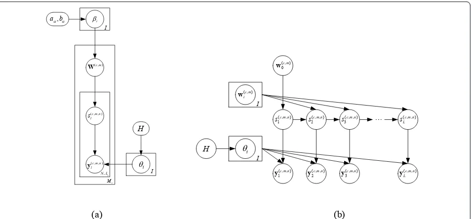
Figure 4Graphical representation of the MTL TSB-HMM, the detailed generative process is described in (7).(a)Graph of the MTL
TSB-HMM, the detailed generative process is described in (6). Here, W(c,m)= [w(c,m)T
0 ;w
(c,m)T
1 ;. . .;w (c,m)T
I ],iis the state index,cis the target
equal to maximize this lower bound, which is known as the negative free energy in statistical physics.
For the computational convenience and intractable of the negative-free energy, we assume a factorizedq(F),
i.e., q() =
k
qk(ϕk), which has same form as
employed inp(F|X, g). With this assumption, the mean field approximation of the variational distributions for
the proposed MTL TSB-HMM with target c may be
expressed as
q() =
Mc m=1 I i=0
q(w(ic,m))[
Mc m=1 N n=1 Ly l=1
q(s(lc,m,n))]q(θ)q(β)(10)
where {{w(ic,m)}Mc,I m=1,i=0,{s
(c,m,n)
l }
Mc,N,Ly
m=1,n=1,l=1,θ,β} are the
latent variables in this MTL model.
A general method for performing variational infer-ence for conjugate-exponential Bayesian networks out-lined in [17] is as follows: for a given node in a graphic model, write out the posterior as though everything were known, take the logarithm, the expectation with respect to all known parameters and exponentiate the result. We can implement expectation-maximization (EM) algorithm in variational inference. The lower bound is increased in each of iteration until the algo-rithm converges. In the following experiments, we ter-minate EM algorithm when the changes of the lower bound can be neglected (the threshold is 10-6). Since it requires computational resource comparable to EM algorithm, variational inference is faster than MCMC methods. The detailed update equations for the latent variables and hyperparameters of MTL TSB-HMM with HRRP spectrogram feature are summarized in the Appendix.
4.3 Main procedure of radar HRRP target recognition based on the proposed MTL TSB-HMM algorithm
The main procedure of radar HRRP target recognition based on the proposed MTL TSB-HMM algorithm is shown as follows.
4.3.1. Training phase
(1) Divide the training samples of target c(c= 1, 2, ..., C) into HRRP frames {x(c,m)}Mc
m=1, where Mc is the
number of tasks of target c, x(c,m)={x(c,m,n)}N n=1
denotes the mth range aligned and amplitude
nor-malized HRRP frame, N is the number of echoes a
frame contains.
(2) Extract the spectrogram feature {Y(c,m,n)}Mc,N m=1,n=1
of each HRRP sample with Y(c, m, n)= [y(c, m, n)(1),y (c, m, n)
(2), ...,y(c, m, n)(Ly)] denoting the spectrogram
feature ofx(c, m, n)as defined in (2).
(3) For each target, we construct an MTL
TSB-HMM model, and learn the parameters of w(c,m)
0,s(1c,m)
,
w(i,cj,m), andθifor all aspect-frames of the target via
using spectrogram feature, where w(c,m)
0,s(1c,m)
is the
initial state probability for the index framemof tar-getc, w(i,cj,m) is state transition probability from state
ito the j for the index frame mof target c, and θi
are the parameters of observation model associated with corresponding statei(cÎ {1, ...,C},mÎ{1, ...,
Mc}, i, jÎ{1, ..., I}). The detailed learning procedure
of the parameters of MTL TSB-HMM with HRRP spectrogram feature are discussed in Section 4.3 and the Appendix.
(4) Store the parameters of initial state probability
w(c,m)
0,s(1c,m)
Mc
m=1
, state transition probability w(c,m)Mc m=1
and the parameters of observation model {θi}Ii=1 for
each targetcwithc= 1, 2, ...,C.
4.3.2. Classification phase
(1) The amplitude normalized HRRP testing sample is time-shift compensated with respect to the aver-aged HRRP of each frame model via the slide corre-lation processing [23].
(2) Extract the spectrogram feature Y(testc,m)C,Mc c=1,m=1of
the slide-correlated HRRP testing samplextest, where Y(testc,m)={[y
(c,m)
test (1),y
(c,m)
test (2),. . .,y (c,m)
test (Ly)]} denotes the spectrogram feature of HRRP testing sample cor-related withmth frame of target cas defined in (2). (3) The frame-conditional likelihood of target can be calculated as
p(Y(testc,m)|c,m) =
s
w(c,m)
0,s(c,m) 1
Ly
l=2
w(c,m) s(c,m)
l−1,s (c,m) l
Ly
l=1
f(c,m)(y(c,m) test (l)|
θs(c,m) l
) (11)
where〈·〉 means the posterior expectation for the latent variable over the corresponding distribution
on it, e.g.,
w(c,m)
0,s(1c,m)
denotes the posterior
expecta-tions of initial state probability,
w(c,m)
sl(−c,1m),s(lc,m)
denotes
the posterior expectations of state transition
prob-ability from state s(l−c,m1) to the s(lc,m) for the frame m
of targetc, and
θs(c,m)
l
denotes the posterior
associated with state s(lc,m), with the corresponding
state indicator for the lth time chunk
s(lc,m)∈ {1,· · ·,I}. Then, p(Y(testc,m)|c,m) can be calcu-lated by forward-backward procedure [24] for each
m(mÎ{1, ...,Mc}) andc(cÎ{1, ...,C}).
(4) We calculate the class-conditional likelihood
p(Y(testc)|c) for each targetc
p(Y(testc)|c) = arg max m p(Y
(c,m)
test |c,m); m= 1,. . .Mc (12)
(5) As discussed in Section 1, the testing HRRP sam-ple will be assigned to the class with the maximum class-conditional likelihood, with the assumption that the prior class probabilities are same for all tar-gets of interests,
k= arg max c p(Y
(c)
test|c); c= 1,· · ·,C (13)
5. Experimental results
5.1 Measured data
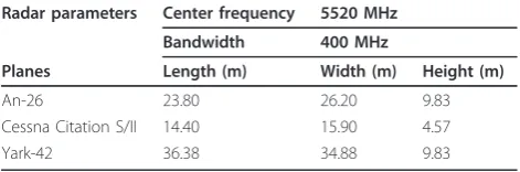
We examine the performance of the TSB-HMM on the 3-class measured data, including three actual aircrafts (a propeller plane An-26, a small yet plane Cessna Citation S/II, and a big yet plane Yark-42), the radar works on a
Cband with bandwidth of 400 MHz, the range
resolu-tion of the HRRP is about 0.375 m.
The parameters of the targets and radar are shown in Table 1, and the projections of target trajectories onto the ground plane are displayed in Figure 5, from which the aspect angle of the airplane can be estimated according to its relative position to radar. As shown in Figure 5, all aspects of targets were measured repeatedly several times in this dataset. The requirements of choos-ing trainchoos-ing data and test data are that the trainchoos-ing data and the test data are from different data segments, and the training data cover almost all of target-aspect angles of the test data, but their elevation angles are different. The second and the fifth segments of Yark-42, the sixth and the seventh segments of Cessna Citation S/II and the fifth and the sixth segments of An-26 are taken as the training samples while the remaining data are left
for testing. These training data almost cover all of the target-aspect angles. Also, we need test data from differ-ent target to measure the rejection performance of our model. Here, we use 18,000 truck HRRP samples gener-ated by the electromagnetic simulator software, XPATCH, as a confuser target. In addition, the HRRP samples are 128-dimensional vectors.
As discussed in the literature [11,12], it is a prerequisite for radar target recognition to deal with the target-aspect, time-shift, and amplitude-scale sensitivity. According to radar parameters and the condition of aspect sectors without MTRC, for training data from 3 targets we totally have 135 HRRP frames, of which 35 from Yark-42, 50 from Cessna Citation S/II and 50 from An-26. Similar to the previous study [11-13], HRRP training samples should be aligned by the time-shift compensation techni-ques in ISAR imaging [23] to avoid the influence of time-shift sensitivity. Each HRRP sample is normalized byL2 normalization algorithm to avoid the amplitude-scale sensitivity. In the rest of the article, the training HRRPs in each frame are assumed to have been aligned and normalized.
Nine training datasets are considered for training: 1 × 135, 2 × 135, 4 × 135, 8 × 135, 16 × 135, 32 × 135, 64 × 135, 128 × 135 and 1024 × 135, where 2 × 135 means 2 HRRP samples randomly selected from each of the 135 target-aspect frames, i.e., there are totally 2 × 135 = 270 HRRP training samples, similar meaning for other size of HRRP datasets. Since MTL needs load the whole HRRP training dataset of a target to share the information among them, it requires more memory resource than STL. Due to the limited memory resource of our computer, we do not consider 1024 × 135 training dataset in MTL. Since there is no prior knowledge about how many states we should use, and how to set these states, the HMM states are not manually set like [31]. We set a large truncation number in our model to learn the meaningful states auto-matically. In the following experiments, we set the trunca-tion levelIto 40 for both spectrogram feature and time domain feature in STL, andIto 60 for both spectrogram feature and time domain feature in MTL. Similar results were found for lager truncations. In our model, since the parameterbicontrols the prior distribution on the number
of states, we set the hyper-parametersaa=ba= 10-6for eachbito promote sparseness on states.
5.2 Time domain feature versus spectrogram feature
In this experiment, STL HMM and MTL TSB-HMM of HRRP training datasets within each frame are learned, respectively, and the two features, i.e., time domain and spectrogram features, are compared. When using the HRRP time domain feature, we can just sub-stitute the scalar x(c, m, n)(l) for the vectory(c, m, n)(l) in (6), where x(c, m, n)(l) represents thenth HRRP sample
Table 1 Parameters of planes and radar in the experiment
Radar parameters Center frequency 5520 MHz
Bandwidth 400 MHz
Planes Length (m) Width (m) Height (m)
An-26 23.80 26.20 9.83
Cessna Citation S/II 14.40 15.90 4.57
in themth frame of target c, withldenoting the corre-sponding range cell in the HRRP sample.
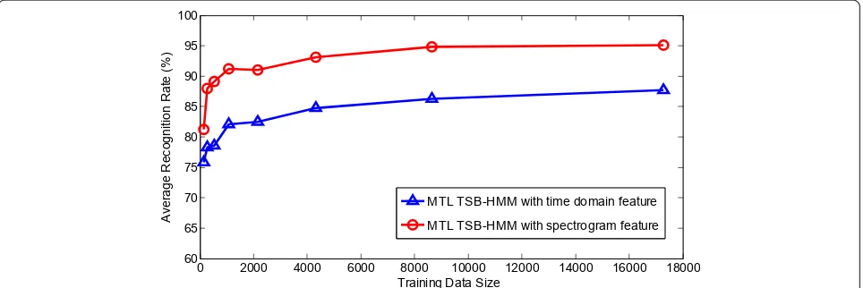
Figure 6 shows that the performances of STL TSB-HMMs based on time domain feature are better than those based on spectrogram feature when training data-set no more than 32 × 135. The reason is that more parameters need to be estimated for the model with spectrogram feature than that with time domain feature. For example, for a target-aspect frame with 32 training samples, we need to estimate the 40 16-dimensional states for the model with spectrogram feature; while 25 1-dimensional states for the model with time domain feature. When training data size larger than 32 × 135, spectrogram feature obtains obviously better perfor-mance. Table 2 further compares the confusion matrices and average recognition rates of using time domain fea-ture and spectrogram feafea-ture with 1024 × 135 training samples via STL. We can clearly find that the average recognition rate obtained by spectrogram feature is about 6.6% points larger than that obtained by the time domain feature. The performances of MTL TSB-HMMs are shown in Figure 7. Since MTL sharing states between different tasks of a target, which is better for
parameter learning with small training data size, spec-trogram domain feature outperforms time domain fea-ture even with few training data.
The posterior state distributions of MTL TSB-HMM with spectrogram feature for all the three plane targets with 128 × 135 training data are shown in Figure 8. In this example, the state truncation level ofI= 60 is employed for each plane. Further for each plane, the 60 hidden states are shared across all aspect-frames, and there are 46, 48, and 49 meaningful states with the posterior state usage larger than zero for Yark-42, Cessna Citation S/II, and An-26, respectively, and those of other 14, 12, and 11 states are zero, which justifies using the truncated version stick-breaking prior for our data.
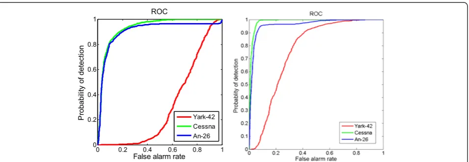
Next, we consider the target rejection problem. Three planes targets are considered as“in-class targets”, while the simulated data consists of 18,000 truck HRRP sam-ples are considered as confuser targets. Two examsam-ples of confuser targets HRRP samples are shown in Figure 9. Our goal is to test whether a new data is in the family of the in-class targets or not. Figure 10 presents the rejec-tion performance evaluated by the receiver operarejec-tion characteristic (ROC) curves. The ROC curve depicts the
-200 -15 -10 -5 0
5 10 15 radar 1 2 3 3 4 5 6 7 Km
˄a˅An-26
K
m
-200 -15 -10 -5 0
5 10 15 radar 1 2 3 4
5 7 6
Km
˄b˅ Cessna
K
m
-5 0 5 10
0 20 40 60 80 radar 1 2 3 4 5 Km
˄c˅Yark-42
K
m
Figure 5Projections of target trajectories onto the ground plane: (a) An-26.(b)Cessna Citation S/II.(c)Yark-42.
-200 -15 -10 -5 0 5 10 15 radar 1 2 3 3 4 5 6 7 Km
˄a˅An-26
Km
-200 -15 -10 -5 0 5 10 15 radar 1 2 3 4 5 7 6
Km
˄b˅ Cessna
Km
-5 0 5 10
0 20 40 60 80 radar 1 2 3 4 5 Km
˄c˅Yark-42
Km
0 2 4 6 8 10 12 14
x 104
30 40 50 60 70 80 90 100
Training Data Size
A vera ge R ec ogn iti on R at e (% )
STL TSB-HMM with time domain feature STL TSB-HMM with spectrogram feature
detection probability versus the false alarm probability. For a fixed false alarm probability, a method with the higher detection probability is better. The dataset size is selected as 128 × 135 in the training phase. The ROC curves are shown in Figure 10. The spectrogram based TSB-HMMs outperforms the time domain feature-based TSB-HMMs, especially for Yark-42. Figure 11 shows the test likelihoods of 1,200 Yark-42 samples and 18,000 confuser target samples obtained with STL TSB-HMM. As shown in Figure 11a, when using the time domain feature, the test likelihoods of Yark-42 samples are relative low, and many confuser samples have higher test likelihoods than Yark-42 samples. That is to say, when we set a high discrimination threshold, the detec-tion probability is very low, and the false alarm probabil-ity is high. By contrast, from Figure 11b, we can find that when using the spectrogram feature, the test likelihoods of Yark-42 samples are higher than most of the test likeli-hoods of the confuser samples. Therefore, the detection performance of the spectrogram feature is much better than that of the time domain feature for Yark-42.
5.3 STL versus MTL
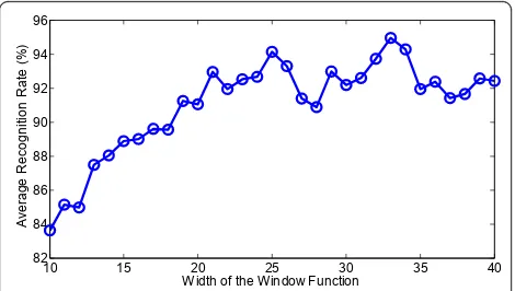
In order to model spectrogram feature, two parameters need to be set first, i.e., the width of window function and the length of the overlapped window.
In the feature space, the spectrogram varies with the width of the window function and the overlap across the windows. For HRRP data analysis, a wide window function provides better frequency resolution, but wor-sens the time resolution, and vice versa. Physically, since the width of a window function determines the length of segments of a target, the longer the segment we divide a target into, the more physical composition of the target will be contained in the each component of the observation vector; meanwhile, the overlap across the windows determines the redundancy of the segments.
We build a set of MTL TSB-HMMs to search these two parameters. The width of the window function is chosen from 10 to 40 range cells with an increment of 1 range cells, and the overlap length is fixed as typically half width of the window function. In this experiment, we use 64 × 135 training samples. As demonstrated in Figure 12, the optimal width of the window function is 33 range cells. We then fix the optimal window function width, and set the overlap length from 1 range cell to 29 range cells to determine the optimal overlap length. From Figure 13, the optimal overlap length is 16 range cells. Therefore, we extract the spectrogram feature with the window function width of 33 range cells and the overlap length of 16 range cells for training.
Table 2 Confusion matrices and average recognition rates of time domain feature and spectrogram feature based on STL TSB-HMMs with 1,024 training samples per target-aspect frame
1024 × 135 training samples Time domain feature Spectrogram feature
An-26 Cessna Citation S/II Yark-42 An-26 Cessna Citation S/II Yark-42
An-26 90.8 9.8 3.5 97.3 1.1 1.2
Cessna citation S/II 8.7 83.0 2.0 1.1 92.8 0.8
Yark-42 0.5 7.2 94.5 1.6 6.1 98.0
Average recognition rates (%) 89.4 96.0
-200 -15 -10 -5 0 5
10 15
radar 1 2
3 3 4
5
6 7
Km
˄a˅An-26
Km
-200 -15 -10 -5 0 5
10 15
radar 1
2
3 4 5 7 6
Km
˄b˅ Cessna
Km
-5 0 5 10
0 20 40 60 80
radar
1 2
3 4 5
Km
˄c˅Yark-42
Km
0 2000 4000 6000 8000 10000 12000 14000 16000 18000
60 65 70 75 80 85 90 95 100
Training Data Size
A
ve
rag
e
R
ec
og
ni
tion
R
at
e (%
)
MTL TSB-HMM with time domain feature MTL TSB-HMM with spectrogram feature
We compare two methods for spectrogram feature based TSB-HMM: (i) the proposed MTL TSB-HMMs method, for which we learn target-aspect frames of a target collectively; (ii) the STL TSB-HMMs method, for which each target-aspect frame of targets modeled
separately. As shown in Figure 14, the proposed MTL TSB-HMMs method consistently outperforms the STL TSB-HMMs method and the improvement is more sig-nificant when there is only a small amount of training data available. This is because MTL exploits the sharing states between different tasks and uses the sharing infor-mation to enhance the overall performance. In addition, in the state truncation level of I= 60 is employed for each of the three planes. For each plane, the 60 states are shared across the aspect-frames. Therefore, we only impose 60 × 3 = 180 states in the MTL TSB-HMMs. However, in the training phase of STL model, the state truncation level ofI= 40 is employed for each aspect-frame. As discussed in Section 5.1, we have 50 + 50 + 35 = 135 aspect-frames from the three targets. There-fore, we totally impose 40 × 135 = 5400 states in the STL TSB-HMMs. Table 3 summarizes the confusion
0 10 20 30 40 50 60
0 0.5
1 Yark-42
State Index
P
ro
ba
bi
lity
0 10 20 30 40 50 60
0 0.5 1
State Index
P
ro
ba
bi
lity
Cessna Citation S/II
0 10 20 30 40 50 60
0 0.5 1
State Index
P
ro
ba
bi
lity
An-26
Figure 8The hidden state distributions for all the three plane targets with 128 × 135 training data, generated via a run of the MTL TSB-HMM with spectrogram feature. In this example, the state truncation level ofI= 60 is employed for each plane. For each plane, 60 hidden states are shared across all aspect-frames, and 46, 48, and 49 meaningful states are inferred for Yark-42, Cessna Citation S/II, and An-26, respectively.
0
50
100
0
0.2
0.4
0.6
Am
p
lit
ud
e
0
50
100
0
0.2
0.4
0.6
0 0.2 0.4 0.6 0.8 1 0
0.2 0.4 0.6 0.8 1
False alarm rate
P
robabi
lit
y o
f det
ec
tion
ROC
Yark-42 Cessna An-26
0 0.2 0.4 0.6 0.8 1
0 0.2 0.4 0.6 0.8 1
False alarm rate
P
rob
abi
lit
y of
d
et
ec
tio
n
ROC
Yark-42 Cessna An-26
(a) (b)
Figure 10Rejection results for different sets of targets using STL TSB-HMMs with different features.(a)STL TSB-HMM with time domain feature (average AUC: 0.738).(b)STL TSB-HMM with spectrogram feature (Average AUC: 0.924).
0
2000
4000
6000
8000 10000 12000 14000 16000 18000
100
150
200
Test Sample Index
Log Li
kel
ihood
Confuser Targets
Yark-42
(a)
0
2000
4000
6000
8000 10000 12000 14000 16000 18000
100
200
300
400
500
600
Test Sample Index
Log
Li
ke
lih
oo
d
Confuser Targets
Yark-42
(b)
matrix and average recognition performance of STL TSB-HMMs and MTL TSB-HMMs, with 2 × 135 and 128 × 135 training samples. Note that when we only use 2 × 135 samples for training, the average recognition rate of STL TSB-HMMs is only 52.7%, while the average recognition rate of MTL TSB-HMMs is 88.0%. With the training data increasing, the performance of STL becomes close to that of MTL. The average recognition rate obtained by MTL is about 2.3% higher than that by STL for 128 × 135 training samples.
We also consider the target rejection problem here. The ROC curves of MTL TSB-HMMs are presented in Figure 15. Compare with Figure 10, the area under curve (AUC) of STL are slightly larger than that of MTL.
5.4 MTL with power transformed spectrogram feature
We employ the power transform metric for all the observation vectors (the vectors in each fixed time) of the spectrogram. Figure 16 show that the optimal
para-meter a* = 0.4. Figure 17 shows the performance of
MTL TSB-HMMs is better than STL-HMMs for power transformed spectrogram feature. Compared with the average recognition rate of original spectrogram feature in Figure 14, that of power transformed spectrogram feature shown in Figure 17 are much larger, especially for small training data sets.
The confusion matrix and average recognition rates of STL TSB-HMMs and MTL TSB-HMMs with power transformed spectrogram feature are shown in Table 4, where 2 × 135 and 128 × 135 training samples are used for learning the models. Note that, when we consider 2 × 135 training samples for MTL TSB-HMMs based on spectrogram feature with the optimal power transforma-tion, the average of recognition rate is nearly equivalent to the case of considering 128 × 135 training samples for that based on original spectrogram feature. When using 128 training samples per target-aspect frame for STL TSB-HMMs, the average recognition rate is gained by 4.3% via power transformation; while for MTL TSB-HMMs the gain is 2.5%.
Similarly, as shown in Figure 18, we obtained the ROC curve for power transformed spectrogram feature in the same experimental environment as that we mentioned in Section 5.3. The AUC of STL and MTL with trans-formed spectrogram features are gained by 3.3 and 5.0%; therefore, the model of using the transformed spectro-gram features can improve the rejection performance.
5.5 Computation burden
All experiments have been performed in nonoptimized programme written in Matlab, on a Pentium PC with 3.2-GHz CPU and 2 GB RAM. In our VB algorithm, when the relative change of lower bound between two consecutive iterations is less than the threshold 10-6, we believe our algorithm converges. Generally, in a practical application, the larger training dataset requires the huger computational burden in the training phase. When the training dataset contains 128 × 135 training samples, the VB algorithm of the MTL TSB-HMM with
time domain feature and the truncation numberI= 60
converges after about 400 iterations and requires about 14 h, and the VB algorithm of MTL TSB-HMMs with
spectrogram feature and the truncation number I= 60
converges after about 200 iterations and requires about 2 h. Although the above computation is pretty expen-sive, we know that the computation cost in the training phase can be ignored for an off-line learning (or train-ing) system, and it is more important to evaluate the computation cost in the classification phase. The MTL TSB-HMMs with time domain feature and spectrogram feature require 0.6680 and 1.5893 s, respectively, to match a test sample with all frame models. The compu-tation time given here is averaged over ten runs.
10 15 20 25 30 35 40
82 84 86 88 90 92 94 96
Width of the Window Function
A
ver
age
R
eco
gn
iti
on
R
a
te
(
%
)
Figure 12 Recognition rates of spectrogram features with different width of the window function via MTL TSB-HMMs. The overlap length is fixed as typically half width of the window function.
10 12 14 16 18 20 22 24 26 28
86 87 88 89 90 91 92 93 94 95
Overlap Length
A
ver
ag
e
R
ec
o
gn
iti
on
R
a
te
(
%
)
Figure 14Average recognition rates of the STL TSB-HMMs and MTL TSB-HMMs with spectrogram feature versus the number of training samples.
Table 3 Confusion matrices and average recognition rates of spectrogram feature based on STL TSB-HMMs and MTL TSB-HMMs with 2 training samples and 128 training samples per target-aspect frame
STL TSB-HMMs MTL TSB-HMMs
An-26 Cessna Citation S/II Yark-42 An-26 Cessna Citation S/II Yark-42
2 × 135 training samples
An-26 81.0 87.0 14.1 86.3 1.3 4.9
Cessna citation S/II 8.0 3.5 12.2 12.2 88.0 5.4
Yark-42 11.0 9.5 73.7 1.5 10.7 89.7
Average recognition rates (%) 52.7 88.0
128*135 training samples
An-26 93.8 0.7 2.5 95.8 0.4 1.9
Cessna citation S/II 4.4 88.3 1.1 3.5 92.3 0.8
Yark-42 1.8 11.0 96.4 0.7 7.3 97.3
Average recognition rates (%) 92.8 95.1
0 0.2 0.4 0.6 0.8 1
0 0.2 0.4 0.6 0.8 1
False alarm rate
P
ro
ba
bilit
y o
f d
et
ec
tio
n
ROC
Yark-42 Cessna An-26
6. Conclusion
We have utilized spectrogram feature of HRRP data and presented an MTL-based hidden Markov model with truncated stick-breaking prior (MTL TSB-HMM) for radar HRRP target recognition. The construction of this model allows VB inference, which extremely decreases the computational burden.
After resolving the three sensitivity problems, i.e., the target-aspect, time-shift, and amplitude scale sensitivity of HRRP, respectively, we first compare the spectrogram feature of HRRP with the time domain feature of HRRP data via single-task and multi-task learning-based hid-den Markov model with truncated stick-breaking prior (STL and MTL TSB-HMM). Second, we measure the
0.1 0.2 0.3 0.4 0.5 0.6 0.7 0.8 0.9 1
94.5 95 95.5 96 96.5 97 97.5 98
Power Index
Av
era
ge
R
ec
o
gn
iti
on
R
a
te
Figure 16Average recognition rate of spectrogram features with different power transformed via MTL TSB-HMMs.
Figure 17Average recognition rates of the STL TSB-HMMs and MTL TSB-HMMs with spectrogram feature transformed by optimal power (0.4) versus the number of training samples.
Table 4 Confusion matrices and average recognition rates of power transformed spectrogram feature (power
parameter is 0.4) based on STL TSB-HMMs and MTL TSB-HMMs with 2 training samples and 128 training samples per target-aspect frame
STL TSB-HMMs MTL TSB-HMMs
An-26 Cessna Citation S/II Yark-42 An-26 Cessna Citation S/II Yark-42
2 × 135 training samples
An-26 90.4 5.3 42.3 95.8 1.4 5.0
Cessna Citation S/II 9.4 93.0 34.5 3.9 96.7 5.0
Yark-42 0.2 1.7 23.2 0.3 1.9 90.0
Average recognition rates (%) 68.9 94.2
128 × 135 training samples
An-26 99.2 3.3 1.2 98.9 1.2 1.4
Cessna Citation S/II 0.4 94.3 1.0 0.9 96.0 0.6
Yark-42 0.4 2.4 97.8 0.2 2.8 98.0
performance of STL TSB-HMM and MTL TSB-HMM with spectrogram feature, where in MTL TSB-HMM, the multiple tasks are linked by different target-aspects. Finally, we introduce power transformation metric to improve the recognition performance of spectrogram feature. It is shown that using spectrogram feature not only have a better ROC, but also obtain a better recog-nition performance than using HRRP time domain fea-ture. MTL shares the underlying state information among different target-aspects, and can provide a better recognition performance compared to STL. In addition, the power transformation metric can enhance both aver-age recognition rate and ROC. It is worth to point out that our MTL model with spectrogram feature can obtain a good recognition performance with much fewer training data compared with the conventional radar HRRP-based statistical recognition methods, which is a good property for RATR.
Appendix
Derivation of update equations in VB approach
1. Updateq(θi):
For the MTL TSB-HMM model introduced in Section 4.3 and the corresponding mean-field variational distri-bution described in (9), q(θi) is defined by the specific
application:
logq(θi)∝logH(θi|˜θi) + Mc m=1 N n=1 Ly l=1
<s(l,ci,m,n)>logf(y(c,m,n)(l)|θ
i) i= 1,. . .,I (14)
where q(θi) is defined by the specific application, and
˜
θi denotes the parameters in the q(θi), <sl(,ci,m,n)>
represents the expected number of state indicator
s(lc,m,n) with outcomei. If model is conjugate exponen-tial, that is, H(·) is conjugate to the likelihood f(·), we can readily obtain the update equation forq(θi).
2. Updateq(bi)
In MTL model, we assume q(βi) =Ga(a˜α(i),b˜(αi)), the updating equation for q(bi) with m = 1, ..., Mc are
expressed as follows:
⎧ ⎪ ⎨ ⎪ ⎩ ˜
a(αi)=aα+Mc(I−1) ˜
b(αi)=bα−
Mc
m=1
I−1 j=1
[ψ(β˜(c,m) i,j |2)−ψ(β˜
(c,m) i,j |1+β˜
(c,m) i,j |2)]
; i= 1,· · ·,I (15)
whereψ(·) is the digamma function. 3. Update q(w(0c,m)) and q(w(ic,m))
For the given prior p(w(0c,m)) =GDD(1(I−1)×1, [β0](I−1)×1) and p(w(ic,m)) =GDD(1(I−1)×1, [βi](I−1)×1), with m= 1,
..., Mc and i = 1, ..., I, assume
q(w(0c,m)) =GDD(β˜ (c,m) 0 |1,β˜
(c,m)
0 |2) and
q(w(ic,m)) =GDD(β˜(ic,m)|1,β˜ (c,m)
i |2). The updating
equa-tion for q(w(0c,m)) and q(w(ic,m)) are given as follows:
⎧ ⎪ ⎪ ⎪ ⎨ ⎪ ⎪ ⎪ ⎩ ˜
β(c,m) 0,j |1= 1 +
N n=1
<s(c,m,n) 1,j >
˜
β(c,m) 0,j |2=˜a
(0) α
˜ b(0)α
+ N n=1 I h=j+1<
s(c,m,n) 1,h >
; j= 1,. . .,I−1
⎧ ⎪ ⎪ ⎪ ⎨ ⎪ ⎪ ⎪ ⎩ ˜
β(c,m) i,j |1= 1 +
N n=1 Ly l=2
<s(l−c,1,m,in)><s (c,m,n) l,j >
˜
β(c,m) i,j |2=a˜
(i) α
˜ b(αi)
+ N n=1 I h=j+1
Ly
l=2<
s(c,m,n) l−1,i ><s
(c,m,n) l,h >
; i= 1,· · ·,I; j= 1,. . .,I−1
(16)
4. Update logq(s)
Given the approximate distribution of the other vari-ables, the update equation forq(s(c, m, n)) are given as follows:
(a) (b)
logq(s(c,m,n))∝<logw(c,m) 0,s(c,m,n)
1 >
+ Ly−1
l=1 <logw(s(cc,,mm,)n)
l ,s(lc+1,m,n)>
+ Ly
l=1
<logf(y(c,m,n)(l)|θ s(c,m,n)
l )>; m= 1,. . .,Mc, n= 1,. . .,N
(17)
where < · > denotes the expectation of the associated variables function. One may derive that
<logw(ic,j,m)>= j−1
h=1 [ψ(β˜(c,m)
i,h |2)−ψ(β˜(c,m) i,h |1+β˜(c,m)
i,h |2)] + [ψ(β˜i(,cj,m)|1)−ψ(β˜(c,m) i,j |1+β˜(c,m)
i,j |2)];
i= 0,. . .,I, j= 1,. . .,I
(18)
Acknowledgements
This study was partially supported by the National Science Foundation of China (No. 60901067), the Program for New Century Excellent Talents in University (NCET-09-0630), the Program for Changjiang Scholars and Innovative Research Team in University (IRT0954), and the Foundation for Author of National Excellent Doctoral Dissertation of PR China (FANEDD-201156).
Competing interests
The authors declare that they have no competing interests.
Received: 22 July 2011 Accepted: 20 April 2012 Published: 20 April 2012
References
1. J Zwart, R Heiden, S Gelsema, F Groen, Fast translation invariant classification of HRR range profiles in a zero phase representation. IEE Proc Radar Sonar Navigat.150(6), 411–418 (2003). doi:10.1049/ip-rsn:20030428 2. R Vander Heiden, FCA Groen, The Box-Cox metric for nearest neighbour
classification improvement. Pattern Recognit.30(2), 273–279 (1997). doi:10.1016/S0031-3203(96)00077-5
3. M-D Xing, Z Bao, B Pei, The properties of high-resolution range profiles. Opt Eng.41(2), 493–504 (2002). doi:10.1117/1.1431251
4. WG Carrara, RS Goodman, RM Majewski,Spotlight Synthetic Aperture Rader– Signal Processing Algorithms(Arthech House, Norwood, MA, 1995) 5. J Chai, H-W Liu, Z Bao, Combinatorial discriminant analysis: supervised
feature extraction that integrates global and local criteria. Electron Lett. 45(18), 934–935 (2009). doi:10.1049/el.2009.1423
6. L Du, H-W Liu, Z Bao, Radar HRRP target recognition based on higher-order spectra. IEEE Trans Signal Process.53(7), 2359–2368 (2005)
7. B Chen, H-W Liu, L Yuan, Z Bao, Adaptively segmenting angular sectors for radar HRRP ATR. EURASIP J Adv Signal Process.2008, 6 (2008). Article ID 641709
8. RA Mitchell, JJ Westerkamp, Robust statistical feature based aircraft identification. IEEE Trans Aerosp Electron Syst.35(3), 1077–1094 (1999). doi:10.1109/7.784076
9. K Copsey, AR Webb, Bayesian Gamma mixture model approach to radar target recognition. IEEE Trans Aerosp Electron Syst.39(4), 1201–1217 (2003). doi:10.1109/TAES.2003.1261122
10. AR Webb, Gamma mixture models for target recognition. Pattern Recognit. 33, 2045–2054 (2000). doi:10.1016/S0031-3203(99)00195-8
11. L Du, H-W Liu, Z Bao, J-Y Zhang, A two-distribution compounded statistical model for radar HRRP target recognition. IEEE Trans Signal Process.54(6), 2226–2238 (2006)
12. L Du, H-W Liu, Z Bao, Radar HRRP target recognition based on hypersphere model. Signal Process.88(5), 1176–1190 (2008). doi:10.1016/j.
sigpro.2007.11.003
13. L Du, H-W Liu, Z Bao, Radar HRRP statistical recognition: parametric model and model selection. IEEE Trans Signal Process.56(5), 1931–1944 (2008) 14. B Pei, Z Bao, Multi-aspect radar target recognition method based on
scattering centers and HMMs classifiers. IEEE Trans Aerosp Electron Syst. 41(3), 1067–1074 (2005). doi:10.1109/TAES.2005.1541451
15. X-J Liao, P Runkle, L Carin, Identification of ground targets from sequential high-range-resolution radar signatures. IEEE Trans Aerosp Electron Syst. 38(4), 1230–1242 (2002). doi:10.1109/TAES.2002.1145746
16. F Zhu, X-D Zhang, Y-F Hu, D Xie, Nonstationary hidden Markov models for multiaspect discriminative feature extraction from radar targets. IEEE Trans Signal Process.55(5), 2203–2213 (2007)
17. J Winn, CM Bishop, Variational message passing. J Mach Learn Res.6, 661–694 (2005)
18. K Ni, Y Qi, L Carin, Multiaspect target detection via the infinite hidden Markov model. J Acoust Soc Am.121(5), 2731–2742 (2007). doi:10.1121/ 1.2714912
19. J Paisley, L Carin, Hidden markov models with stick breaking priors. IEEE Trans Signal Process.57, 3905–3917 (2009)
20. R Caruana, Multitask learning. Mach Learn.28, 41–75 (1997). doi:10.1023/ A:1007379606734
21. SZ Gürbüz, WL Melvin, DB Williams, Detection and identification of human targets in radar data. Proc SPIE.6567, 65670I (2007)
22. BED Kingsbury, N Morgan, S Greenberg, Robust speech recognition using the modulation spectrogram. Speech Commun.25(1-3), 117–132 (1998). doi:10.1016/S0167-6393(98)00032-6
23. JL Walker, Range-Doppler imaging of rotating objects. IEEE Trans Aerosp Electron Syst.16(1), 23–52 (1980)
24. LR Rabiner, A tutorial on hidden Markov models and selected applications in speech recognition. Proc IEEE.77, 275–285 (1989)
25. MJ Beal, Z Ghahramani, CE Rassmussen, The infinite hidden Markov model, Advances in Neural Information Processing Systems 14, (Cambridge, MA, MIT Press, 2002), pp. 577–585
26. TT Wong, Generalized Dirichlet distribution in Bayesian analysis. Appl Math Comput.97, 165–181 (1998). doi:10.1016/S0096-3003(97)10140-0 27. Y Teh, M Jordan, M Beal, D Blei, Hierarchical Dirichlet processes. J Am Stat
Assoc.101, 1566–1582 (2005)
28. WG Carrara, RS Goodman, RM Majewski,Markov Chain Monte Carlo in Practice(Chapman Hall, London, 1996)
29. MJ Beal, Variational algorithms for approximate Bayesian inference, Ph.D. dissertation, (Gatsby Computational Neuroscience Unit, University College London, 2003)
30. MI Jordan, Z Ghahramani, TS Jaakkola, L Saul, An introduction to variational methods for graphical models. Mach Learn.37(2), 183–233 (1999). doi:10.1023/A:1007665907178
31. K Ni, Y Qi, L Carin, Multi-aspect target classification and detection via the infinite hidden Markov model. Acoust Speech Signal Process.2, II-433–II-436 (2007)
doi:10.1186/1687-6180-2012-86
Cite this article as:Panet al.:Multi-task hidden Markov modeling of
spectrogram feature from radar high-resolution range profiles.EURASIP
Journal on Advances in Signal Processing20122012:86.
Submit your manuscript to a
journal and benefi t from:
7 Convenient online submission 7 Rigorous peer review
7 Immediate publication on acceptance 7 Open access: articles freely available online 7 High visibility within the fi eld
7 Retaining the copyright to your article