When Theory Meets Practice: A Framework for
Robust Profiled Side-channel Analysis
Stjepan Picek1, Annelie Heuser2, Cesare Alippi3,4, and Francesco Regazzoni3,5
1
Delft University of Technology, The Netherlands
2 CNRS, IRISA, Rennes, France
3
Universit`a della Svizzera Italiana, Lugano, Switzerland 4 Politecnico di Milano, Milano, Italy
5
University of Amsterdam, The Netherlands
Abstract. Profiled side-channel attacks are considered the most potent form of side-channel attacks. They consist of two steps. First, the adver-sary builds a leakage model using a device similar to the target one. This leakage model is then exploited to extract the secret information from the victim’s device. These attacks can be seen as a classification prob-lem, where the adversary needs to decide to what class (and consequently, the secret key) the traces collected from the victim’s device belong to. The research community investigated profiled attacks in-depth, mostly by using an empirical approach. As such, it emerges that a theoretical framework to comprehensively analyze profiled side-channel attacks is still missing.
In this paper, we propose a theory grounded framework capable of mod-eling and evaluating profiled side-channel analysis. The framework is based on the expectation estimation problem that has strong theoretical foundations. We quantify the effects of perturbations injected at differ-ent points in our framework through the robustness analysis, where the perturbations represent sources of uncertainty associated with measure-ments, non-optimal classifiers, and countermeasures. Finally, we use our framework to evaluate the performance of different classifiers using pub-licly available traces.
1
Introduction
willing to exploit the physical weaknesses of the implementation to extract the stored secret information (typically, the secret key).
It is necessary to have a complete understanding of the adversary’s capabili-ties to achieve resistance against physical attacks. Side-channel attacks (SCAs), in particular profiled ones, are by far the most studied (and the most powerful) physical attacks since they have been proved to be very effective both in the lab and in real-world applications [1]. In profiled attacks, the adversary first profiles the device that is identical (or, at least similar) to the one that will be attacked. In the second phase, using this profile and the traces measured from the victim device, the adversary attempts to recover the secret key. Well-known examples of such profiled attacks are template attack [2, 3] as well as supervised machine learning-based attacks [4–9].
It is well-known that a template attack is the most powerful one from the information-theoretic point of view (given that certain assumptions hold) [3]. At the same time, a large literature experimentally shows how machine learning techniques perform extremely well in many realistic scenarios, see, e.g., [5, 9]. However, there is no guarantee about how machine learning techniques would behave in different scenarios, even if they are similar. Still, one would expect to be able to get answers to more specific questions, e.g.,:
1. What machine learning method is optimal for a given side-channel scenario? 2. What machine learning method should be preferred for multiple side-channel
scenarios?
Note that by answering those questions, we also provide insights into connections among different settings or even countermeasures.
The current state-of-the-art in profiled side-channel analysis progressed tremen-dously in the last few years. There, results with deep learning show it is possible to break implementations protected even with countermeasures [5, 8]. More re-cently, the SCA community started investigating the explainability of machine learning-based attacks in efforts to produce more powerful attacks, but also novel countermeasures. At the same time, to the best of our knowledge, no results are offering theoretical insights into the performance of machine learning-based at-tacks or providing frameworks in which atat-tacks can be evaluated better.
In this paper, we aim at filling in this gap and offer results considering the general performance of machine learning attacks (and, in fact, all profiled at-tacks). We propose a general framework intended to analyze the behavior of profiled SCAs and give insights into the robustness of such methods. We define by term robustness the ability of a system to tolerate perturbations (random changes affecting the system). Although we use the robustness analysis as a tool to obtain insights into the general behavior of profiled attacks, perturbations are commonly occurring in SCA. Several sources of perturbations occur in profiled SCA due to presence of:
– The differences between the profiling device and the device under attack (portability).
While the first source of perturbation is immediate, the other two deserve fur-ther explanation. Consider a system with a countermeasure. The profiling attack does not “know” what the countermeasure is but can only “see” its consequence. This discrepancy can be successfully modeled as a random variable whose real-izations are associated with perturbations affecting the system’s functionality. Finally, while it is common to use the same device for both training and testing, in reality, there are two devices (the first one to train a model, and the second one to attack). This simplification is reasonable but will introduce errors where the attack’s performance will be lower than the one measured in experiments with only one device [10]. Additionally, the difference in the measurements in practice can also arise, for instance, from different probes positions when using electromagnetic (EM) SCA.
By considering the robustness paradigm, we evaluate a setting that approx-imates the realistic one, where perturbations must occur, and uncertainty is present. That paradigm is also in the core of the well-known Provably Approx-imate Correct (PAC) learning [11], where PAC learning theory formalizes the way computation is carried out within an uncertainty affected environment.
The main contributions of this paper are:
– We propose a framework capable of modeling and evaluating profiled side-channel attacks where we provide strong theoretical foundations for the framework.
– We consider the robustness of profiled attacks in 1) the presence of coun-termeasures and 2) environment settings like feature selection, dataset size, and hyperparameter tuning.
– We consider the robustness of profiled attacks for commonly used figures of merit: accuracy, success rate, and guessing entropy.
2
Related Work
In 1996, Kocher demonstrated the possibility to recover secret data by introduc-ing a method for exploitintroduc-ing the leakages from the device under attack [12]. In other words, implementations of cryptographic algorithms leak relevant infor-mation about the data processed through physical side-channels like timing [12], power consumption [13], EM emanation [14], or sound [15]. Today, when consid-ering SCA and symmetric-key cryptography, there are two main directions one could follow:
1. direct attack, see, e.g., Simple Power Analysis (SPA) and Differential Power Analysis (DPA) [13].
2. profiled attacks, see, e.g., Template Attack (TA) [3], stochastic models [16], or a number of machine learning-based techniques.
Profiled attacks require a profiling stage, i.e., a step during which the cryp-tographic hardware is under full control of the adversary to estimate the leaked information’s probability distribution. Such attacks have received much atten-tion in recent years because they define the worst-case security assumpatten-tions. There, a template attack is a de-facto standard in the SCA community. TA is the best (optimal) technique from an information-theoretic point of view if the attacker has an unbounded number of traces, and the noise follows the Gaussian distribution [17, 18]. After the template attack, the stochastic attack emerged using linear regression in the profiling phase [16]. In years to follow, researchers recognized certain shortcomings of template attacks and tried to modify them in order to deal better with the complexity and portability issues. One example of such an approach is the pooled template attack, where one pooled covariance matrix is used to cope with statistical difficulties [2].
Alongside such techniques, the SCA community realized that a similar ap-proach to profiling is used in other domains in the form of supervised machine learning. Consequently, some researchers started experimenting with different machine learning methods and evaluating their effectiveness in the SCA con-text. A survey of available works reveals several papers that discuss different machine learning methods, targets, experimental settings. When considering at-tacks on AES (as we do in this paper) and supervised machine learning methods, one can find a number of papers, see e.g., [4, 6, 18–25]. More recently, deep learn-ing started to capture the attention of the SCA community. The first results confirmed that expectations where most of the attention went to convolutional neural networks [5, 7–9, 26].
When trying to find a common denominator for those works, the most obvious one is that they report machine learning being able to reach high performance and often outperform template attack. Additionally, deep learning is commonly able to break the implementations protected with countermeasures (at least those available in the publicly available datasets). Still, all of these works have “only” experimental results with some attempts in explaining why such results are obtained.
and interpretability of deep learning in side-channel analysis [27–29]. Finally, to the best of our knowledge, there is one work considering a framework for pro-filed side-channel analysis, but there, the authors concentrate on the profiling set size [30]. We note that our framework encompasses this perspective as we model changes in setup or scenario by perturbing the attack set.
3
General Framework
In this section, we present a framework that can model all profiled side-channel attacks. First, we introduce the framework in an intuitive way, showing moti-vation and goals. Then, we introduce the background definitions and the nu-merical problems on which our framework is based. Finally, we formally present the framework for modeling profiled side-channel attacks and show how this is tightly connected with the PAC learning concept.
3.1 Threat Model
We investigate a typical profiled side-channel setting. We consider this to be a standard as a number of certification laboratories are evaluating hundreds of security-critical products with this model daily.
The adversary has access to a clone device running the target cryptographic algorithm. The clone device can be queried with a known key and plaintext, while corresponding leakage measurement trace is stored. Ideally, the adversary can have infinite queries and corresponding database of side-channel leakage measurements to characterize a precise model. Next, the adversary queries the attack device with known plaintext to obtain the unknown key. The correspond-ing side-channel leakage measurement is compared to the characterized model to recover the key.
In the rest of this paper, when discussing profiled side-channel attacks, we consider those attacks that use power or electromagnetic radiation as side-channel. Finally, we consider only those scenarios where the task is classification, i.e., to learn how to assign a class label to examples.
3.2 Intuitive Description of the Framework
The previous works on profiled side-channel attacks discussed in Section 2 pro-vide a detailed overview of the attacks and methodology used. Still, they do not abstract the specificity of the attack to a higher-level framework. As a result, a complete analysis of the attack characteristics is empirical, and so is the direct comparison of different profiling techniques.
right part of the figure, consists of collecting several leakage tracesxi,1≤i≤n wherenis the number of measurements taken corresponding to the encryption of a certain number of plaintextsP T and a number of known keysK. For each mea-surement xi, we obtainT time samples (also known as features or attributes): xi = xi,1, . . . , xi,T. During the profiling phase, for each of the measurements xi, we additionally obtain the label of the measurementyi, which denotes the actual value the measurement has. The leaked traces are typically altered by a random perturbationδ1that can be caused by measurement or algorithmic noise but also by the operation of a side-channel countermeasure. The leakage trace and the corresponding plaintext are used to derive an estimate of the secret key
ˆ
K. These estimates of the secret key, along with the traces, are used to train a classifier C, depicted in the left part of Figure 1. The specific classifier can be arbitrarily selected from the corpus of all possible classifiers suitable for side-channel recovery. Each classifier is trained on the training set, in the sense that different training sets of the same size will generate different classifier models. To model this phenomenon, we consider the given classifier’s output influenced by a specific perturbationδ2, which implies we are assuming the intensity (variance) of the two perturbations can be the same (i.e., different points are characterized by the same SNR or values affected by perturbations insist on the same bounded interval). Without loss of generality, we considerδ1andδ2to be equal toδsince here we do not differentiate between the perturbations coming from one or the other source. The estimated values of the labels ˆyi are compared to the actual ones and used to estimate the classifier’s robustness.
The robustness problem we consider here can be solved by considering the ro-bustness of randomized algorithms [31]. In the particular randomized algorithm setting, we are interested in quantifying the robustness of an algorithm utilizing a suitable figure of merit. In our setting, we aim to quantify the robustness of a profiled side-channel attack (first seen as a supervised machine learning prob-lem) to the perturbations caused by the measurement noise or countermeasures but also the intrinsic noise of a specific classifier. The framework we consider is general, which means it supports any profiled/supervised method and model, as well as any figure of merit. To validate our framework, in Section 5, we select to work with a number of common SCA classifiers and figures of merit.
Our framework proposes one theoretical interpretation for an analysis that, to date, was mostly done empirically. Consequently, we can achieve two goals:
1. The connection with well-understood problems (expectation estimation prob-lem and robustness probprob-lem) allows us to model each profiled side-channel attack and thus compare, in a sound way, the performance of different clas-sifiers in a specific scenario.
C
D
PT
1
, ... PT
m
δ
y^
K
1
, ... K
g
0101001.1100001.1100001.
0101001.
0101001.1100001.1100001.
0101001.
y
1
, ... yn
0101001
x
1
, ... x
n
D
PT1
, ... PT
m
K
1
, ... K
g
0101001.1100001.1100001.
0101001.
0101001.1100001.1100001.
0101001.
x
1
, ... x
n
Traning
Attack
Figure of Merit
Correct Target
Robustness analysis
of a classifier
C1 D
PT
1
, ... PT
m
K
1
, ... K
g
0101001.1100001.1100001.
0101001.
0101001.1100001.1100001.
0101001.
y
1
, ... yn
0101001
x
1
, ... x
n
y1^
C2 D
PT
1
, ... PT
m
K
1
, ... K
g
0101001.1100001.1100001.
0101001.
0101001.1100001.1100001.
0101001.
y
1
, ... yn
0101001
x
1
, ... x
n
y2^
C3 D
PT
1
, ... PT
m
K
1
, ... K
g
0101001.1100001.1100001.
0101001.
0101001.1100001.1100001.
0101001.
y
1
, ... yn
0101001
x
1
, ... x
3.3 Expectation Estimation Problem and Robustness
In this section, we aim to answer two questions which will be used in subsequent derivations and provide some common nomenclature. First, how to estimate the expected value of a function by identifying the minimum number of samples granting to build an approximation with an arbitrary level of accuracy and confidence δ(Section 3.3). Second, how to estimate the robustness of a system once affected by perturbations (see Section 3.3).
Lebesgue Measurability A generic functionu(ψ), ψ ∈ Ψ ⊆ Rl is Lebesgue
measurable with respect toΨ when its generic step-function approximationSN obtained by partitioning Ψ in N arbitrarydomains grants that
lim
N→∞SN =u(ψ)
on setΨ −Ω, Ω ⊆Rl being a null measure set [32]. Basically, no
engineering-related mathematical computations are Lebesgue non-measurable.
The Chernoff Bound The Chernoff bound allows determining the number of
samples needed to estimate a probability with arbitrary accuracy in the estimate approximation and confidence in the made statement. The Chernoff bound can also be used to estimate the expected value of random variable according to estimation accuracy and confidence levels set by the designer [33]. The Chernoff bound for a generic probability density function and continuous variableψcan be derived from the Hoeffding inequality for the empirical mean [34].
Letx1,· · ·xn be a sequence of independent random variables so that eachxi is almost surely bounded by the interval [ai, bi], i.e., Pr(xi∈[ai, bi]) = 1. Then, defining the empirical mean ˆEn = 1n
Pn
i=1xi, we have that for any value the Hoeffding inequality for the empirical mean:
Pr|Eˆn−E[ ˆEn]| ≥
≤2e
−22n2 Pn
i=1(bi−ai)2 (1)
holds whereE is the expectation operator. Eq. (1) can be rewritten as:
Pr|Eˆn−E[ ˆEn]|<
>1−2e
−22n2 Pn
i=1(bi−ai)2. (2)
If ˆEn is the estimate ˆpn(γ) of a probability, e.g., (p(γ) = Pr(u(ψ)≤γ) for a given positive scalar γ and a loss function u(ψ)), we have that for a generic random variableψi the indicator function
xi=I(u(ψi)≤γ) =
1 ifu(ψi)≤γ 0 ifu(ψi)> γ
assumes values in{0,1}. As a consequence,ai= 0, bi= 1 and Eq. (2) becomes
Pr|Eˆn−E[ ˆEn]|<
Since, ˆpn(γ) = ˆEn andE[ˆpn(γ)] =p(γ) we derive
Pr (|pˆn(γ)−p(γ)|< )>1−2e−2n
2
. (3)
Finally, we derive the Chernoff bound by requestingδ≤2e−2n2:
n≥ 1 22ln
2
δ. (4)
The Chernoff bound states that if we sample from the domain of random variable ψaccording to its probability density function, then the Eq. (4) holds with confidenceδ. In other words, we can build an approximation ˆpnof unknown probability p(γ) with accuracy; the statement holds with confidenceδ.
The Expectation Estimation Problem The expectation estimation problem
consists in identifying the minimum number of samples needed to achieve an arbitrary level of accuracy and confidence in approximating the expected value of a given functionu(ψ).
Let u(ψ) ∈ [0,1] be a Lebesgue measurable function over Ψ ⊆ Rl and fψ be the probability density function of a random variableψdefined overΨ. The expectation estimation requires evaluation of the expected mean:
E[u(ψ)] =
Z
Ψ
u(ψ)fψ(ψ)dψ. (5)
Since the evaluation of the expected mean defined in Eq. (5) is generally computationally hard problem for a generic function, an approximation is built starting fromni.i.d. samplesψ1,· · ·, ψi,· · ·, ψn drawn fromψaccording tofψ. We call
ˆ
En(u(ψ)) = 1 n
n
X
i=1
u(ψi) (6)
the empirical mean. It should be commented that ˆEn(u(ψ)) is a random variable depending on the particular realization of the n samples. The Chernoff bound can be used to build an accurate approximation of Eq. (5) through Eq. (6) at accuracy leveland confidenceδ.
ˆ
En(u(ψ)) is the estimate of the figure of merit. By assuming that the condi-tionu(ψ)∈[0,1] we immediately derive the bound onnthanks to the Hoeffding’s inequality. In general, it is enough to requireu(ψi) to be bounded, e.g., to the sameai=a, bi=b, i= 1, . . . , n. If that is the case, the bound on the number of samples becomes:
n≥(b−a) 2
22 ln 2
δ. (7)
Robustness Robustness of a system refers to the ability to tolerate
More formally, system/function g(θ, x) is robust with respect to pertur-bations δθ ∈ ∆ ∈ Rl at level γ ∈
R+ when, given a discrepancy function
u(g(θ, x), g(θ, δθ, x)) ∈ U ⊂ R the system experiences a degradation in per-formance withinγ:
u(δθ) =u(g(θ, x), g(θ, δθ, x))≤γ, ∀δθ∈∆,∀x∈X.˜ (8) In the rest of the paper, we assume that the level of perturbations can be-come arbitrarily large so that no small perturbation theories are viable. u(δθ) represents the perturbation impact on the behavior of the system, as observed through the figure of merit. Note that u(δθ) does not have an explicit function in the inputs in the sense that if inputs are in there, they are finite in number and fixed and belong to the set ˜X, which is the discrete set containing a finite number of input instances.
In this setting, we need to determine the smallest γ satisfying the previ-ous expression. Since this can be computationally intractable, we move to a probabilistic setting. There, a computation is robust at level γ with probabil-ity 1−η for the perturbation space ∆ when γ is the smallest value such that Pr(u(δθ)≤γ)≥1−η, ∀δθ∈∆. Here,η is a small positive value in [0,1] and 1−η is the confidence level.
Once definedp(γ) to be the probability that u(δθ)≤γ for an arbitrary but givenγ value:
p(γ) = Pr(u(δθ)≤γ)f or eachδθ∈∆. (9) Eq. (9) can be estimated with Chernoff and the minimum γ identified through setΓ ={γ1,· · · , γk}).
3.4 The Profiled SCA Framework
We now express profiled side-channel attacks as the expectation estimation prob-lem. The starting point is to map the steps of profiled analysis attacks to the framework depicted in Figure 1. The first phase of profiled side-channel attacks is the training phase, which is represented by the bold part of Figure 1. The training phase begins with the collection of the traces corresponding with the encryption of several plaintext and keys.
Formally, during the encryption, the secret keyk∗ is processed witht
plain-texts or cipherplain-texts of the cryptographic algorithm, while the attacker collects a set of measurement tracesx. In the case of AES, typicallyk∗andtare processed in bytes, which reduces the attack complexity. The mapping y maps the plain-text or the cipherplain-textt ∈ T and the keyk∗ ∈ K to a value that is assumed to relate to the deterministic part of the measured leakagex. We denote the output of y as the label, which is coherent with the terminology used in the machine learning community. For profiled analysis, there are two main models to define y(t, k∗) so to calculate the labels of the measurement traces:
– intermediate value model: in this model, the attacker considers an
– Hamming weight (HW) model: in this model, the attacker assumes the HW of the intermediate value model.
Considering the intermediate value, the model may be more accurate but requires more resources. In particular, to gain stable estimations for each possible value, an attacker needs a sufficient amount of measurement traces per value. Additionally, as the attacker needs to iterate through all values in the profiling phase as well as for each measurement in the attacking phase, the computational complexity may become high - especially when targeting ciphers operating on more than 8-bit.
The HW model’s preference is related to the underlying device (e.g., for some devices, the power consumption is assumed to be roughly proportional to the number of bit transitions) and the lower complexity. In our analysis, we consider both leakage models for all datasets and profiled methods.
The adversary first profiles the clone device with the known keys and uses the obtained profiles for the attack. In particular, the attack operates in two phases:
– profiling phase:N tracesxp1, . . . ,xpN, plaintext/ciphertexttp1, . . . , tpN and
the secret keykp∗, such that the attacker can calculate the labelsy(tp1, k ∗
p), . . .,y(tpN, k
∗
p).
– attacking phase:Qtracesxa1, . . . ,xaQ(independent from the profiling traces),
plaintext/ciphertextta1, . . . , taQ.
In the attack phase, the goal is to make predictions about the occurring labels
y(ta1, k ∗
a), . . . , y(taN, k ∗
a),
whereka∗is the secret unknown key on the device under the attack.
4
Experimental Setting
In this section, we discuss the datasets we use, machine learning classifiers, and the framework’s experimental settings we consider later in the paper.
4.1 Datasets
In our experiments, we consider four publicly available datasets that are a rep-resentative sample of commonly encountered scenarios and one simulated traces dataset.
DPAcontest v4 Dataset The 4th version provides measurements of a masked
the S-box operation, where we attack the first round. Accordingly, the leakage model changes to:
Y(k∗) =Sbox[Pb1⊕k
∗]⊕ M
|{z}
known mask
, (10)
where Pb1 is a plaintext byte and we choose b1 = 1. The SNR has a
max-imum value of 5.8577. SNR (signal-to-noise ratio) is defined as var(signal)var(noise) = var(y(t,k∗))
var(x−y(t,k∗)). This dataset is available athttp://www.dpacontest.org/v4/.
AES HD Dataset This dataset is chosen to target an unprotected
implemen-tation of AES-128. The core of AES-128 was written in VHDL in a round-based architecture, taking 11 clock cycles for each encryption. A UART module is wrapped around the core to enable external communication. The module is de-signed to allow accelerated measurements in order to avoid any DC shift due to environmental variation over prolonged measurements. The total area footprint of the design contains 1 850 LUT, and 742 flip-flops. Xilinx Virtex-5 FPGA of a SASEBO GII evaluation board was used to implement the design. Side-channel traces were measured using a high sensitivity near-field EM probe, which was placed over a decoupling capacitor on the power line. Measurements were sam-pled on the Teledyne LeCroy Waverunner 610zi oscilloscope. A commonly used HD leakage model, when attacking the last round of an unprotected hardware implementation, is the register writing in the last round [35], i.e.,
Y(k∗) =HW(Sbox−1[Cb1⊕k ∗]
| {z }
previous register value
⊕ Cb2 |{z}
ciphertext byte
), (11)
whereCb1 andCb2 are two ciphertext bytes, and the relation betweenb1andb2
is given through the inverse ShiftRows operation of AES. b1 = 12 was chosen, which resulted inb2= 8, as it is one of the easiest bytes to attack. The obtained measurements that form the dataset are relatively noisy and the resulting model-based SNR has a maximum value of 0.0096. In total, there are 500 000 traces cor-responding to 500 000 randomly generated plaintexts, each trace with 1 250 fea-tures. Since this implementation leaks in the HD model, we denote it as AES HD. This dataset is available athttps://github.com/AESHD/AES_HD_Dataset.
Random Delay Dataset As our third use case, we use an actual protected
implementation (we denote it as AES RD). Our target is a software implemen-tation of AES on an 8-bit Atmel AVR microcontroller with implemented ran-dom delay countermeasure as described by Coron and Kyzhvatov in [36]. We mounted our attacks against the first AES key byte by targeting the first S-box operation. The dataset consists of 50 000 traces of 3 500 features each. For this dataset, the SNR has a maximum value of 0.0556. This dataset is available at
ASCAD Dataset The last publicly available dataset we used to test our frame-work is the ASCAD database [37]. The target platform is an 8-bit AVR mi-crocontroller (ATmega8515) running a masked AES-128 implementation, and measurements are made using electromagnetic emanation. The dataset provides 60 000 traces, where originally 50 000 traces were used for profiling/training and 10 000 for testing. We use the raw traces and use the pre-selected window of 700 relevant samples per trace corresponding to masked S-box fori= 3. Inter-ested readers can find more information about this dataset in [37]. This dataset is available at https://github.com/ANSSI-FR/ASCAD. Note that the leakage model does not leak information directly as it is first-order protected, and we, therefore, do not state a model-based SNR. The SNR for the ASCAD dataset is ≈0.8 under the assumption we know the mask while it is almost 0 with the unknown mask.
Simulated Dataset The circuit we simulated to obtain the simulated traces
is a reduced portion of the AES algorithm, composed by a key addition fol-lowed by an S-box lookup. The obtained data are then stored in a register. The flow used to generate the simulated traces is implemented using state-of-the-art commercial electronic design automation commodities and is derived from the simulation flow presented by Regazzoni et al. [38]. The test circuit is designed using HDL language, synthesized with a synthesis tool (Synopsys design com-piler), and placed and routed with an automated tool (Cadence Encounter). The final circuit, together with the parasitic extracted using the extractor build in the place and route tool, are simulated at SPICE level using Synopsys Nanosim, where the simulation resolution has been set to 1ps, thus producing, for each input-output pair, a trace of 5 000 data points. The target technological library used in the process is the Nangate 45nmlibrary. At the end of the simulation process, this dataset contains 256 simulated traces of execution, one for each S-box output, and, being obtained from simulation, free from environmental or measurement noise (that will be added as described in Section 5.1).
4.2 Figures of Merit
We consider three standard metrics when conducting SCA: accuracy, success rate, and guessing entropy. The accuracy is defined as:
ACC= T P +T N
Most of the time, in side-channel analysis, an adversary is not only interested in predicting the labels y(·, k∗a) in the attacking phase for which accuracy is a good metric, but aims at revealing the secret key k∗a. For this, common mea-sures are the success rate (SR) and the guessing entropy (GE) of a side-channel attack [39]. In particular, let us assume, given Qamount of samples in the at-tacking phase, an attack outputs a key guessing vector g= [g1, g2, . . . , g|K|] in
decreasing order of probability with|K|being the size of the keyspace. So,g1 is the most likely andg|K| the least likely key candidate.
The success rate is defined as the average empirical probability that g1 is equal to the secret keyk∗a. The guessing entropy is the average position ofka∗in
g. As SCA metrics, we report the number of traces needed to reach a success rate SR of 0.9 or guessing entropyGE <10.
4.3 Profiled methods – Classifiers
It is not a trivial task to select the best classifier for the given problem. Still, some classifiers can be regarded as a usual choice when a highly accurate classi-fication is sought [40]. In order to provide relevant experiments, we select several classifiers that are a common choice in SCA, as discussed in Section 2.
Naive Bayes The Naive Bayes (NB) classifier [41] is based on the Bayesian
rule but is labeled “Naive” as it works under a simplifying assumption that the predictor features (measurements) are mutually independent among the features, given the class value. The existence of highly-correlated features in a dataset can influence the learning process and reduce the number of successful predictions. NB assumes a normal distribution for predictor features. NB classifier outputs posterior probabilities as a result of the classification procedure [41]. The Bayes’ formula is used to compute the posterior probability of each class valuey given the vector ofN observed feature values x.
Radial Kernel Support Vector Machines Radial Kernel Support Vector
Machines (denoted SVM in this paper) is a kernel-based machine learning family of methods that are used to classify both linearly separable and linearly insepa-rable data accurately. The idea for linearly insepainsepa-rable data is to transform them into a higher dimensional space using a kernel function, wherein the data can usually be classified with higher accuracy. Radial kernel-based SVM used here has two significant tuning parameters: the cost of the margin C and the kernel parameterγ. The scikit-learn implementation we use considers libsvm’s C-SVC classifier that implements SMO-type algorithm [42]. The multi-class support is handled according to a one-vs-one scheme.
Random Forest Random Forest (RF) is a well-known ensemble decision tree
randomly chosen attributes, and the trees are built without pruning, RF is a parametric method concerning the number of trees in the forest. RF is a stochas-tic method because of its two sources of randomness: bootstrap sampling and attribute selection at node splitting. Commonly, the most important parameter to tune is the number of treesI (note, we do not limit the tree size.)
Template Attack The template attack (TA) relies on the Bayes theorem and
considers the features as dependent. In the state-of-the-art, template attack relies mostly on a normal distribution. Accordingly, a template attack assumes that each P(X = x|Y = y) follows a (multivariate) Gaussian distribution that is parameterized by its mean and covariance matrix for each classY. The authors of [2] propose to use only one pooled covariance matrix averaged over all classesY to cope with statistical difficulties and thus lower efficiency. In our experiments, we use that version of the attack.
Multilayer Perceptron The multilayer perceptron (MLP) is a feed-forward
neural network that maps sets of inputs onto sets of appropriate outputs. MLP consists of multiple layers (at least three) of nodes in a directed graph, where each layer is fully connected to the next one, and training of the network is done with the backpropagation algorithm [44]. We investigate the behavior of MLP with various activation functions, solvers, number of layers, and the number of nodes.
Convolutional Neural Networks Convolutional neural networks (CNNs)
commonly consist of three types of layers: convolutional layers, pooling layers, and fully-connected layers. Convolution layer computes the output of neurons that are connected to local regions in the input, each computing a dot product between their weights and a small region they are connected to in the input vol-ume. Pooling decrease the number of extracted features by performing a down-sampling operation along the spatial dimensions. The fully-connected layer (the same as in MLP) computes either the hidden activations or the class scores.
4.4 Points of Interest
For NB, SVM, RF, MLP, and TA, we use 50 most important features, as com-monly done in related works. To select those features, we use the Pearson cor-relation coefficient [45]:
P earson(x, y) =
PN
i=1((xi−x)(y¯ i−y))¯
q
PN
i=1(xi−x)¯ 2
q
PN
i=1(yi−y)¯ 2
. (13)
Hyperparameter Tuning We conduct a tuning phase to select hyperparam-eters for which classifiers perform well over considered datasets. We emphasize that the tuned parameters represent a reasonable choice that exhibits good be-havior but should not be considered the best possible ones. A more detailed tuning could result in a somewhat improved performance if concentrating on any specific scenario. Nevertheless, since we consider scenarios where we intro-duce perturbations in the testing phase, there is no guarantee that good initial hyperparameters would still be suitable for the measurements with the added noise.
For TA and NB, there are no parameters to tune. For SVM, we conduct a grid search forC= [0.001,0.01,0.1,1] andγ= [0.001,0.01,0.1,1]. For RF, we exper-iment with a different number of treesI= [10,50,100,200,500,1 000]. For MLP when using feature selection, we investigate activation functionstanhandReLU, solverslbf gsandadam, and number of layers/nodes [(50,10,50),(50,30,20,50), (50,25,10,25,50)]. For RF, MLP, and SVM, we use 5-fold cross-validation.
Selected Hyperparameters For SVM, we selectC = 1 and γ = 1. For RF,
we use 200 trees, and for MLP with feature selection tanhactivation function, adamsolver, and (50,30,20,50) configuration of layers/nodes.
For DLMLP (MLP without feature selection), we use six hidden layers with 200 neurons per layer,ReLU activation function,RM Spropoptimizer, and the learning rate equal to 0.00001. This architecture is based on [37].
For CNN, we use different architectures based on [9]. For DPAv4 and AES HD, we use one convolutional block and a fully connected layer with two neurons. The convolutional block consists of the convolution layer (two filters) and the average pooling layer (pooling size and strides 2). The learning rate is 0.001. For ASCAD, we use one convolutional block and two fully-connected layers with ten neurons each. The convolutional block consists of the convolution layer (four fil-ters) and the average pooling layer (pooling size and strides 2). The learning rate is 0.005. Finally, for AES RD, we use three convolutional blocks and two fully-connected layers with ten neurons each. The first convolutional block consists of the convolution layer (eight filters) and the average pooling layer (pooling size and strides 2). The second block has 16 filters in convolution, and the average pooling layer with size and strides 50. Finally, the third block has convolution with 32 filters and average pooling with stride and size 7. The learning rate is 0.00001. All CNN architectures use theSELU activation function. For DLMLP and CNN, we run experiments for 100 epochs, and we use batch normalization (to normalize the input layer by adjusting and scaling the activations) equal to 100. We use a validation dataset of 5 000 traces. Note, while these hyperparam-eters reached the best attack performance, we do not claim they are the optimal ones.
Profiling Set Size We consider a setting with 20 000 measurements for the
profil-ing set is usually larger than the attack set, we opted to increase the size of the attack set to evaluate the influence of perturbation in the attack phase.
4.5 Framework Setting
We conduct our experiments for a scenario where = 0.1 and δ = 0.1. The Chernoff bound (Eq. (4)) givesn≥149.7 to achieve the desired level of accuracy and confidence. Consequently, we setn= 150 in our experiments. Next, we select to work with the noiseαequal to 0.005 that goes in the range [−α·f, α·f], where f denotes the factor going in the range [1,50]. By doing so, we will evaluate noise levels going up to 25% of the signal, which would capture most of the realistic settings (more noise is, of course, possible, but then we reach setting where the trained model is very far from the test data). More precisely, we can consider our scenario as working with 50 different noise intensities. Recall, the noise we inject could arise from various sources in practical applications, for example:
– variations between the profiling and attacking device [10], – environmental noise between acquisition campaigns,
– (minor) changes in the experimental setup (probes, devices, hyperparame-ters, points of interest).
– effect of countermeasure randomness.
5
Framework Validation and Application
In this section, we first use our framework with simulated measurements to validate its correctness. Next, we use the framework to evaluate four publicly available datasets. We consider three standard figures of merit, six classifiers (two versions of MLP), two leakage models, and settings with and without fea-ture selection in our experiments. Additionally, we explore the influence of the profiling set size and hyperparameter tuning. In total, we conduct more than 500 experiments to evaluate our framework objectively. Note, we give results where noise is added to the attack phase measurements. This simulates the behavior one would encounter in portability but also from the influence of the countermea-sure or environment (as adding meacountermea-surements to the training phase would cause profiling methods to model such data, which would make the model less reliable but the difference between the train and test data would remain “same”). Ad-ditionally, the goal of this evaluation is not to find the best performing method but to confirm the validity of our framework and obtain information about the robustness of profiled methods.
Algorithm 1 Algorithm to solve the probabilistic robustness evaluation prob-lem.
Identify the perturbation space∆and the random variableδθwith pdffδθover∆;
Select the accuracyand confidenceδ
Identify the interested performance level setΓ ={γ1,· · ·, γk} ˆ
pn,Γ(γ)= verification-problem(∆, fδθ, u(δθ), Γ, , δ) use ˆpn,Γ(γ)
function verification-problem (∆, fδθ, u(δθ), Γ, , δ):
Drawn≥ 1
22ln 2
δ samplesδθ1,· · ·, δθn fromδθaccording tofδθ
For eachγ∈Γ estimate
ˆ
pn(γ) = 1
n
n
X
i=1
I(u(δθi)≤γ), I(u(δθi)≤γ) =
1 ifu(δθi)≤γ
0 ifu(δθi)> γ
Return ˆpn,Γ
5.1 Framework Validation on Simulated Measurements
In general, it is not an easy problem to validate a theoretical framework for machine learning as one needs to consider all possible scenarios. As this is im-possible in practice, we use the concept of stylized facts, which is a generalization that summarizes data. More precisely, we examine the behavior of the framework with the simulation data and compare it with the real data. If the simulation data behaves in the same manner as the real data, then we can assume that the framework can indeed be used with real data. Naturally, this approach must be able to handle certain inaccuracies as simulation data is far from a perfect representation of the real data. Here, we use the simulated measurements where we add Gaussian noise. This dataset can then be compared with DPAv4, as both datasets do not have countermeasures and have (relatively) small amount of noise. Additionally, we compare the simulated measurements with the added random delay countermeasure and the AES RD dataset.
Simulated Measurements Data Augmentation and Noise Addition
Re-call, our dataset with simulated measurements contains 256 traces, one for each possible S-box output value and 5 000 features. To match our other datasets, we select 50 features that correspond to the highest correlation between the mea-surements and the S-box output. Next, we need to extend this dataset to allow for profiled attacks to build reliable models and to add noise. For this, we use two noise settings: Gaussian noise and Gaussian noise plus random delay.
To mimic real (noisy) data, we add noise to the simulated measurements in the following way:
X0=X+N. (14)
the standard deviation. We repeat this procedure for 15 000 times to create 15 000 noisy traces withσ= (0,0.5]. Note, our final dataset contains approximately the same number of measurements for each S-box output value.
Additionally, we repeat the procedure of adding noise, but now, we add a random delay. For this we randomly select five indices within the features to add an artificially created measurement point. In particular, we randomly select i∈[1,49] and create
xnew=
xi+xi+1
2 , (15)
wherexnew will be placed betweenxiandxi+1. The remaining setting stays the same, and we create 15 000 traces where we keep the number of measurements per class the same in the final dataset. We divide the simulated dataset into 10 000 for training and 5 000 for testing.
For these experiments, we do not consider deep learning as we conducted the feature selection step. In Figure 2, we display results for simulations with Gaussian noise and DPAv4 dataset. Figure 2a shows the influence of pertur-bations when using accuracy as the figure of merit. We can observe that most of the methods do not suffer from the added perturbation, but the accuracy is around 26%, which indicate that the classifier did not actually learn to classify but simply assigns all measurements to the Hamming weight 4 (see [7] for more explanation about the imbalancedness problem). The only classifier that works is RF, and the effect of perturbation is clear as accuracy drops from 37% to 29%. We observe that even when considering the setting with the largest intensity, RF still does more than simply classifying all measurements into HW 4 (as HW 4 is the most occurring class). This indicates that from all considered classifiers, RF is the only one that works in noisy settings and even adapts to more noise in the attack phase. Similar observations can be seen when considering guessing entropy. RF starts by easily breaking the target when there is no added per-turbation, and then its behavior gradually decreases where we see that we need around 25 times more traces when the intensity equals 50 to reach a similar performance level.
0.1 0.15 0.2 0.25 0.3 0.35 0.4
0 10 20 30 40 50
Accuracy
Intensities MLP
NB RF SVM TA
(a) Simulated measurements with Gaus-sian noise, HW leakage model, accuracy.
0 500 1000 1500 2000 2500 3000 3500 4000 4500 5000
0 10 20 30 40 50
# traces to reach GE < 10
Intensities MLP
NB RF SVM TA
(b) Simulated measurements with Gaus-sian noise, HW leakage model, guessing en-tropy.
Fig. 2: Simulated measurements with added Gaussian noise.
MLP manage to break the target with up to 5 000 attack traces. Their per-formance slightly decreases with the increase in the intensity level, which is in line with their behavior for accuracy. Note how RF cannot break target even with 5 000 attack traces, which is once more confirmation how accuracy can be misleading metric, even in the intermediate value leakage model (this is well established for the HW leakage model).
0.0035 0.004 0.0045 0.005 0.0055 0.006 0.0065 0.007
0 10 20 30 40 50
Accuracy
Intensities MLP
NB RF SVM TA
(a) Simulated measurements with random delay, intermediate value leakage model, accuracy.
1500 2000 2500 3000 3500 4000 4500 5000
0 10 20 30 40 50
# traces to reach GE < 10
Intensities MLP
NB RF SVM TA
(b) Simulated measurements with random delay, intermediate value leakage model, guessing entropy.
5.2 Publicly Available Datasets and Framework Evaluation
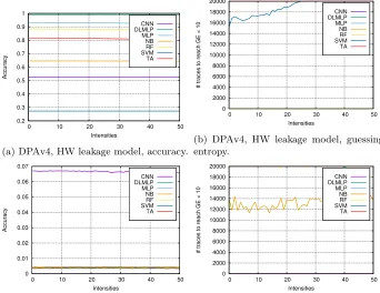
Next, we present and briefly discuss several characteristic scenarios for pub-licly available datasets. In Figure 4, we depict results for DPAv4 and AES RD datasets. First, in Figure 4a, we see how the accuracy is high, and for all classi-fiers, except SVM, this dataset should be easy to classify. Such observations are confirmed from guessing entropy results (Figure 4b), as, for most of the classi-fiers, an increase in the perturbation intensity does not bring any decrease in the attack performance. The exception is SVM, where we observe how the per-formance decreases and already for intensity equal to 25, 20 000 attack traces is not enough to break the target. Finally, TA cannot break the target regardless of the perturbation level.
For AES RD, we observe that most of the classifiers perform on the level of random guessing (Figure 4c) except CNN, which has significantly higher ac-curacy. As we know that CNNs are well-equipped to handle the random delay countermeasure due to their spatial invariance [5, 8], this result can serve as a strong indication that CNN should be able to break the target rather easily. This is confirmed in Figure 4d, where we observe CNN breaking the target easily, and no amount of added perturbation makes the attack harder. An interesting result appears for NB, as it also breaks the target (granted, with orders of magnitude more traces than CNN). We postulate this happens due to its generative nature and independence of features assumption.
In Figure 5, we depict results for AES HD and ASCAD. First, for AES HD and accuracy, observe how the accuracy has erratic behavior when adding per-turbation. This happens because AES HD is already very noisy dataset to start with, and then, any change in the noise level, brings unstable behavior as many predictions are equally likely. The behavior for guessing entropy shows that while accuracy can be affected (as each measurement is treated separately), the effect of cumulative probabilities stabilizes the results for guessing entropy. Still, sev-eral methods cannot break the target even without added noise, while NB is most stable (as a consequence of feature independence assumption, the noise has less effect).
Finally, we show results for the ASCAD dataset. From the accuracy perspec-tive, several methods can be considered as performing well, but still under the influence of added noise (RF, CNN, DLMLP). On the other hand, SVM conducts random guessing regardless of the added noise. Finally, NB, MLP, and TA classi-fiers show more oscillations in their behavior due to added noise. On the guessing entropy side, we observe that classifiers do not suffer much when adding more perturbation. CNN and DLMLP perform very well, while TA cannot break the implementation even with 20 000 traces and regardless of the perturbation level. Other classifiers perform reasonably well (similar as in related works), where RF has most problems with handling high perturbation levels.
0.2 0.3 0.4 0.5 0.6 0.7 0.8 0.9 1
0 10 20 30 40 50
Accuracy Intensities CNN DLMLP MLP NB RF SVM TA
(a) DPAv4, HW leakage model, accuracy. 0 2000 4000 6000 8000 10000 12000 14000 16000 18000 20000
0 10 20 30 40 50
# traces to reach GE < 10
Intensities CNN DLMLP MLP NB RF SVM TA
(b) DPAv4, HW leakage model, guessing entropy. 0 0.01 0.02 0.03 0.04 0.05 0.06 0.07
0 10 20 30 40 50
Accuracy Intensities CNN DLMLP MLP NB RF SVM TA
(c) AES RD, intermediate value leakage model, accuracy. 0 2000 4000 6000 8000 10000 12000 14000 16000 18000 20000
0 10 20 30 40 50
# traces to reach GE < 10
Intensities CNN DLMLP MLP NB RF SVM TA
(d) AES RD, intermediate value leakage model, guessing entropy.
Fig. 4: Results for the DPAv4 and AES HD datasets.
and indicate that we can model various effects with noise, but also, that our framework can be used in various settings.
6
General Observations and Remarks
There are four main types of behavior one can expect when modeling the system with perturbations. We give the list in the order from the most preferred to the least preferred setting:
1. “Resilient” behavior. In this setting, the classifier is resilient to perturba-tions, which means that its performance remains practically unchanged even in the presence of noise. Naturally, after some point, the performance starts to deteriorate, and then, the behavior resembles one of the following types. 2. “Stable” behavior. In this setting, the classifier is affected by perturbation,
and the performance is gradually decreased.
0.0032 0.0034 0.0036 0.0038 0.004 0.0042 0.0044 0.0046 0.0048 0.005
0 10 20 30 40 50
Accuracy Intensities CNN DLMLP MLP NB RF SVM TA
(a) AES HD, intermediate value leakage model, accuracy. 0 2000 4000 6000 8000 10000 12000 14000 16000 18000 20000
0 10 20 30 40 50
# traces to reach GE < 10
Intensities CNN DLMLP MLP NB RF SVM TA
(b) AES HD, HW leakage model, guessing entropy. 0.0034 0.0036 0.0038 0.004 0.0042 0.0044 0.0046 0.0048 0.005
0 10 20 30 40 50
Accuracy Intensities CNN DLMLP MLP NB RF SVM TA
(c) ASCAD, intermediate value leakage model, accuracy. 4000 6000 8000 10000 12000 14000 16000 18000 20000
0 10 20 30 40 50
# traces to reach GE < 10
Intensities CNN DLMLP MLP NB RF SVM TA
(d) ASCAD, HW leakage model, guessing entropy.
Fig. 5: Results for the AES HD and ASCAD datasets.
4. “No learning” behavior. With this behavior, the perturbation does not in-fluence the performance of the profiling method. This happens because the classifier, even before perturbation, was not working, and naturally, making the problem more difficult cannot improve the behavior but also cannot de-teriorate it. While this behavior has certain similarities with the first one, the underlying idea is different. Here, the classifier never works while in the “Resilient” setting, it is stable up to a certain level of perturbation (i.e., no difference between that level of perturbation and no perturbation).
Besides these four types, there are several subtypes one can recognize by combin-ing the traits of the basic behaviors. Next, we give several remarks that clarify the potential of our framework. Note that we give this in a classifier-agnostic way.
can be a very volatile concept that depends on many factors) into the most stable method.
2. If the dataset is easy to attack, adding perturbations does not significantly influence the performance. Indeed, our results indicate that the classifiers then behave as “Resilient” or “Stable”.
3. If the dataset is difficult to attack due to noise, then adding perturbation commonly results in “Unstable” behavior.
4. Accuracy is the least resilient metric for perturbations as we consider each measurement separately. More resilience to perturbation happens with guess-ing entropy and success rate due to the cumulative probabilities approach. Additionally, we observe an interesting trade-off. From the performance side without added perturbation, guessing entropy is more powerful as it consid-ers all key guesses and not only the best one. When adding perturbation, the success rate is more stable as it considers only the best guess, so it avoids any instability stemming from multiple key guesses that are (approximately) equally likely.
5. When considering the random delay and masking countermeasures, we see that the classifiers can work easier with random delay and perturbation than with masking and perturbation. This indicates that masking benefits more from added noise than random delay, which is especially interesting for portability settings where there are always differences between the profiling and attack device.
6. With our framework, it is possible to “map” different setting: for instance, 1) to see what level of perturbation causes the classifiers to behave in the same way as, e.g., having a masking countermeasure, or, 2) at what point the suboptimal hyperparameter results in the same behavior as an added perturbation.
Besides these observations, we make two more remarks:
– The generative nature of TA and NB gives those methods more resilience to perturbations, which is especially pronounced for NB, as there, we also work under feature independence assumption.
– Our results indicate that accuracy is not a reliable measure for the interme-diate value leakage model for difficult datasets. This is well-known for the Hamming weight model [7].
7
Conclusions
In this paper, we concentrate on the problem of profiled side-channel attacks and uncertainties stemming from the experimental results. To that end, we propose a general framework that can be used to analyze the behavior of any profiled side-channel attack (i.e., a method performing the classification task). Our framework supports datasets with any characteristics as well as different leakage models. To offer such a general behavior, we model it as the expectation estimation problem where we can achieve any desired accuracy and confidence level. After we model the classifiers, we use the robustness analysis to estimate their performance in the presence of perturbations. Such an analysis allows us to answer the question of which classifier is the best for some scenarios. We give robustness analysis for all standard figures of merit in SCA: accuracy, success rate, and guessing entropy.
We believe our framework to be a powerful tool that will allow researchers to compare the behavior of various classifiers in a more fair way than it is done up to now. Since profiled SCA in realistic settings should consider different pro-filing and attacking devices, we see that our framework allows us more than just connecting SCA with problems that have reliable theoretical results. More precisely, our framework allows modeling the realistic behavior of profiled SCA, where uncertainty must occur because of several different noise sources.
We note that our framework is demanding: to conduct a proper analysis, the Chernoff bound requires a large number of samples, which potentially can be a prohibiting factor for specific computationally intensive classifiers or very large datasets. One easy way how to circumvent this is to parallelize the process for different intensities. Another option, which we plan to explore in the future work is to use the Chernoff-Okamoto bound that is tighter than the Chernoff bound. Since it applies when p≤0.5 only, it remains to be seen how useful this bound can be in the SCA domain.
References
1. Mangard, S., Oswald, E., Popp, T.: Power Analysis Attacks: Revealing the Secrets
of Smart Cards. Springer (December 2006) ISBN 0-387-30857-1, http://www.
dpabook.org/.
2. Choudary, O., Kuhn, M.G.: Efficient template attacks. In Francillon, A., Rohatgi, P., eds.: Smart Card Research and Advanced Applications - 12th International Conference, CARDIS 2013, Berlin, Germany, November 27-29, 2013. Revised Se-lected Papers. Volume 8419 of LNCS., Springer (2013) 253–270
3. Chari, S., Rao, J.R., Rohatgi, P.: Template Attacks. In: CHES. Volume 2523 of LNCS., Springer (August 2002) 13–28 San Francisco Bay (Redwood City), USA. 4. Heuser, A., Zohner, M.: Intelligent Machine Homicide - Breaking Cryptographic
Devices Using Support Vector Machines. In Schindler, W., Huss, S.A., eds.:
COSADE. Volume 7275 of LNCS., Springer (2012) 249–264
-19th International Conference, Taipei, Taiwan, September 25-28, 2017, Proceed-ings. (2017) 45–68
6. Picek, S., Heuser, A., Jovic, A., Ludwig, S.A., Guilley, S., Jakobovic, D., Mentens, N.: Side-channel analysis and machine learning: A practical perspective. In: 2017 International Joint Conference on Neural Networks, IJCNN 2017, Anchorage, AK, USA, May 14-19, 2017. (2017) 4095–4102
7. Picek, S., Heuser, A., Jovic, A., Bhasin, S., Regazzoni, F.: The curse of class im-balance and conflicting metrics with machine learning for side-channel evaluations.
IACR Transactions on Cryptographic Hardware and Embedded Systems2019(1)
(Nov. 2018) 209–237
8. Kim, J., Picek, S., Heuser, A., Bhasin, S., Hanjalic, A.: Make some noise. unleashing the power of convolutional neural networks for profiled side-channel analysis. IACR
Trans. Cryptogr. Hardw. Embed. Syst.2019(3) (2019) 148–179
9. Zaid, G., Bossuet, L., Habrard, A., Venelli, A.: Methodology for efficient cnn
architectures in profiling attacks. IACR Transactions on Cryptographic Hardware
and Embedded Systems2020(1) (Nov. 2019) 1–36
10. Bhasin, S., Chattopadhyay, A., Heuser, A., Jap, D., Picek, S., Shrivastwa, R.R.: Mind the portability: A warriors guide through realistic profiled side-channel
anal-ysis. Cryptology ePrint Archive, Report 2019/661 (2019)https://eprint.iacr.
org/2019/661.
11. Valiant, L.: Probably Approximately Correct: Nature’s Algorithms for Learning and Prospering in a Complex World. Basic Books, Inc., New York, NY, USA (2013)
12. Kocher, P.C.: Timing Attacks on Implementations of Diffie-Hellman, RSA, DSS,
and Other Systems. In: Proceedings of CRYPTO’96. Volume 1109 of LNCS.,
Springer-Verlag (1996) 104–113
13. Kocher, P.C., Jaffe, J., Jun, B.: Differential power analysis. In: Proceedings of the 19th Annual International Cryptology Conference on Advances in Cryptology. CRYPTO ’99, London, UK, UK, Springer-Verlag (1999) 388–397
14. Quisquater, J.J., Samyde, D.: Electromagnetic analysis (ema): Measures and
counter-measures for smart cards. In Attali, I., Jensen, T., eds.: Smart Card
Programming and Security, Berlin, Heidelberg, Springer Berlin Heidelberg (2001) 200–210
15. Genkin, D., Shamir, A., Tromer, E.: Acoustic cryptanalysis. Journal of Cryptology
30(2) (Apr 2017) 392–443
16. Schindler, W., Lemke, K., Paar, C.: A Stochastic Model for Differential Side
Channel Cryptanalysis. In LNCS, ed.: CHES. Volume 3659 of LNCS., Springer (Sept 2005) 30–46 Edinburgh, Scotland, UK.
17. Heuser, A., Rioul, O., Guilley, S.: Good is Not Good Enough — Deriving Optimal Distinguishers from Communication Theory. In Batina, L., Robshaw, M., eds.: CHES. Volume 8731 of Lecture Notes in Computer Science., Springer (2014) 18. Lerman, L., Poussier, R., Bontempi, G., Markowitch, O., Standaert, F.:
Tem-plate attacks vs. machine learning revisited (and the curse of dimensionality in side-channel analysis). In Mangard, S., Poschmann, A.Y., eds.: Constructive Side-Channel Analysis and Secure Design - 6th International Workshop, COSADE 2015, Berlin, Germany, April 13-14, 2015. Revised Selected Papers. Volume 9064 of Lec-ture Notes in Computer Science., Springer (2015) 20–33
19. Hospodar, G., Gierlichs, B., De Mulder, E., Verbauwhede, I., Vandewalle, J.: Ma-chine learning in side-channel analysis: a first study. Journal of Cryptographic
20. Lerman, L., Bontempi, G., Markowitch, O.: Power analysis attack: An approach based on machine learning. Int. J. Appl. Cryptol.3(2) (June 2014) 97–115 21. Lerman, L., Bontempi, G., Markowitch, O.: A machine learning approach against
a masked AES - Reaching the limit of side-channel attacks with a learning model.
J. Cryptographic Engineering5(2) (2015) 123–139
22. Lerman, L., Medeiros, S.F., Bontempi, G., Markowitch, O.: A Machine Learn-ing Approach Against a Masked AES. In: CARDIS. Lecture Notes in Computer Science, Springer (November 2013) Berlin, Germany.
23. Picek, S., Heuser, A., Guilley, S.: Template attack versus Bayes classifier. Journal
of Cryptographic Engineering7(4) (Nov 2017) 343–351
24. Gilmore, R., Hanley, N., O’Neill, M.: Neural network based attack on a masked implementation of AES. In: 2015 IEEE International Symposium on Hardware Oriented Security and Trust (HOST). (May 2015) 106–111
25. Heuser, A., Picek, S., Guilley, S., Mentens, N.: Lightweight ciphers and their
side-channel resilience. IEEE Transactions on ComputersPP(99) (2017) 1–1
26. Maghrebi, H., Portigliatti, T., Prouff, E.: Breaking cryptographic implementations using deep learning techniques. In: Security, Privacy, and Applied Cryptography Engineering - 6th International Conference, SPACE 2016, Hyderabad, India, De-cember 14-18, 2016, Proceedings. (2016) 3–26
27. van der Valk, D., Picek, S., Bhasin, S.: Kilroy was here: The first step towards
explainability of neural networks in profiled side-channel analysis. Cryptology
ePrint Archive, Report 2019/1477 (2019)https://eprint.iacr.org/2019/1477.
28. van der Valk, D., Picek, S.: Bias-variance decomposition in machine
learning-based side-channel analysis. Cryptology ePrint Archive, Report 2019/570 (2019)
https://eprint.iacr.org/2019/570.
29. Masure, L., Dumas, C., Prouff, E.: Gradient visualization for general characteri-zation in profiling attacks. In Polian, I., St¨ottinger, M., eds.: Constructive Side-Channel Analysis and Secure Design - 10th International Workshop, COSADE 2019, Darmstadt, Germany, April 3-5, 2019, Proceedings. Volume 11421 of Lec-ture Notes in Computer Science., Springer (2019) 145–167
30. Picek, S., Heuser, A., Guilley, S.: Profiling side-channel analysis in the restricted
attacker framework. Cryptology ePrint Archive, Report 2019/168 (2019) https:
//eprint.iacr.org/2019/168.
31. Alippi, C.: Intelligence for Embedded Systems: A Methodological Approach.
Springer Publishing Company, Incorporated (2014)
32. Rudin, W.: Real and Complex Analysis, 3rd Ed. McGraw-Hill, Inc., New York, NY, USA (1987)
33. Chernoff, H.: A measure of asymptotic efficiency for tests of a hypothesis based
on the sum of observations. Ann. Math. Statist.23(4) (12 1952) 493–507
34. Hoeffding, W.: Probability inequalities for sums of bounded random variables. Journal of the American Statistical Association58(301) (1963) 13–30
35. TELECOM ParisTech SEN research group: DPA Contest (4thedition) (2013–2014)
http://www.DPAcontest.org/v4/.
36. Coron, J., Kizhvatov, I.: An Efficient Method for Random Delay Generation in Embedded Software. In: Cryptographic Hardware and Embedded Systems - CHES 2009, 11th International Workshop, Lausanne, Switzerland, September 6-9, 2009, Proceedings. (2009) 156–170
37. Prouff, E., Strullu, R., Benadjila, R., Cagli, E., Dumas, C.: Study of deep learning techniques for side-channel analysis and introduction to ASCAD database. IACR
38. Regazzoni, F., Cevrero, A., Standaert, F.X., Badel, S., Kluter, T., Brisk, P., Leblebici, Y., Ienne, P.: A design flow and evaluation framework for DPA-resistant instruction set extensions. In Clavier, C., Gaj, K., eds.: CHES09. Volume 5747 of LNCS. Springer (September 2009) 205–19
39. Standaert, F.X., Malkin, T.G., Yung, M.: A unified framework for the analysis of sidechannel key recovery attacks. In Joux, A., ed.: Advances in Cryptology -EUROCRYPT 2009, Berlin, Heidelberg, Springer Berlin Heidelberg (2009) 443– 461
40. Fern´andez-Delgado, M., Cernadas, E., Barro, S., Amorim, D.: Do we Need
Hun-dreds of Classifiers to Solve Real World Classification Problems? Journal of
Ma-chine Learning Research15(2014) 3133–3181
41. Friedman, N., Geiger, D., Goldszmidt, M.: Bayesian Network Classifiers. Machine
Learning29(2) (1997) 131–163
42. Fan, R.E., Chen, P.H., Lin, C.J.: Working Set Selection Using Second Order
Infor-mation for Training Support Vector Machines. J. Mach. Learn. Res.6(December
2005) 1889–1918
43. Breiman, L.: Random Forests. Machine Learning45(1) (2001) 5–32
44. Goodfellow, I., Bengio, Y., Courville, A.: Deep Learning. MIT Press (2016)http: //www.deeplearningbook.org.
45. James, G., Witten, D., Hastie, T., Tibsihrani, R.: An Introduction to Statistical Learning. Springer Texts in Statistics. Springer New York Heidelbert Dordrecht London (2001)
A
Influence of Hyperparameter Change
We evaluate the attack performance with changed hyperparameters to examine the behavior of our framework when using suboptimal profiling methods. More precisely, we select the second-best performing hyperparameter combinations for several classifiers. Here, we use SVM with C = 0.001 and γ = 0.001, RF with 100 trees, and MLP with feature selection and ReLU activation function, adam solver, and (50,30,50) configuration of layers/nodes. Figures 6a and 6b show results for ASCAD with guessing entropy, and DPAv4 with success rate, respectively. For ASCAD, we see that changed hyperparameters only slightly decreased performance, but now, adding noise makes the results much less stable. For DPAv4, we depict results for success rate, and we observe stable behavior in the presence of added noise. The success rate can be less influenced by added noise than guessing entropy since it uses cumulative probabilities (which adds stability) but does not consider less likely guesses (where added noise more easily causes miss-classification).
B
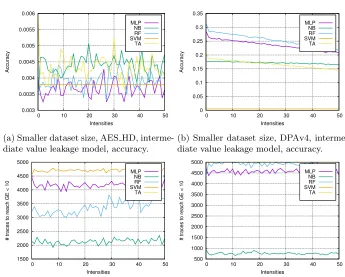
Influence of the Dataset Size Change
13000 14000 15000 16000 17000 18000 19000 20000
0 10 20 30 40 50
# traces to reach GE < 10
Intensities MLP
RF SVM
(a) Suboptimal hyperparameters for AS-CAD, HW leakage model, guessing en-tropy.
0 5 10 15 20 25 30 35
0 10 20 30 40 50
Success Rate
Intensities
MLP RF SVM
(b) Suboptimal hyperparameters for
DPAv4, HW leakage model, success rate.
Fig. 6: Changes in hyperparameters.
0.003 0.0035 0.004 0.0045 0.005 0.0055 0.006
0 10 20 30 40 50
Accuracy
Intensities MLP
NB RF SVM TA
(a) Smaller dataset size, AES HD, interme-diate value leakage model, accuracy.
0 0.05 0.1 0.15 0.2 0.25 0.3 0.35
0 10 20 30 40 50
Accuracy
Intensities MLP
NB RF SVM TA
(b) Smaller dataset size, DPAv4, interme-diate value leakage model, accuracy.
1500 2000 2500 3000 3500 4000 4500 5000
0 10 20 30 40 50
# traces to reach GE < 10
Intensities MLP
NB RF SVM TA
(c) Smaller dataset size, ASCAD, HW leak-age model, guessing entropy.
500 1000 1500 2000 2500 3000 3500 4000 4500 5000
0 10 20 30 40 50
# traces to reach GE < 10
Intensities MLP
NB RF SVM TA
(d) Smaller dataset size, AES HD, HW leakage model, guessing entropy.