Multiphoton amplitude in a constant background field
Aftab Ahmad1,2,, Naser Ahmadiniaz3,, Olindo Corradini4,5,, Sang Pyo Kim3,6,, and ChristianSchubert2,†
1Department of Physics, Gomal University, 29220 D.I. Khan, K.P.K., Pakistan.
2Instituto de Física y Matemáticas, Universidad Michoacana de San Nicolás de Hidalgo. Edificio C-3, Ciudad Universitaria, Morelia 58040, Michoacán, México.
3Center for Relativistic Laser Science, Institute for Basic Science, Gwangju 61005, Korea.
4Dipartimento di Scienze Fisiche, Informatiche e Matematiche, Universitá di Modena e Reggio Emilia, Via Campi 213/A, I-41125 Modena, Italy.
5INFN, Sezione di Bologna, Via Irnerio 46, I-40126 Bologna, Italy.
6Department of Physics, Kunsan National University, Kunsan 54150, Korea.
Abstract.In this contribution, we present our recent compact master formulas for the multiphoton amplitudes of a scalar propagator in a constant background field using the worldline fomulation of quantum field theory. The constant field has been included non-perturbatively, which is crucial for strong external fields. A possible application is the scattering of photons by electrons in a strong magnetic field, a process that has been a subject of great interest since the discovery of astrophysical objects like radio pulsars, which provide evidence that magnetic fields of the order of 1012G are present in
na-ture. The presence of a strong external field leads to a strong deviation from the classical scattering amplitudes. We explicitly work out the Compton scattering amplitude in a magnetic field, which is a process of potential relevance for astrophysics. Our final result is compact and suitable for numerical integration.
1 Introduction
The “worldline” or “Feynman-Schwinger” [1] representation of the one-loop effective action in scalar
QED is
Γ[A] = −
∞
0
dT T e−m
2T
PDx(τ) e
−0Tdτ[14x˙2+iex˙µAµ(x(τ))]. (1)
HeremandT denote the mass and proper-time of the loop scalar, andPDx(τ) the path integral over closed loops in (Euclidean) spacetime with periodicityT in the proper-time. The above path integral
e-mail: aftab.gu@gmail.com
e-mail: ahmadiniaz@ibs.re.kr (speaker)
e-mail: olindo.corradini@unimore.it
e-mail: sangkim@kunsan.ac.kr
can be converted into the following master formula for the N-photon (off-shell) amplitudes [2, 3]
Γ(k1, ε1;. . .;kN, εN) = −(−ie)N(2π)DδD
N
i=1
ki ∞
0
dT T (4πT)−
D
2e−m2T
N
i=1
T
0 dτi
×exp N
i,j=1
1
2GBi jki·kj−iGBi jεi˙ ·kj+ 1
2GBi jεi¨ ·εjε1ε2···εN. (2)
HereGBi j, ˙GBi jand ¨GBi jare the “bosonic” worldline Green’s function and its first and second deriva-tives with respect to the first variable (GBi j≡GB(τi−τj) etc):
GBi j=|τi−τj| −(τi−τj)
2
T , GBi j˙ =sign(τi−τj)−2 τi−τj
T , GBi j¨ =2δ(τi−τj)− 2
T . (3) GBi jis the Green’s function for the operator d2
dτ2 with the periodic boundary condition, also obeying the “string-inspired” (SI) boundary conditions: 0TdτiGBi j =0TdτjGBi j =0. The notationε1ε2···εN means taking linear terms in each polarization vector after expanding the exponential. This master formula is extremely compact and well-organized with respect to gauge invariance [2–4]. See [3] for its generalization to the spinor QED case, [6, 7] for multi-loop generalizations, and [5] for a review on the worldline formalism. For scalar QED in the presence of a constant background fieldFµν, a similar “Bern-Kosower type” master formula was obtained in [8, 9]:
Γ(k1, ε1;. . .;kN, εN) = −(−ie)N(2π)DδD
N
i=1
ki ∞
0
dT T (4πT)−
D
2e−m2Tdet−12 sin(Z)
Z
×
N
i=1
T
0 dτiexp
N
i,j=1
1
2ki· GBi j·kj−iεi·G˙Bi j·kj+ 1
2εi·G¨Bi j·εjε1ε2···εN, (4)
whereZ =eFT. The main differences between this master formula and the vacuum one in Eq. (2)
is the additional factor det−1sinZ Z
, and the replacement of theGBi jGreen’s function with a new one GBi jthat is a function of the external field:
GBi j=T 2Z2
Z
sin(Z)e−iZ
˙
GBi j+iZGBi j˙ −1. (5)
This Green’s function also follows the SI boundary conditions. This master formula, and particularly its extension to spinor QED [5, 10], are generally more efficient for constant field calculations in QED
than the standard method based on Feynman diagrams. They have already been applied to photonic processes in a constant field like vacuum polarization [5, 10, 11], photon splitting (in a magnetic field) [5, 12] and the two loop Euler-Heisenberg Lagrangian [5, 9]. Much less has been done for the corresponding amplitudes with an open line (propagator) instead of the closed loop, either in vacuum or in an external field. In 1996 Daikouji et al. [13] obtained the following “Bern-Kosower type” master formula for the N-photon dressed scalar propagator in vacuum (see also [14] for a recent rederivation):
Dpp
(k1, ε1;· · ·;kN, εN) = (−ie)N(2π)DδD
p+p+
N
i=1
ki ∞
0 dTe
−m2T
×
N
i=1
T
0 dτie
−T[p+1
TNi=1(kiτi−iεi)]2+Ni,j=1[∆i jki·kj−2i•∆i jεi·kj−•∆•i jεi·εj]
can be converted into the following master formula for the N-photon (off-shell) amplitudes [2, 3]
Γ(k1, ε1;. . .;kN, εN) = −(−ie)N(2π)DδD
N
i=1
ki ∞
0
dT T (4πT)−
D
2e−m2T
N
i=1
T
0 dτi
×exp N
i,j=1
1
2GBi jki·kj−iGBi jεi˙ ·kj+ 1
2GBi jεi¨ ·εjε1ε2···εN. (2)
HereGBi j, ˙GBi jand ¨GBi jare the “bosonic” worldline Green’s function and its first and second deriva-tives with respect to the first variable (GBi j≡GB(τi−τj) etc):
GBi j=|τi−τj| −(τi−τj)
2
T , GBi j˙ =sign(τi−τj)−2 τi−τj
T , GBi j¨ =2δ(τi−τj)− 2
T . (3) GBi jis the Green’s function for the operator d2
dτ2 with the periodic boundary condition, also obeying the “string-inspired” (SI) boundary conditions: 0TdτiGBi j =0TdτjGBi j =0. The notationε1ε2···εN means taking linear terms in each polarization vector after expanding the exponential. This master formula is extremely compact and well-organized with respect to gauge invariance [2–4]. See [3] for its generalization to the spinor QED case, [6, 7] for multi-loop generalizations, and [5] for a review on the worldline formalism. For scalar QED in the presence of a constant background fieldFµν, a similar “Bern-Kosower type” master formula was obtained in [8, 9]:
Γ(k1, ε1;. . .;kN, εN) = −(−ie)N(2π)DδD
N
i=1
ki ∞
0
dT T (4πT)−
D
2e−m2Tdet−12 sin(Z)
Z
×
N
i=1
T
0 dτiexp
N
i,j=1
1
2ki· GBi j·kj−iεi·G˙Bi j·kj+ 1
2εi·G¨Bi j·εjε1ε2···εN, (4)
whereZ=eFT. The main differences between this master formula and the vacuum one in Eq. (2)
is the additional factor det−1sinZ Z
, and the replacement of theGBi jGreen’s function with a new one GBi jthat is a function of the external field:
GBi j= T 2Z2
Z
sin(Z)e−iZ
˙
GBi j+iZGBi j˙ −1. (5)
This Green’s function also follows the SI boundary conditions. This master formula, and particularly its extension to spinor QED [5, 10], are generally more efficient for constant field calculations in QED
than the standard method based on Feynman diagrams. They have already been applied to photonic processes in a constant field like vacuum polarization [5, 10, 11], photon splitting (in a magnetic field) [5, 12] and the two loop Euler-Heisenberg Lagrangian [5, 9]. Much less has been done for the corresponding amplitudes with an open line (propagator) instead of the closed loop, either in vacuum or in an external field. In 1996 Daikouji et al. [13] obtained the following “Bern-Kosower type” master formula for the N-photon dressed scalar propagator in vacuum (see also [14] for a recent rederivation):
Dpp
(k1, ε1;· · ·;kN, εN) = (−ie)N(2π)DδD
p+p+
N
i=1
ki ∞
0 dTe
−m2T
×
N
i=1
T
0 dτie
−T[p+1
TiN=1(kiτi−iεi)]2+iN,j=1[∆i jki·kj−2i•∆i jεi·kj−•∆•i jεi·εj]
ε1ε2···εN, (6)
where∆i jis the open line Green’s function adopted to Dirichlet boundary conditions (DBC)
∆(τi, τj)=τiτj
T +
|τi−τj|
2 −
τi+τj
2 , ∆(0, τj)= ∆(T, τj)= ∆(τi,0)= ∆(τi,T)=0. (7) For this Green’s function, we need to distinguish between derivatives with respect to first and second
k3
+ −p p
k2 k1 k3 kN
· · ·
+ −p p
k2 k1 k3 kN
· · · −p p
k1 k2 k3 kN
· · ·
−p p
k1 k2 kN
· · ·
... ...
+ +
+ +
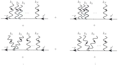
Figure 1.Multi-photon Compton-scattering diagram.
argument, since the DBC break the translation invariance in proper-time. A convenient notation is [15] to use left and right dots to indicate derivatives with respect to the first and the second argument, respectively:
•∆
i j = τj T +
1
2sign(τi−τj)− 1
2 , •∆•i j= 1
T −δ(τi−τj),
∆•i j = τi
T − 1
2sign(τi−τj)− 1
2 , 2∆i j=GBi j−GBi0−GB0j, (8) where the last formula gives a relation between∆i jandGBi j[16]. The organization of the paper is as follows. In section 2 we include the constant field into the Green’s function of a scalar propagator, then dress it with N photons to obtain master formulas in configuration and momentum space. In section 3 we work the momentum space formula out forN = 2 to find a compact representation
of the Compton scattering cross section in a general constant field. In section 4 we summarize our discussion.
2 Scalar propagator in a constant field
In the previous section we have presented a master formula for an open line in vacuum, in the follow-ing we consider a constant external field to be included in this master formula. We first start with a free propagator in a constant field.
2.1 Free propagator
A constant field in the Fock-Schwinger gauge is written as
Aµ(y)=−1
2Fµν(y−x)ν , A(y=x)=0 (xis the reference point of the potential). (9) After decomposing the arbitrary trajectoryx(τ) into a straight-line part and a fluctuation part
x(τ)=x+ τ
and using (9) andQµ=T
0 dτqµ(τ), with some manipulations the free scalar propagator can be written
as
Dxx
[A] =
∞
0 dTe
−m2T x(T)=x
x(0)=x Dxe
−0Tdτ14x˙2+iex˙·A(x)
=
∞
0 dTe
−m2T−(x−x)2 4T
Dq(τ) e−0Tdτ14q
−d2
dτ2+2ieF
d dτ
q+ie
T(x−x)FQ, (11)
which is gaussian. Now besides the free path integral normalization Dq(τ)e−0Tdτq
−1 4d
2
dτ2
q
=
4πT−D
2 [5] we have to take into account the ratio of the field-dependent and free path integral nor-malization:
Det−12
P
−14 d
2
dτ2 +12ieFddτ
Det−12
P
−14 d
2
dτ2
=Det−
1 2
P
1−2ieF d dτ
−1=det−1 2sin(Z)
Z
, (12)
where we have eliminated the zero mode which exists in the path integral by putting a ‘prime’. Now we have to introduce a new Green’s function which is again related to the one with SI boundary conditions in (5) for a constant field:
∆
i j≡ τi|
d2
dτ2 −2ieF
d dτ
−1
|τjDBC=12GBi j− GBi0− GB0j+GB00. (13)
After using this Green’s function in the usual completing-the-square procedure, we get the following well-known representation of the scalar propagator in a constant external field inx-space:
Dxx
(F) =
∞
0 dTe
−m2T e−(x−x)2
4T (4πT)−D2det−12
sin(eFT)
eFT
e0Tdτ
T
0 dτieT(x−x)F∆(τ,τ )ie
TF(x−x)
=
∞
0 dTe
−m2T
(4πT)−D
2det12
Z sinZ
e−1
4T(x−x)ZcotZ(x−x). (14)
After Fourier transforming its representation in momentum space gives
Dpp
(F)=(2π)Dδ(p+p)D(p,F) , D(p,F)= ∞
0 dTe
−m2T e−T p( tanZ
Z )p
det12[cosZ]
. (15)
2.2 Dressed propagator
Now, if we dress the scalar propagator with N photons in addition to the constant field, we write the potential asA=Aext+Aphotwhich the former is the same as in (9) and the later is written as a sum of
plane waves, each photon is represented as a vertex operator:
Aµ
phot=
N
i=1
εµieiki·x , VA[k, ε]=
T
0 dτε·x˙(τ) e
ik·x(τ) = T 0 dτe
ik·x(τ)+ε·x˙(τ)
lin(ε). (16)
The path integral representation of the scalar propagator in a constant field dressed with N photons is written as
Dxx
(F|k1, ε1;· · ·;kN, εN)=(−ie)N
∞
0 dTe
−m2T
PDxe
and using (9) andQµ=T
0 dτqµ(τ), with some manipulations the free scalar propagator can be written
as
Dxx
[A] =
∞
0 dTe
−m2T x(T)=x
x(0)=x Dxe
−0Tdτ14x˙2+iex˙·A(x)
=
∞
0 dTe
−m2T−(x−x)2 4T
Dq(τ) e−0Tdτ14q
−d2
dτ2+2ieF
d dτ
q+ie
T(x−x)FQ, (11)
which is gaussian. Now besides the free path integral normalization Dq(τ)e−0Tdτq
−1 4d
2
dτ2
q
=
4πT−D
2 [5] we have to take into account the ratio of the field-dependent and free path integral nor-malization:
Det−12
P
−14 d
2
dτ2 +12ieFddτ
Det−12
P
−14 d
2
dτ2
=Det−
1 2
P
1−2ieFd dτ
−1=det−1 2sin(Z)
Z
, (12)
where we have eliminated the zero mode which exists in the path integral by putting a ‘prime’. Now we have to introduce a new Green’s function which is again related to the one with SI boundary conditions in (5) for a constant field:
∆
i j≡ τi|
d2
dτ2 −2ieF
d dτ
−1
|τjDBC= 12GBi j− GBi0− GB0j+GB00. (13)
After using this Green’s function in the usual completing-the-square procedure, we get the following well-known representation of the scalar propagator in a constant external field inx-space:
Dxx
(F) =
∞
0 dTe
−m2T e−(x−x)2
4T (4πT)−D2det−12
sin(eFT)
eFT
e0Tdτ
T
0 dτieT(x−x)F∆(τ,τ )ie
TF(x−x)
=
∞
0 dTe
−m2T
(4πT)−D
2det12
Z sinZ
e−1
4T(x−x)ZcotZ(x−x). (14)
After Fourier transforming its representation in momentum space gives
Dpp
(F)=(2π)Dδ(p+p)D(p,F) , D(p,F)= ∞
0 dTe
−m2T e−T p( tanZ
Z )p
det12[cosZ]
. (15)
2.2 Dressed propagator
Now, if we dress the scalar propagator with N photons in addition to the constant field, we write the potential asA=Aext+Aphotwhich the former is the same as in (9) and the later is written as a sum of
plane waves, each photon is represented as a vertex operator:
Aµ
phot=
N
i=1
εµieiki·x , VA[k, ε]=
T
0 dτε·x˙(τ) e
ik·x(τ)= T 0 dτe
ik·x(τ)+ε·x˙(τ)
lin(ε). (16)
The path integral representation of the scalar propagator in a constant field dressed with N photons is written as
Dxx
(F|k1, ε1;· · ·;kN, εN)=(−ie)N
∞
0 dTe
−m2T
PDxe
−0Tdτ[14x˙2+iex˙·Aext(x)]VA[k1, ε1]· · ·VA[kN, εN]. (17)
After applying the path decomposition (10) and completing the square we get (x−=x−x)
Dxx
(F|k1, ε1;· · ·;kN, εN) = (−ie)N
∞
0 dTe
−m2T (4πT)−D
2det12 Z sinZ
e−1
4Tx−ZcotZx−
× T
0 dτ1· · ·
T
0 dτNe N
i=1
εi·xT−+iki·x−
τi
T +iki·x
×exp N
i,j=1
ki∆
i jkj−2iεi •∆
i jkj−εi •∆
•
i jεj
+2e
T x− N
i=1
F◦∆ iki−iF
◦∆ •
iεi
ε1ε2···εN, (18)
where a left (right) ‘open circle’ on∆
(τ, τ
) denotes an integralT
0 dτ(
T
0 dτ). Thisx-space master
formula was obtained by McKeon and Sherry for a purely magnetic field [17]. Now we can Fourier transform to momentum space to get
Dpp
(F|k1, ε1;· · · ;kN, εN) = (−ie)N(2π)Dδ
p+p+
N
i=1
ki ∞
0 dTe
−m2T 1 det12[cosZ]
× T
0 dτ1· · ·
T
0 dτNe N
i,j=1ki∆
i jkj−2iεi •∆
i jkj−εi •∆
•
i jεje−Tb(tanZ Z )b
ε1ε2···εN,
b ≡ p+ 1
T N
i=1
τi−2ieF◦∆ i
ki−i1−2ieF◦∆ • i εi . (19)
Diagrammatically, these master formula hold the full information on the set of Feynman diagrams appearing in Fig. 1, with the full scalar propagator in a constant field (usually indicated by a double line).
3 Compton scattering in a constant field
Now, let us apply our momentum space master formula in (19) to work out the Compton scattering cross section, corresponding toN = 2. Notice that our master formula describes theuntruncated
dressed propagator so in applying it to physical processes one has to truncate the external scalars, we define the matrix elementT as
T(F|k1, ε1;· · ·;kN, εN)= D
pp
(F|k1, ε1;· · ·;kN, εN)
D(p,F)D(p,F) . (20) Moreover, it will be convenient to Wick rotate from Euclidean to Minkowski space (see [18] for our conventions). Expanding out the exponentials in (19) up to terms linear in both polarizations we arrive at
Dpp
(F|k1, ε1;k2, ε2) = e2
∞
0 dT
e−m2T det12[cosZ]
T
0 dτ1dτ2e
−Tb0(tanZZ)b0+2i,j=1ki∆
i jkjε1M12ε2, (21)
with
b0 ≡ p+T1 2
i=1
τi−2ieF◦∆ i
ki,
M12 ≡ 2•∆•12−T2
1+2ie◦∆
•T 1F tanZ Z
1−2ieF◦∆ •
2
+4(1+2ie◦∆
•T
1F)tanZZb0− 2
i=1
•∆ 1iki
b0tanZ
Z
1−2ieF◦∆ •
2− 2 i=1 ki∆ •
To obtain the cross section we square and sum over the photon polarizations viapolε∗iµενi → gµν which finally leads to the following expression for the Compton cross section:
pol
T∗T = e4
|D(p,F)2|D(p,F)2
∞
0 dT
e−m
2T
det12[cosZ] T
0 dτ
1
T
0 dτ
2e−
Tb∗
0(tanZZ)b∗0+2i,j=1ki∆
i jkj
× ∞
0 dT
e−m2T det12[cosZ]
T
0 dτ1
T
0 dτ2e
−Tb0(tanZZ)b0+2i,j=1ki∆
i jkjtr(M†
12M12). (23)
4 Summary
In this short report we have extended our previous master formulas for multiphoton amplitudes in vacuum in scalar QED [14] to include a constant external field using the worldline formalism, see [18] for more details. Our master formula is valid off-shell, and combines the various orderings of
the N photons along the scalar line. We have worked out the cross section for the case ofN = 2,
that is linear Compton scattering in the field, reaching a compact integral representation suitable for numerical evaluation. This cross section is, for the magnetic field case, of importance for astrophysics, but appears to have been studied so far only in the strong-field limit [19].
References
[1] R.P. Feynman, Phys. Rev.80, 440 (1950).
[2] Z. Bern and D. A. Kosower, Phys. Rev. Lett.66, 1669 (1991); Nucl. Phys.B 379, 451 (1992). [3] M. J. Strassler, Nucl. Phys.B 385, 145 (1992).
[4] N. Ahmadiniaz, C. Schubert and V.M. Villanueva, JHEP1301(2013) 312. [5] C. Schubert, Phys. Rept.355, 73 (2001).
[6] M. G. Schmidt and C. Schubert, Phys. Lett. B33169 (1994), hep-th/9403158.
[7] M.G. Schmidt and C. Schubert, Phys. Rev. D 53, 2150 (1996), hep-th/9410100.
[8] R. Zh. Shaisultanov, Phys. Lett.B 378, 354 (1996).
[9] M. Reuter, M. G. Schmidt and C. Schubert, Ann. Phys. (N.Y.)259, 313 (1997). [10] C. Schubert, Nucl. Phys.B 585, 407 (2000).
[11] W. Dittrich and R. Shaisultanov, Phys. Rev.D 62, 045024 (2000). [12] S.L. Adler and C. Schubert, Phys. Rev. Lett.77.
[13] K. Daikouji, M. Shino, Y. Sumino, Phys. Rev.D 53, 4598 (1996).
[14] N. Ahmadiniaz, A. Bashir and C. Schubert, Phys. Rev.D 93, 045023 (2016). [15] F. Bastianelli and P. van Nieuwenhuizen, Cambridge University press, 2006. [16] D. Fliegner, M.G. Schmidt and C. Schubert, Z. Phys.C 64, 111 (1994). [17] D.G.C. McKeon and T.N. Sherry, Mod. Phys. Lett.A9, 2167 (1994).