Pushing the Boundaries in Gradient and Shim Design for MRI

(1)

Scholarship@Western

Electronic Thesis and Dissertation Repository

3-4-2011 12:00 AM

Pushing the Boundaries in Gradient and Shim Design for MRI

Parisa Hudson

The University of Western Ontario

Supervisor

Dr. Blaine Chronik

The University of Western Ontario Graduate Program in Physics

A thesis submitted in partial fulfillment of the requirements for the degree in Doctor of Philosophy

Follow this and additional works at: https://ir.lib.uwo.ca/etd

Part of the Physics Commons, and the Sustainability Commons

Recommended Citation Recommended Citation

Hudson, Parisa, "Pushing the Boundaries in Gradient and Shim Design for MRI" (2011). Electronic Thesis and Dissertation Repository. 99.

https://ir.lib.uwo.ca/etd/99

This Dissertation/Thesis is brought to you for free and open access by Scholarship@Western. It has been accepted for inclusion in Electronic Thesis and Dissertation Repository by an authorized administrator of

(2)

(Spine title: Design of high performance gradient and shim coils)

(Thesis format: Integrated- Article)

by

Parisa Hudson

Graduate Program in Physics and Environment and sustainability

A thesis submitted in partial fulfillment of the requirements for the degree of

Doctor of Philosophy

The School of Graduate and Postdoctoral Studies The University of Western Ontario

London, Ontario, Canada

(3)

ii

THE UNIVERSITY OF WESTERN ONTARIO School of Graduate and Postdoctoral Studies

CERTIFICATE OF EXAMINATION

Supervisor

______________________________ Dr. Blaine A. Chronik

Supervisory Committee

______________________________ Dr. David S. Rosner

______________________________ Dr. Tamie L. Poepping

______________________________ Dr. Robert Lannigan

Examiners

______________________________ Dr. Michael D. Noseworthy

______________________________ Dr. Eugene Wong

______________________________ Dr. Paul A. Wiegert

______________________________ Dr. Charles A. McKenzie

The thesis by

Parisa Hudson

entitled:

Pushing the boundaries in gradient and shim design for MRI

is accepted in partial fulfillment of the requirements for the degree of

Doctor of Philosophy

______________________ _______________________________

(4)

iii

Abstract

High performance gradient and shim coils are highly interested for high-field magnetic resonance imaging and spectroscopy to correct for large B0 inhomogeneities created by the

magnetic susceptibility differences between tissues, bone, and air. In chapter two, complete sets of high-performance gradient and shim coils are designed using two different methods: the minimum inductance and the minimum power target field methods. A quantitative comparison of shim performance in terms of merit of inductance, ML, and merit of resistance, MR, is made for shim coils designed using the minimum inductance and the minimum power design algorithms. The coils designed using the target field method are not controlled over the length of the coil. In order to produce realistic coils for use in human or small-animal studies, direct control over the length of the coils is necessary. Therefore in chapter three, an extended Fourier series method for the design of shim coils with

predetermined length is presented. This simple method is based on a truncated Fourier series expansion of the current density to allow for explicit control over the coil length. This method is mathematically simple, easy to implement and computationally fast. Also a quantitative comparison of figures of merit for inductance and resistance is made as a

function of shim coil length. Coils of 40 cm diameter are designed with lengths of 50 cm, 60 cm, 80 cm, and 100 cm.

(5)

iv

(6)

v

Co-Authorship Statement

(7)

vi

Acknowledgments

I express my appreciation to all those who have helped me academically and personally throughout this research. I express many thanks and appreciation to my supervisor, Blaine Chronik, for his guidance and insight throughout the completion of this Ph.D. project. Blaine has always given me valuable suggestions and comments to make this project successful.

Special thanks to William Handler who has been like a second supervisor to me. Will has been a great mentor and a wonderful adviser during this project. His assistance and

knowledge has been invaluable to me during this work. Mr. Handler, I will never forget your kindness and support over the past five years.

I have been fortunate to work with wonderful colleges and friends over the course of this project. Many thanks to Tim Scholl, Jamu Alford, Chad Harris, Kyle Gilbert, Dustin Haw and Rebecca Feldman. It has been a great pleasure to work with such wonderful friends.

I would like to show my gratitude to Joe Gati and Martyn Klassen for providing the field maps and anatomical images for this project.

(8)

vii

List of Tables

Table 2.1 Performance values for ten shim axes designed using minimum inductance and minimum power algorithms. In every design case, the improvement in ML provided by the minimum inductance method is less than 10% of the value obtained using the minimum power method and the improvements in MR provided by the minimum power method are less than 15% of the values obtained using the minimum inductance method. The merit of

inductance calculated with the discrete method agrees with the merit of inductance calculated with the continuous method within 3.5% in all cases. The difference between the merits of power calculated with the discrete and the continuous methods ranges between 10% and 30%. ... 47

Table 3.1 Inductive merit, ML, values for all 28 distinct shim axis pairs designed using minimum inductance and minimum power algorithms. The differences in ML between the minimum inductance and minimum power designs were less than 6% in all cases. Across most shim axes, the 80 cm length designs had the highest inductive merit values. ... 66

Table 3.2 Resistive merit, MR, values for all 28 distinct shim axis pairs designed using minimum inductance and minimum power algorithms. The differences in MR between the minimum inductance and minimum power designs were less than 6% in all cases. Across all shim axes, the 80 cm length designs had the highest resistive merit values... 66

(12)

xi

List of Figures

Figure 1.1 A recent transverse in vivo T2-weighted MR image of a normal human wrist

acquired by Uchiyama et al. is shown in a) and the first transverse MR image of a normal human wrist acquired by Hinshaw et al. is shown in b). ... 2

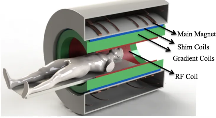
Figure 1.2 Schematic of an MRI scanner is shown with cut-away section including the

principle components. ... 4

Figure 1.3 FID signals received from a) a well-shimmed sample and b) a poorly-shimmed sample. ... 8

Figure 1.4 An example of z-shimming by Yang et al. (29) shows axial gradient-echo images of brain. a) The first image is acquired with no compensation. b) The second image is

acquired with a 20% slice refocusing gradient area offset and the third image is acquired with a 40% of slice refocusing gradient area offset, and (d) shows the sum of images (a), (b), and (c) which is an artifact free image. ... 10

Figure 1.5 Non-oblique-sliced DSU homogeneity improvement for selected slices in a 32-slice acquisition, a) shows the field maps acquired using static global FASTMAP and b) the field maps acquired using second-order dynamic shimming updating... 11

Figure 1.6 Residual magnetic field maps near auditory air cavities of a mouse are presented using a) no shim, b) a one-material (zirconium) passive shim and c) a two- material passive shim... 12

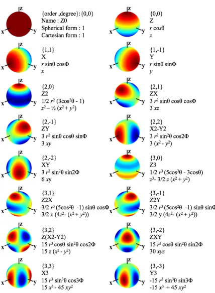
Figure 1.7 Plots of the spherical harmonics are shown up to 3rd order on the surface of a sphere. The equations for the spherical harmonics are given in spherical (r, θ, φ) and

Cartesian (x, y, z) coordinates. ... 14

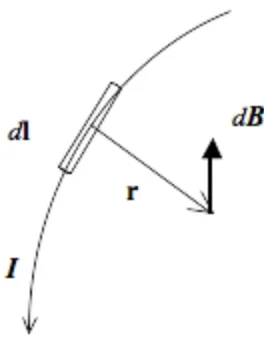
Figure 1.8 The elemental form of Biot-Savart law is shown with Idl as the source of magnetic field and dB as the resulting field. ... 16

(13)

xii

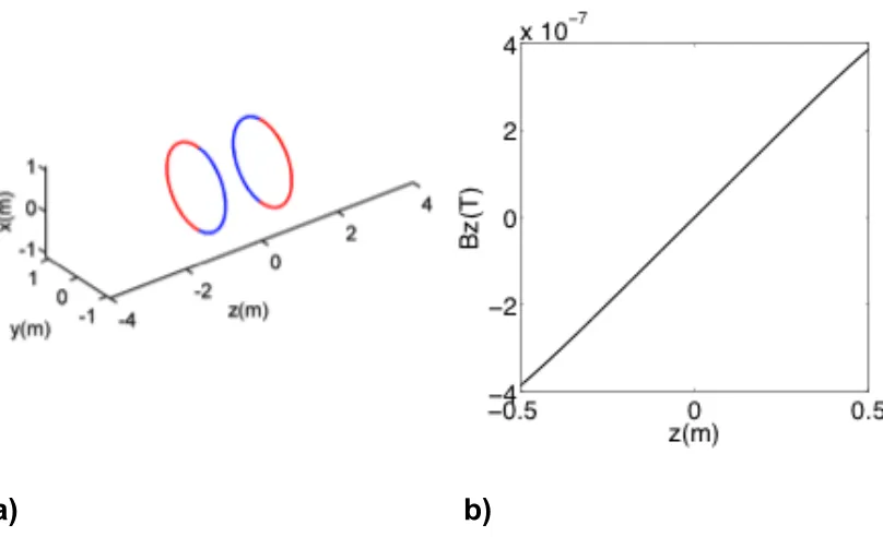
radius of the loop. b) The z-component of the magnetic field is plotted as function of z

within the region of interest... 18

Figure 1.10 a) An arrangement of a Maxwell coil is shown with two loops of wire separated by a distance √3a and anti-parallel currents. b) the z-component of the magnetic field is plotted as function of z within the region of interest. ... 19

Figure 1.11 a) An arrangement of a Y coil is shown with coil spacing for optimal gradient uniformity. b) The z-component of the magnetic field is plotted as function of z within the region of interest... 20

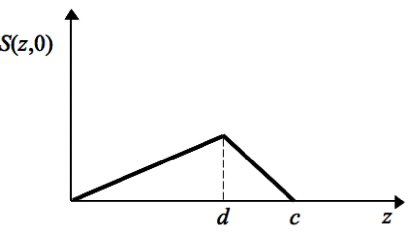
Figure 1.12 A plot of the stream function S(z,0), for φ= 0, for a transverse gradient coil is

shown. The arcs position is then determined by finding the equally spaced contours of the stream function. The wire pattern of the coil is shown figure 1.13. ... 23

Figure 1.13 The wire pattern of a transverse gradient coil resulting by the stream function given by Eq. [1.21] is shown... 24

Figure 2.1 The upper half (z > 0) of the Z2 wire pattern given by (a) minimum inductance and (b) minimum power methods. The bottom halves of the coils are mirror images of the top halves not shown in this figure. Minimum power designs tend to feature longer, less

compact wire patterns than minimum inductance designs... 38

Figure 2.2 The upper half (z > 0) of the X2–Y2 wire pattern given by (a) minimum inductance and (b) minimum power methods. The bottom halves of the coils are mirror images of the top halves not shown in this figure. Minimum inductance designs tend to give more complex wire and more compact wire patterns than minimum power designs... 40

Figure 2.3 a) Magnetic field profile for Z2, normalized to the edge of the region of interest, on the z-axis (solid line). (b) Calculated magnetic field profile in the x and y directions for the X2_–Y2_{shim coil with a radius of}_a_{= 0.1 m. For the Z}2_{coil, the field targets (circles) were}

(14)

xiii

Figure 2.4 One quadrant of the relative residual fields (top figures) and the absolute residual fields (bottom figures) in the xy plane for the X2–Y2 shim coils designed using minimum inductance (a, c) and minimum power methods (b, d). Within the ROI and in the xy plane, the average relative residual fields are <2% and the average absolute residual fields are <10-7 T when evaluated using both design methods. The magnetic fields produced by the coils designed using minimum power and minimum inductance methods were scaled to have the same efficiency (17 mT/ m2/A)... 43

Figure 2.5 One quadrant of the relative residual fields (top figures) and the absolute residual fields (bottom figures) in the yz plane for the X2–Y2 shim coils designed using minimum inductance (a, c) and minimum power methods (b, d). Within the ROI and in the yz plane, the average relative residual fields are <4% and the average absolute residual fields are <10-6

T when evaluated using both design methods. The magnetic fields produced by the coils designed using minimum power and minimum inductance methods were scaled to have the same efficiency (17 mT/ m2/A). ... 44

Figure 3.1 Half-wire-patterns for ten coils: X, Y, Z, XY, X2-Y2, YZ, XZ, Z2, Z3, and Z4 at four different lengths given by minimum inductance and minimum resistance methods. All coils are symmetric about the cuts chosen. The minimum resistance designs tend to feature less oscillation with less number of loops than minimum inductance designs at the same coil length... 61

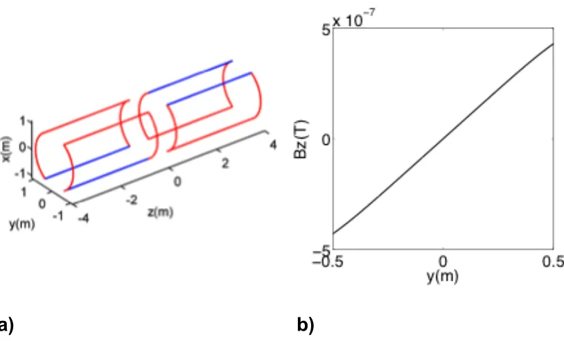
Figure 3.2 The z-component of the magnetic field profile in the z-y plane (x = 0) for a Z2 shim coil with a radius of a = 0.2 m. The region shown is larger than the originally specified region of interest, and it can be seen that the quadratic behavior of the magnetic field

continues well outside the region of interest... 62

Figure 3.3 The z-component of the magnetic field profile in the x-y plane (z = 0) for an XY shim coil with a radius of a = 0.2 m. ... 63

(15)

xiv

and yz planes are less than 5% for both formulations, indicating that both produced

comparable field uniformity... 64

Figure 4.1 A schematic view of a custom coil with a diameter of 40 cm and the length of 30 cm is shown. The coil’s region of interest has dimensions of 8 cm × 5 cm × 4 cm and is off centered. ... 73

Figure 4.2 A cylindrical surface mesh with 8300 elements, with a diameter of 40 cm, and a length of 30 cm was created using Comsol Multiphysics (Burlington, MA). ... 75

Figure 4.3 parts a), d) and g) show sagittal anatomical images and parts b), e) and h) show sagittal images of the unshimmed field inhomogeneity maps of all three subject heads

respectively. The field map of each subject head was overlaid with the anatomical image and the results are shown in parts c), f), and i). For each subject the white rectangle, shown in parts c), f), and i) encompasses the hippocampi... 78

Figure 4.4 The wire pattern of the coil is shown with 1 mm diameter wire and 60 windings. The inductance of the coil was calculated to be 960 µH and the resistance of the coil was 1.65

Ω. ... 79

Figure 4.5 The z-component of the magnetic field is shown along x, y and z-axes, within the region of interest... 80

Figure 4.6 Planar slices of the field inhomogeneity through the centre of the region of interest when a) no shims, b) simulated custom shim and the existing system shims were used. The simulated custom shim reduces the field inhomogeneity by a factor of 1.3 when added to the system shims as compared to that obtained using the shim system only... 81

Figure 4.7 Parts a), b), and c) show the simulated histograms of the frequency

(16)

xv

Figure 4.8 The standard deviation of residual frequency inhomogeneities after shimmed with the simulated custom plus system shims was calculated for many misalignments of one subject’s head within the custom coil. This figure shows that the misalignment of up to ± 1 cm could be tolerated in x-, y- and z- directions... 83

(17)

xvi

List of Appendices

Appendix A ... 50

(18)

xvii

List of Abbreviations and Symbols

MRI magnetic resonance imaging

MRS magnetic Resonance spectroscopy

RF radio frequency

SNR signal to noise ratio

FID free induction decay

FASTMAP fast automatic shimming technique by mapping along

projections

RASTAMAP robust automated shimming technique using

arbitrary mapping acquisition parameters

FOV field of view

DSU dynamic shimming updating

BEM boundary element method

ROI region of interest

RMS root mean squared

DC direct current

fMRI functional MRI

PCA principle component analysis

T2 spin-spin relaxation time

(19)

xviii

TR repetition time

MR merit of resistance

ML merit of inductance

η efficiency

L inductance

R resistance

P power

M torque

G gradient

B magnetic field

J current density

S stream function

U optimization functional for current

σ standard deviation

(20)

Chapter 1

1 Introduction

1.1 A Brief History of Magnetic Resonance Imaging

Magnetic Resonance Imaging has proven to be a powerful imaging technique for the visualization of internal structure of the body. It has the ability to create contrast between different soft tissues of the body, it possesses sensitivity to a broad range of tissue properties, and it allows for the early diagnosis of many diseases, in particular neurological, musculoskeletal, and cardiovascular diseases, and cancer.

Although several scientists like Larmor (1857-1942) (1), Isaac Rabi (1930's), Bloch and Purcell (1952) (2,3), and Damadian (1970’s) (4) introduced some basic steps towards the development of magnetic resonance imaging, first in vivo cross-sectional magnetic resonance images of a finger were acquired by Mansfield and Maudsley (5) in 1973. In the late 1970's and early 1980's a number of groups of scientists and

manufacturers showed promising results of MRI in vivo. The first commercial MR scanner in Europe (from Picker Ltd.) was installed in 1983 in the Department of Diagnostic Radiology at the University of Manchester Medical School (Professor I Isherwood & Professor B Pullen). Since then there has been an explosion of technology and science in the field and we have moved from crude noisy images to highly

sophisticated measurements. Figure 1.1 shows a) a recent transverse in vivo T2-weighted

(21)

A modern MRI scanner is capable of providing exquisite anatomical detail as well as functional information in perfusion and diffusion studies of the brain. Two- and three-dimensional MR angiography provide a roadmap of vessels in any part of the body, together with the ability to obtain functional velocity profiling of blood flow. This non-invasive imaging modality with a virtually limitless future is continuing today to make further major advances in diagnosing diseases.

a)

b)

Figure 1.1 A recent transverse in vivo T2-weighted MR image of a normal human wrist

acquired by Uchiyama et al. is shown in a) and the first transverse MR image of a normal human wrist acquired by Hinshaw et al. is shown in b).

1.1.1 The MRI Scanner

(22)

Permanent magnets are constructed with ferromagnetic materials and do not require electricity to run. However, these magnets are limited to low magnetic field strength. Super-conducting magnets (9) are most commonly used clinically and are composed of super-conducting material, such as Niobium-Titanium (Nb3Ti). The super-conducting windings are immersed in liquid helium to reduce the temperature of the alloy to a level that makes them superconductive.

Shim coils (10) are located within the magnet bore and create magnetic fields in a variety of shapes to compensate for the field inhomogeneities in the magnetic field and make the field more uniform for imaging (This process is further explained in detail in this chapter). Shim coils may be super-conducting and/or room-temperature resistive coils of wire.

Gradient coils (10) are usually located inside the shim coils and are designed to produce linear magnetic field gradients in the imaging region, which collectively and sequentially are superimposed on the main magnetic field, B0, for the selective spatial

excitation of the imaging volume. There are typically three sets of gradient coils creating three orthogonal field gradients in the x-, y- and z-directions in conventional MRI

coordinates. The gradient in the z-direction, Gz, is conventionally used in the slice selecting process. This gradient is defined as a slice select gradient that causes a linear variation in the resonant frequency in z-direction across the sample. When a slice is selected by irradiating the sample with an RF pulse, in the presence Gz, only a slice of finite thickness, Δz, is excited. The gradient in the x-direction, Gx, is conventionally used in the frequency encoding process. This gradient is perpendicular to the slice select gradient. This gradient applies a field gradient and causes a linear variation in the resonant frequency in x-direction in order to encode the x-position of the sample. The third gradient, Gy, is conventionally used in the phase encoding process. This gradient, which is perpendicular to Gx and Gz, is turned on before the frequency encoding gradient

to encode the y-position via the phase of the signal.

(23)

electromagnetic field that excites the protons at their resonant frequency, and also detects the signal generated by the precessing spins after excitation. During the excitation, the slice thickness is determined by the spectral bandwidth of the RF pulse along with the strength of the gradient field. RF coils can be divided into three general categories: transmit and receive coils, receive only coils, and transmit only coils. Transmit and receive coils serve as the transmitter of the RF field and receiver of signals from the imaged object. A transmit only coil is used to create the magnetic field and a receive only coil is used in conjunction with the transmit coil to detect or receive signals from the imaged object.

Figure 1.2 Schematic of an MRI scanner is shown with cut-away section including the principle components.

1.2 Magnetic Field Inhomogeneities

The demand for making more powerful magnets to generate stronger magnetic fields is increasing. With increasing magnetic field strength, the signal to noise ratio (SNR) increases in MRI. This increase in field strength is accompanied by many

(24)

average value of the field is known as field inhomogeneities. The inhomogeneities of the static main magnetic field are caused by two major sources: the imperfect magnet and the magnetic environment, and the susceptibility of the imaging object.

1.2.1 Imperfect Magnet and Magnetic Environment

In practice it is not possible to build a perfect magnet. Imperfections in the main magnet design and construction create field inhomogeneities that should be addressed. Ferromagnetic objects in the vicinity of the magnet, the metal impurities in gradient systems and magnet shielding around the scanner room also contributes to the creation of the field inhomogeneities. These field inhomogeneities are usually on the order of 100 parts per million (ppm) and are often corrected by placing magnetic materials close to the area that experiences large field inhomogeneities and allowing the field to be shimmed.

1.2.2 Susceptibility-Induced Magnetic Field Inhomogeneities

The imaging objects such as a human subject, an animal or a device perturb the magnetic field due to their susceptibilities when placed in an MRI scanner. Such

susceptibility induced field inhomogeneities have been simulated by several authors (11-13) and the field inhomogeneities have been shown to be sharper and stronger at

boundaries between materials with different susceptibilities. The strength of the field inhomogeneities scales with the strength of the magnetic field. Thus at higher magnetic field, the field inhomogeneities generated at the interface of tissues of different magnetic susceptibilities are higher (14,15). These field inhomogeneities are usually a few parts per million (ppm).

The field inhomogeneities generated by the imperfect magnet and susceptibility of an imaging object are known as static field inhomogeneities, and cause signal loss and therefore image distortion. An image is distorted due to field inhomogeneities created in two directions: distortion due to field inhomogeneities in the slice selection direction, G′z

(25)

1.2.3 Field Inhomogeneities in the Slice Select Direction

The effect of field inhomogeneities in the slice select direction, G′z on the signal

are found by looking at phase behavior. The equation for a signal received from a region of a sample at a time t (10) could be written as:

!

S(t)"

%

#

( )

r ei$( )t dxdydz (1.1)

where ρ(r) is the spin density and φ(t) is the phase that could be written as:

!

"(t)=#

(

G(r)$r

)

t. (1.2)

G(r) is the field gradient. Without the effect of the field inhomogeneities:

!

G r

_{( )}

=Gxi+Gyj+Gzk. (1.3)

During the slice select process, the equation for signal is:

!

S( t )" #

( )

r eiGzztdz

$

(1.4)

The presence of the field inhomogeneities in the slice select direction, G′z, can cause misregistration of the signal as a function of slice location since the measured signal is now affected by G′z:

!

S( t )" #

( )

r ei G( z+G $z)zt

dz

%

(1.5)

The addition of G′z, to Gz can also lead to a slice thickness different from the

designed value because the slice thickness is inversely proportional to Gz + G′z.

1.2.4 Field Inhomogeneities in the Plane of the Slice

(26)

select process could cause the excited plane to be rotated (10). During the phase encoding process this could cause slice distortion resulting in positional misregistration of the signal.

1.3 Correcting the Field, Shimming

Magnetic field inhomogeneities can be reduced using ferroshims and shim coils. Ferroshims are pieces of ferromagnetic materials placed in the bore of the magnet or areas that suffer from large field inhomogeneities so as to correct the inhomogeneities. This process is described in detail in section 1.3.4. Shim coils are resistive coils of wire carrying currents controlled by the user to minimize the field inhomogeneities. In section 1.4, various techniques that have been developed to design high performance shim coils are described. Several methods have been developed to reduce the field inhomogeneities by either using the ferroshims or shim coils.

1.3.1 FID Shimming

One way to correct for the field inhomogeneities is free induction decay

shimming. The free induction decay signal coming from a sample is affected by the field

inhomogeneities through the signal decay time,

!

T₂"_{. The increase in the field}

inhomogeneities, decreases

!

T₂"_{and therefore causes the FID signal to decay more}

(27)

a)

b)

Figure 1.3 FID signals received from a) a well-shimmed sample and b) a poorly-shimmed sample.

1.3.2 Field Map-Based Shimming

This method of shimming relies on the measurement of the field inhomogeneities that need to be shimmed. In this method, a 3D field generated by each shim coil is measured for a phantom at the center of the shim coils and a matrix describing all the shim fields, Bshim_{is created (21). The optimal shim currents vector,}_I_{, is obtained by}

multiplying the pseudo inverse, †, of Bshim_{with a vector of field values,}_b_{, required to}

null the field inhomogeneities at each spatial position throughout the sample:

!

I =

(

Bshim

)

+b. (1.6)

(28)

lines to give enough information for the determination of shim currents. However this method incorrectly assumes that shim coil fields are always fully characterized by a minimal set of spherical harmonics. Later, robust automated shimming technique using arbitrary mapping acquisition parameters (RASTAMAP) (28) was developed by using a fast, accurate, and flexible pulse sequence that can compensate for phase errors and generate absolute field maps regardless of the field of view (FOV) resolution, and acquisition geometry, making it ideally suited for automated shimming applications. In this method the shim fields are fitted to the field inhomogeneity map using linear least squares fitting in order to find the optimum current in each shim coil.

1.3.3 z

-Shimming

The presence of the field inhomogeneities in the slice select direction, G′z could be eliminated by z-shimming (29). As mentioned in section 1.2.3, the gradient field in the slice direction could be separated into two terms; Gzand G′z, where Gz is the gradient field generated by the slice select gradient and G′z is the field inhomogeneities in the slice select direction. The effect of G′z could be removed by applying a compensation gradient offset, Gc in time duration tc such that:

!

"

G _zt#Gctc=0 (1.7)

To perform the z-shimming technique, a normal image (figure 1.4a) with Gc = 0 is acquired. This image shows large signal loss in the inferior frontal cortex and inferior lateral temporal regions. Two subsequent images (figures. 1.4b and 1.4c) were acquired with increasing compensation gradient, Gctc. Figures 1.4b and 1.4c show the

enhancement in the signal only in regions where the field inhomogeneities are

(29)

Figure 1.4 An example of z-shimming by Yang et al. (29) shows axial gradient-echo images of brain. a) The first image is acquired with no compensation. b) The second image is acquired with a 20% slice refocusing gradient area offset and the third image is acquired with a 40% of slice refocusing gradient area offset, and (d) shows the sum of images (a), (b), and (c) which is an artifact free image.

1.3.4 Dynamic Shimming

Similar to field-map-based shimming, dynamic shimming updating (DSU) uses the linear least squares fitting to fit the shim fields with the field inhomogeneity map in order to find the optimum currents in shim coils. However in dynamic shimming the fitting is performed separately for each slice during a multi-slice imaging acquisition that allows for optimal local modeling and updating of shim currents for separate slices. This method of shimming removes the locally manageable field inhomogeneities in a global fashion. Figure 1.5 shows the field maps of brain for selected slices in a 32-slice acquisition after a) static global FASTMAP optimized shimming and b) second order dynamic shimming. As shown in the field maps, dynamic shimming significantly reduces the field inhomogeneities in frontal lobe as compared to FASTMAP shimming (30). The current in the shim coils needs to be switched rapidly during dynamic

(30)

magnetic field that is generated during switching currents in the shim coils) the shim coils may be actively shielded.

a)

b)

Figure 1.5 Non-oblique-sliced DSU homogeneity improvement for selected slices in a 32-slice acquisition, a) shows the field maps acquired using static global FASTMAP and b) the field maps acquired using second-order dynamic shimming updating.

1.3.5 Local Passive Shimming

(31)

Similarly, Koch et al. (32) have shown that a prototype shim comprised of both diamagnetic (bismuth) and paramagnetic (zirconium) materials improve the field inhomogeneities significantly in a mouse brain. Figure 1.6 shows an example of the residual field maps when a) no shimming, b) one material passive shimming and c) two- material passive shimming were performed.

Figure 1.6 Residual magnetic field maps near auditory air cavities of a mouse are presented using a) no shim, b) a one-material (zirconium) passive shim and c) a two- material passive shim.

1.4 Spherical Harmonic

In regions of space with free sources of current density, J, the Maxell equations that govern the magnetic field are simplified to (36):

!

" #B = 0 (1.8)

!

" #B = 0 (1.9)

Using the vector identity

!

" # " #B =" " $

(

B

)

-"2B, Eqs. [1.8] and [1.9], Laplace’s

(32)

!

"2B = 0. (1.10)

If only the z-component of the magnetic field is considered, Laplace’s equation could be simplified to:

!

"2Bz = 0. (1.11)

The general solution of Laplace’s equation in spherical coordinates is a linear combination of spherical harmonic functions (36):

!

B_z

_{( )}

r = C_nm

m=-n

n

"

n=0

#

"

rn_P n

m _cos

$

(

)

eim%

(1.12)

where Pnm are Legendre polynomials with positive integer order n and positive integer degree m≤n. Cnm is the amount of the nth order, mth degree spherical harmonic present in Bz(r). Figure 1.7 shows all the 0th_{, 1}st_{, 2}nd_{and 3}rd_{order spherical harmonic functions}

(33)

(34)

Since the magnetic field vector can be described by spherical harmonic functions, the deviation from homogeneities can also be expressed on that basis. Active shimming capitalizes on this principle by using a set of shim coils, each generating one component of magnetic field that correspond to one spherical harmonic. These coils minimize the magnetic field inhomogeneities by superimposing a shim field with the same special distribution and magnitude but opposite sign to inhomogeneities.

1.5 Designing Shim and Gradient Coils

With a serious need for better quality gradient and shim coils, various methods have been developed to design these current-carrying coils of wire to generate magnetic field whose axial component is in shape of a spherical harmonic. These methods are categorized under the discrete windings method and the distributed windings method.

1.5.1 Biot Savart Law

One of the most fundamental equations used in coil design is the Biot-Savart law. Using this equation, the elemental magnetic field dB(r) generated by a current I,through a wire element of length dl could be written as (37):

!

dB = µ0Idl"r

4#r3 (1.13)

where r is the distance between the point at which the magnetic field is calculated and the wire element and r is the magnitude of vector r as shown in figure 1.8. The total

(35)

Figure 1.8 The elemental form of Biot-Savart law is shown with Idl as the source of magnetic field and dB as the resulting field.

1.5.2 Coil Performance

The performance of a coil depends on the application for which it is used. This includes the efficiency of the coil, the field uniformity, the inductance, the resistance, the torque, and the figure of merits.

The efficiency,η, of a coil is defined as the amount of spherical harmonic

magnetic field generated by the coil per unit current and has the unit of Tm-nA-1, where n is the order of the spherical harmonic generated by the coil. The accuracy with which the desired magnetic field is generated by the coil could be defined as the field uniformity. To characterize the field uniformity, the relative field residual defined as the percent difference between the actual field and the assumed ideal shape of the field in the region of interest could be calculated.

(36)

coil, and the amount of the torque that coil experiences in an intense static magnetic field respectively.

Inductive and resistive merits suggested by Turner (38) are used for comparing the performance of the gradient and shim coils. These two quantities defined such that they are independent of the number of turns of wire used in the coil.

The inductive merit is defined as:

!

ML= "

L (1.14)

and resistive merit for a rectangular wire is defined as:

!

MR= "

R. (1.15)

1.5.3 Coils with Discrete Windings

(37)

and their z-positions to dictate the degree, m, of the harmonics and annuls lower and some higher remaining unwanted harmonics.

1.5.3.1 Zonal Coils: Helmholtz and Maxwell Coils

Helmholtz and Maxwell coils are designed by only keeping the zonal spherical harmonic (those with no φdependence, m = 0) expansion (39) of the magnetic field. A

Helmholtz coil with m = 0 and n = 0 consists of two coaxial circular loops separated by a distance a, equal to the radius of loops. This coil generates a uniform magnetic field at center of the coil and is used to operate as Z0 shim coil within the MRI systems. Using this coil, a magnetic field with deviation of up to 5% is obtained within a sphere of radius 0.5a. Figure 1.9 shows a) the Helmholtz coil arrangement and b) the z-component of the magnetic field as function of z, within the region of interest.

a)

b)

(38)

A Maxwell coil with m = 0 and n =1, also consists of two circular loops but with the loop separation of √3 a, and currents flowing in reverse directions in the loops (39), such that a magnetic field varying linearly with z is produced. This coil could be

operated as a Z gradient coil within an MRI system. Similar to a Helmholtz coil, this coil also generates a magnetic field with deviation of up to 5% within a sphere of radius 0.5a. An arrangement of a Maxwell coil is shown in figure 1.10a and the z-component of the magnetic field as a function of z within the region of interest is shown in 1.10b.

a)

b)

Figure 1.10 a) An arrangement of a Maxwell coil is shown with two loops of wire separated by a distance √3a and anti-parallel currents. b) the z-component of the magnetic field is plotted as function of z within the region of interest.

1.5.3.2 Tesseral Coils: Golay Coil

(39)

placing 120o circular arcs of current with opposite sense at appropriate z positions. The z component of the magnetic field as function of y is shown in b).

a)

b)

Figure 1.11 a) An arrangement of a Y coil is shown with coil spacing for optimal gradient uniformity. b) The z-component of the magnetic field is plotted as function of z within the region of interest.

In order to achieve high magnetic field intensity, many loops of wire should be used with the discrete design and using many number of loops forces the loops to be positioned farther from the correct location and therefore introduces field errors. Furthermore the inductance of such coils is higher, since the loops are close together.

1.5.4 Coils with Distributed Windings

(40)

stream function methods, target field methods, the Fourier series method and the boundary element methods.

1.5.4.1 Matrix Inversion Methods

This method relies on the expansion of the magnetic field to find the optimal current flowing on surface of the coil. In 1997 Holt (41) suggested that the axial component of the magnetic field generated by a coil could be written as:

!

B_z= A_mn n=1

N

"

I_n (1.16)

where:

!

A_mn= µ0a2 2

(

z_m"zn

)

2

+a2 #

$

% & _'(

3

2 (1.17)

is a matrix that relates the axial component of the field at point zm on the axis to the current In flowing in the nth circular loop located at a position zn of a solenoid of radius a. To find a set of currents at N positions, the matrix Amn is inverted. The major weakness of this method is that the field could be specified in such a way the matrix becomes singular. Further improvements were made by Compton (42) who introduced a

predetermined error by departing the magnetic field created by the coil from the desired field. In this method, the surface of the coil was divided into 2048 equally sized

elementary areas and similar to Holt’s approach the axial component of the magnetic field at position k can be written:

!

B_zk = A_kj

j=1 n

"

I_j (1.18)

where Akj is a matrix for which each entry is the coefficient of the magnetic field at the point a resulting from a current Ij at a differential surface element j. By subtracting this

field from desired field,

!

(41)

!

E_k =Bzk 0

"Bzk =Bzk

0 _- _A

kj j=1

n

#

I_j (1.19)

and minimizing

!

E_k2

k=1

vol

"

with respect to the current elements Ij, a set of n simultaneous

equations is derived that could be solved by a matrix inversion method to find the surface current elements Ij. The wire pattern can be found by integrating over the elements of surface area until the current required for the coil in a discrete wire is accumulated. The transverse and longitudinal gradient coils designed using this method, create optimal field uniformity over the volume of the interest. However this method is computationally slow since a 2048 × 2048 matrix is inverted. Furthermore inductance or power is not

constrained in this method.

1.5.4.2 Stream Function Method

The continuity equation for the current density, ∇. J = 0, allows the current density to be described as the curl of a scalar function, the stream function, S(z, φ):

!

J =" #S) e r (1.20)

Various gradient coils with distributed windings have been designed by

considering simple stream functions capable of generating gradient fields of the desired symmetry. In this method the stream function is used to represent a current flow. Since a special change in the value of the stream function corresponds to an equivalent change in the current density, the contour plots of S(z, φ) gives the locations of the discrete wire

(42)

!

S z,

( )

" = I0z

d cos" z <d

= I0

(

c#z

)

c#d

(

)

cos" d < z <c = 0 elsewhere

(1.21)

where I0 is the total current flowing in the coil, c and d are the parameters that could be

adjusted to allow for some degree of optimization. For example, considering large values for c and d, results in a linear transverse gradient field over a large volume. Figure 1.12 shows the plot of the stream function for φ= 0 for Edelstein-type transverse gradient coil.

(43)

Figure 1.13 The wire pattern of a transverse gradient coil resulting by the stream function given by Eq. [1.21] is shown.

Coils designed with the stream function method generally have a good efficiency, but the gradient homogeneity tends to be poor.

1.5.4.3 Target Field Methods

Turner developed the powerful target field method (44) that uses the expansion of the Green’s function,

!

G r,

₍

r "

₎

= 1 r# "r

, for the Laplacian, in cylindrical coordinates to

(44)

fields and the inductance. This functional was then minimized to give the optimal current density. The complete mathematical derivation for the target field method is presented in chapter two where the minimum inductance design is compared with the minimum power design for a set of gradient and shim coils.

1.5.4.4 Fourier Series Method: Finite Length Coil Design

The length of cylindrical or planar coils designed with the target field method is unbounded and could not be controlled. Chronik and Rutt (45) modified the target field method by constraining the extent of the current density. This method is computationally slow since a large number of current constraints are used to force the current density to remain contained within a finite length. For the design of gradient coils with finite length, Carlson et al (46) developed a Fourier series method. In their method, the current density is expanded as a sum of odd sinusoidal functions for the Z gradient coil:

!

j_"m _#,z

( )

=$ # %

(

a

)

&_nsin n'z l (

)

* +

,

- z

n=%N N

.

/l

j_"m _#,z

( )

=0 z>l

(1.22)

and a sum of even sinusoidal functions for transverse gradient coils (X or Y coil):

!

j_"m

#,z

( )

=$ # %

(

a

)

&ncos

n'z

l

(

)

* +

,

- z

n=%N N

.

/l

j_"m

#,z

( )

=0 z >l

(1.23)

In Eqs. [1.22] and [1.23], a is the radius of the coil, l is the length of the coil and λn are the unknown coefficients. Using a functional that includes the magnetic field,

inductance, power or both, the optimal current density can be derived via λn while

(45)

1.5.4.5 The Boundary Element Method

This method is capable of designing gradient and shim coils wound on an arbitrary surface. This method, which was first developed by Pissanetzky (47), relies on discretization of the current density into elements on a mesh. A functional was made of the magnetic field, the inductance and the torque and minimized to allow for finding the optimal discretized current density while minimizing the inductance and the torque. Further Pool and Bowtell (48) modified this method by adding a power term to the functional to also minimize the power dissipation in the coil. In chapter four, the complete derivation of the boundary element method for the design of region specific custom shim coils is presented.

1.6 Scope of This Thesis

In chapter two, the minimum inductance and minimum power target field methods are described, and the mathematical derivations for both are presented. A quantitative comparison of minimum inductance and the minimum power algorithms is made for the design of shim coils for small animal imaging.

As previously mentioned, Carlson et al. developed a Fourier series method to design gradient coils with finite length. In chapter three, the technique of Carlson is extended to design shim coils with finite length by introducing a general 3D Fourier series of the current density. Also a quantitative comparison of shim coils performance at four lengths: 50 cm, 60 cm, 80 cm, and 100 cm designed using minimum power and minimum inductance algorithms is made.

(46)

1.7 References or Bibliography

1. Tubridy N, McKinstry CS. Neuroradiological history: Sir Joseph Larmor and the basis of MRI physics. Neuroradiology 2000;42(11):852-855.

2. Purcell EM, Torrey HC, Pouond RV. Resonance absorption by nuclear magnetic moments in a solid. Phys Rev 1946;69:37–38.

3. Bloch F. The Principle of Nuclear Induction. Science 1953;118(3068):425-430.

4. Kjelle MM. Raymond Damadian and the Development of MRI (Unlocking the Secrets of Science): Mitchell Lane Publishers; 2002. 48 pages p.

5. Mansfield P, Maudsley AA. Medical Imaging by NMR. Br J Radiol 1977;50(592):188– 194.

6. Uchiyama S, Itsubo T, Yasutomi T, Nakagawa H, Kamimura M, Kato H. Quantitative MRI of the wrist and nerve conduction studies in patients with idiopathic carpal tunnel syndrome. J Neurol Neurosurg Psychiatry 2005;76(8):1103-1108.

7. Hinshaw WS, Bottomley PA, Holland GN. Radiographic thin-section image of the human wrist by nuclear magnetic resonance. Nature 1977;270(5639):722-723.

8. Hugon C, D'Amico F, Aubert G, Sakellariou D. Design of arbitrarily homogeneous permanent magnet systems for NMR and MRI: theory and experimental developments of a simple portable magnet. J Magn Reson 2010;205(1):75-85.

9. Wilson MN. Superconducting Magnets: Oxford University Press, USA; 1984. 352 p.

10. Haacke EM, Brown RW, Thompson MR, Venkatesan R. Magnetic Resonance Imaging: Wiley-Liss; 1999. 914 p.

(47)

12. Bhagwandien R, van Ee R, Beersma R, Bakker CJ, Moerland MA, Lagendijk JJ. Numerical analysis of the magnetic field for arbitrary magnetic susceptibility distributions in 2D. Magn Reson Imaging 1992;10(2):299-313.

13. Bhagwandien R, Moerland MA, Bakker CJ, Beersma R, Lagendijk JJ. Numerical analysis of the magnetic field for arbitrary magnetic susceptibility distributions in 3D. Magn Reson Imaging 1994;12(1):101-107.

14. Truong TK, Clymer BD, Chakeres DW, Schmalbrock P. Three-dimensional numerical simulations of susceptibility-induced magnetic field inhomogeneities in the human head. Magn Reson Imaging 2002;20(10):759-770.

15. Shmueli K, Thomas DL, Ordidge RJ. Design, construction and evaluation of an anthropomorphic head phantom with realistic susceptibility artifacts. J Magn Reson Imaging 2007;26(1):202-207.

16. Conover W. Practical Guide to Shimming Superconducting NMR Magnets: John Wiley & Sons, Ltd; 1984.

17. Chmurnuy GN, Hoult DI. The Ancient and Honourable Art of Shimming. Concept Magn Reson 1990;2(3):131–149.

18. Ernst RR. Measurement and Control of Magnetic Field Homogeneity. Review of Scientific Instruments 1968;39(7):998–1012.

19. Tochtrop M, Vollmann W, Holz D, Leussler C. Automatic Shimming of Selected Volumes in Patients. Proceedings of the Society for Magnetic Resonance in Medicine. Volume 6; 1987. p 816.

20. Holz D, Jensen D, Proksa R, Tochtrop M, Wllmann W. Automatic Shimming For Localized Spectroscopy. Med Phys 1988;15(6):Medical Physics.

(48)

22. Schneider E, Glover G. Rapid in vivo proton shimming. Magn Reson Med 1991;18:335-346.

23. Mackenzie IS, Robinson EM, Wells AN, Wood B, . A simple field map for shimming. Magn Reson Med 1987;5:262–268.

24. Jaffer FA, Wen H, Balaban RS, Wolff SD. A method to improve the B0 homogeneity of the heart in vivo. Magn Reson Med 1996;36:375-383.

25. Kanayama S, Kuhara S, Satoh K. In vivo rapid magnetic field measurement and

shimming using single scan differential phase mapping. Magn Reson Med 1996;36:637– 642.

26. Gruetter R, Boesch C. Fast, Noniterative Shimming of Spatially Localized Signals. In Vivo Analysis of the Magnetic Field along Axes. J Magn Reson 1992;96: 323–334.

27. Gruetter R. Automatic, localized in vivo Adjustment of All First- and Second-Order Shim Coils. Magn Reson Med 1993;29(6):804-811.

28. Klassen LM, Menon RS. Robust Automated Shimming Technique Using Arbitrary Mapping Acquisition Parameters. Magn Reson Med 2004;51:881-887.

29. Yang QX, Dardzinski BJ, Li S, Eslinger PJ, Smith MB. Multi-Gradient Echo with Susceptibility Inhomogeneity Compensation (MGESIC): Demonstration of fMRI in the Olfactory Cortex at 3.0 T. Magn Reson Med 1997;37(3):331–335.

30. Koch KM, McIntyre S, Nixon TW, Rothman DL, de Graaf RA. Dynamic shim updating on the human brain. J Magn Reson 2006;180(2):286-296.

31. Koch KM, Rothman DL, de Graaf RA. Optimization of static magnetic field

homogeneity in the human and animal brain in vivo. Prog Nucl Magn Reson Spectrosc 2009;54(2):69-96.

(49)

33. Chen N, Wyrwicz AM. Removal of intravoxel dephasing artifact in gradient-echo images using a field-map based RF refocusing technique. Magn Reson Med 1999;42(4):807-812.

34. Stenger VA, Boada FE, Noll DC. Multishot 3D slice-select tailored RF pulses for MRI. Magn Reson Med 2002;48(1):157-165.

35. Stenger VA, Boada FE, Noll DC. Variable-density spiral 3D tailored RF pulses. Magn Reson Med 2003;50(5):1100-1106.

36. Jackson JD. Classical Electrodynamics. New York: John Wiley & Sons; 1998.

37. Reitz JR, Milford FJ, Christy RW. Foundation of electromagnetic Theory. New York: Addison Wesley; 1989.

38. Turner R. Minimum inductance coils. J Phys [E] 1988;21:948-995.

39. Romeo F, Hoult DI. Magnet field profiling: analysis and correcting coil design. Magn Reson Med 1984;1(1):44-65.

40. Golay MJE; Magnetic Field control appratus. US Patent. 1957.

41. Hoult DI. [Ph. D. Thesis]: Oxford Univeristy; 1977.

42. Compton RA; Gradient-coil apparatus for a magnetic resonance system. Us Patent. 1982.

43. Schenck JF, Hussein MA, Edelstein WA; Transverse gradient coils for nuclear magnetic resonance imaging. US Patent. 1983.

44. Turner R. A target field approach to optimal coil design. J Phys [D] 1986;19:L147-L151.

45. Chronik BA, Rutt BK. Constrained length minimum inductance gradient coil design. Magn Reson Med 1998;39(2):270-278.

(50)

47. Pissanetzky S. Minimum Energy MRI Gradient Coils of General Geometry. Measurement Science and Technology 1992;3(7):667–673.

(51)

Chapter 2

2 Quantitative comparison of minimum

inductance and minimum power

algorithms for the design of shim coils for

small animal imaging

2.1 Introduction

A high-field clinical magnetic resonance imaging (MRI) scanner, such as a 3T

scanner, has the potential to operate with a high signal-to-noise ratio (SNR), allowing the

acquisition of high-quality magnetic resonance sp1ectroscopy (MRS) data and high-resolution MR images, provided that the field inhomogeneities are well shimmed (1). At higher magnetic field, field inhomogeneities can be larger, resulting in phase and

frequency instability in MRI signals and line broadening and frequency shifts in MRS (1,2). To correct the larger field inhomogeneities, gradient and shim coils with higher performance than those available in typical clinical MRI scanners are required. High-performance gradient and shim coils require low inductance, L, to allow short switching times, low resistance, R, to minimize power dissipation, and high efficiency, η, to

produce the desired field (3). However, when designing high-performance coils, the

(52)

trade-offs between different coil characteristics should be considered. For example, minimum inductance coil designs allow faster switching speeds while minimum power coil designs optimize the power consumption.

A target-field approach for designing gradient coils was devised by Turner (4). His method relies on inverse Fourier transformations to determine a continuous current distribution, confined to flow on cylindrical shells or on planes, that yields the desired field. With this method, a functional that includes the deviation of the desired field from the calculated field over the region of interest (ROI) is formed. The current density in the reciprocal domain is found by minimizing the functional with respect to the current density. Turner further developed the target field method by adding inductance to the functional (5). This minimized the inductance while maintaining a specified field over the desired ROI.

Carlson et al. modified Turner’s inductance minimization technique by expanding the current density as a sum of truncated sinusoidal functions, allowing the length of gradient coils to be constrained (6). Bowtell and Robyr allowed the current density to vary in the radial direction in addition to the axial and azimuthal directions, for the design of multilayer, cylindrical gradient coils (7). In their design algorithm, power and

inductance of the coil were minimized simultaneously. Further developments were made by Forbes and Crozier in a series of papers (8-10), for the design of shielded zonal and tesseral shim coils on cylindrical and planar surfaces.

Poole and Bowtell applied the boundary element method to design gradient coils wound on arbitrarily shaped surfaces, by discretizing the current density into a mesh of triangles (11). The inductance, resistance, and torque were derived in terms of current density, allowing for a functional capable of simultaneously minimizing the square of the difference between the target field and the actual field, the stored energy, the power loss, and the torque exerted on the coils.

(53)

International Society of Magnetic Resonance in Medicine proceeding, Turner reported on the comparison of gradient coil performance for coils designed using the minimum inductance and minimum power methods (12). To the best of the authors’ knowledge, no quantitative comparison of minimum inductance and minimum power design algorithms have been published for a shim coil set designed for small animal imaging.

In this paper, the method of Turner was applied to design high order shim sets containing ten independent axes. The shim sets were designed using both minimum inductance and minimum power algorithms, and a quantitative comparison was made between coil performances obtained with the two methods. These quantitative comparisons are critical first steps for the optimization of practical, high-power, high-order shim sets, designed for MRI and MRS applications in small animals.

2.2 Theory

For the design of the cylindrical shims used in MRI, the axial component of the magnetic field,

!

B_z

₍

",#, z

₎

, is of interest. For a current constrained to flow on a surface of

a cylinder, only the azimuthal component of the current density, J_!(!,z), contributes to

the axial component of the magnetic field. Inside a coil of radius a (i.e. in the region where ρ < a), the axial component of the magnetic field can be represented in terms of

cylindrical harmonics (13,14):

!

B_z

(

",#,z

)

=$µ0a dke

im#_ei2%kz_j

#

m _k

( )

k I_m

(

2%k"

)

$&

&

'

m=$& &

(

K _m)

₍

2%ka

₎

(2.1)

where

!

Im and

!

"

K mare the modified Bessel functions (15,16) and

!

"

K m is the derivative of

Km which can be written:

!

" K _m =#1

2

(

Km+1+Km#1

)

. The Fourier transform of the azimuthal

component of current density is given by:

!

j_"m _k

( )

= d"e#im" _dze#i2$kz_J

" #% %

&

#$ $

(54)

Our goal is to find an optimal current density,

!

j_"m _k

( )

, in order to achieve a desired magnetic field in the region of interest (ROI), as well as to minimize some physical parameters of the coil (such as inductance or power dissipation). Considering these

requirements, we introduce a functional,

!

U j

{

_"m

_{( )}

k

}

, that consists of two terms:

!

U j_"m _k

( )

{

}

=Z j_"m _k

( )

{

}

+ #n

n=1

N

$

[

B_z

(

%n,"n, zn

)

&Bzn

]

(2.3)

where Bzn are the desired z-components of the magnetic field at the target points, N is the number of field targets, λnare the Lagrange multipliers (5), and Z is the physical

characteristic of the coil that should be minimized. For example Z could be Power, Inductance or their combination.

In order to minimize a physical parameter of the coil, it must be expressed in terms of the current density. For designing coils with minimized inductance, inductance is represented in terms of the current distribution over the coil by (3,5):

!

L="µ0a 2

2#I2 dk j$ m _k

( )

2I %_m

₍

2#ka

₎

"&

&

'

m="& &

(

K %_m

₍

2#ka

₎

(2.4)

where I is the current required to produce the current surface density.

If minimum power designs are desired, power dissipation resulting from a current density flowing on the surface of a cylinder of thickness t and resistivity ρ can be

expressed as(3,5):

!

P= "a

2#t dk j$

m k

( )

2 1+ m

2

2#ka

(

)

2

% & ' ' ( ) * * +, ,

-m=+, ,

.

. (2.5)

Since both inductance and power are quadratic in

!

j_"m _k

(55)

!

dU j_"m _k

( )

(

)

dj_"m _k

( )

=0. (2.6)

This gives an expression relating

!

j_"m _k

( )

and λ which can be substituted back into Eq. [2.1], allowing Bz to be written in terms of λ. Substituting this expression for Bz into:

!

B_z

₍

"_n,#_n, z_n

₎

$B_zn =0 (2.7)

gives a set of linearly independent equations that can be assembled into a matrix equation and solved for the set of {λn} using singular value decomposition. The matrix has

dimensions N×N, where N is the number of field targets. Having the set of {λn}, current density can be derived over the surface of the coil via substitution. The complete

derivation for the minimum inductance method has been shown by Turner (5) and

Chronik et al. (17). The complete derivation for the minimum power method is presented in Appendix A.

Optimum accuracy of the magnetic field and the resistance would be achieved by building a coil with a continuous current density. In practice, it is only possible to build a coil that approximates the continuous current density. The current density was approximated with a finite set of current carrying loops. To determine the loop positions under the condition

!

" #J=0, we define a stream function,

!

S z

_{( )}

, that corresponds to the

surface current density,

!

J_"

₍

", z

₎

, (18) as:

!

S z

_{( )}

= J_"

(

",z #

)

$z z

%

dz .# (2.8)

Pushing the Boundaries in Gradient and Shim Design for MRI

Scholarship@Western

Scholarship@Western

Pushing the Boundaries in Gradient and Shim Design for MRI

Pushing the Boundaries in Gradient and Shim Design for MRI

CERTIFICATE OF EXAMINATION

Parisa Hudson

Pushing the boundaries in gradient and shim design for MRI

Abstract

Co-Authorship Statement

Acknowledgments

Table of Contents

List of Tables

List of Figures

List of Appendices

List of Abbreviations and Symbols

Chapter 1

1

Introduction

1.1

A Brief History of Magnetic Resonance Imaging

a)

b)

1.1.1

The MRI Scanner

1.2

Magnetic Field Inhomogeneities

1.2.1

Imperfect Magnet and Magnetic Environment

1.2.2

Susceptibility-Induced Magnetic Field Inhomogeneities

1.2.3

Field Inhomogeneities in the Slice Select Direction

%

%

%

( )

(

)

( )

( )

$

( )

%

1.2.4

Field Inhomogeneities in the Plane of the Slice

1.3

Correcting the Field, Shimming

1.3.1

FID Shimming

a)

b)

1.3.2

Field Map-Based Shimming

(

)

1.3.3

z

-Shimming

1.3.4

Dynamic Shimming

a)

b)

1.3.5

Local Passive Shimming

1.4

Spherical Harmonic

(

)

( )

"

"

(

)

1.5

Designing Shim and Gradient Coils

1.5.1

Biot Savart Law

1.5.2

Coil Performance

_{( )}

_{( )}

₍

₎

₍

₎