Round-Optimal Secure Multi-Party Computation

(1)

Round-Optimal Secure Multi-Party Computation

Shai Halevi∗ Carmit Hazay† Antigoni Polychroniadou‡ Muthuramakrishnan Venkitasubramaniam§

Abstract

Secure multi-party computation (MPC) is a central cryptographic task that allows a set of mutually distrustful parties to jointly compute some function of their private inputs where security should hold in the presence of a malicious adversary that can corrupt any number of parties. Despite extensive research, the precise round complexity of this “standard-bearer” cryptographic primitive is unknown. Recently, Garg, Mukherjee, Pandey and Polychroniadou, in EUROCRYPT 2016 demonstrated that the round complexity of any MPC protocol relying on black-box proofs of security in the plain model must be at least four. Following this work, independently Ananth, Choudhuri and Jain, CRYPTO 2017 and Brakerski, Halevi, and Polychroniadou, TCC 2017 made progress towards solving this question and constructed four-round protocols based on non-polynomial time assumptions. More recently, Ciampi, Ostrovsky, Siniscalchi and Visconti in TCC 2017 closed the gap for two-party protocols by constructing a four-round protocol from polynomial-time assumptions. In another work, Ciampi, Ostrovsky, Siniscalchi and Visconti TCC 2017 showed how to design a four-round multi-party protocol for the specific case of multi-party coin-tossing.

In this work, we resolve this question by designing a four-round actively secure multi-party (two or more parties) protocol for general functionalities under standard polynomial-time hardness assumptions with a black-box proof of security.

Keywords:Secure Multi-Party Computation, Garbled Circuits, Round Complexity, Additive Errors

∗

IBM T.J. Watson. Email: [email protected]. Research supported by the Defense Advanced Research Projects Agency (DARPA) and Army Research Office (ARO) under Contract No. W911NF-15-C-0236

†

Bar-Ilan University. Email: [email protected]. Research supported the BIU Center for Research in Ap-plied Cryptography and Cyber Security in conjunction with the Israel National Cyber Bureau in the Prime Minister’s Office.

‡

Cornell Tech University of Rochester. Email:[email protected] by the National Science Foundation under Grant No. 1617676, IBM under Agreement 4915013672 and the Packard Foundation under Grant 2015-63124. Any opinions, findings, and conclusions or recommendations expressed in this material are those of the author(s) and do not necessarily reflect the views of the sponsors.

§

(2)

1 Introduction

Secure multi-party computation. A central cryptographic task,secure multi-party computation(MPC), considers a set of parties with private inputs that wish to jointly compute some function of their inputs while preserving privacy and correctness to a maximal extent [Yao86,CCD87,GMW87,BGW88].

In this work, we consider MPC protocols that may involve two or more parties for which security should hold in the presence ofactiveadversaries that may corrupt any number of parties (i.e. dishonest majority). More concretely,we are interested in identifying the precise round complexity of MPC protocols for securely computing arbitrary functions in the plain model.

In [GMPP16], Garg, et al., proved a lower bound of four rounds for MPC protocols that relies on black-box simulation. Following this work, in independent works, Ananth, Choudhuri and Jain [ACJ17] and Brakerski, Halevi and Polychroniadou, [BHP17] showed a matching upper bound by constructing four-round protocols based on the Decisional Diffie-Hellman (DDH) and Learning With Error (LWE) assump-tions, respectively, albeit with super-polynomial hardness. More recently, Ciampi, Ostrovsky, Siniscalchi and Visconti in [COSV17b] closed the gap for two-party protocols by constructing a four-round protocol from standard polynomial-time assumptions. The same authors in another work [COSV17a] showed how to design a four-round multi-party protocol for the specific case of multi-party coin-tossing.

The state-of-affairs leaves the following fundamental question regarding round complexity of crypto-graphic primitives open:

Does there exist four-round secure multi-party computation protocols for general functionalities based on standard polynomial-time hardness assumptions and black-box simulation in the plain model?

We remark that tight answers have been obtained in prior works where one or more of the requirements in the motivating question are relaxed. In the two-party setting, the recent work of Ciampi et al. [COSV17b] showed how to obtain a four-round protocol based on trapdoor permutations. Assuming trusted setup, namely, a common reference string, two-round constructions can be obtained [GGHR14a,MW16] or three-round assuming tamper-proof hardware tokens [HPV16].1 In the case of passive adversaries, (or even the slightly stronger setting of semi-malicious2 adversaries) three round protocols based on the Learning With Errors assumption have been constructed by Brakerski et al. [BHP17]. Ananth et al. gave a five-round protocol based on DDH [ACJ17]. Under subexponential hardness assumptions, four-round constructions were demonstrated in [BHP17,ACJ17]. Under some relaxations of superpolynomial simulation, the work of Badrinarayanan et al. [BGJ+17] shows how to obtain three-round MPC assuming subexponentially secure LWE and DDH. For specific multi-party functionalities four-round constructions have been obtained, e.g., coin-tossing by Ciampi et al. [COSV17b]. Finally, if we assume an honest majority, the work of Damgard and Ishai [DI05] provided a three-round MPC protocol. If we allow trusted setup (i.e. not the plain model) then a series of works [CLOS02,GGHR14b,MW16,BL18,GS17] have shown how to achieve two-round multiparty computation protocols in the common reference string model under minimal assumptions. In the tamper proof setup model, the work of [HPV16] show how to achieve three round secure multiparty computation assuming only one-way functions.

1_{Where in this model the lower bound is two rounds.} 2

(4)

1.1 Our Results

The main result we establish is a four-round multi-party computation protocol for general functionalities in the plain model based on standard polynomial-time hardness assumptions. Slightly more formally, we establish the following theorem.

Theorem 1.1 (Informal) Assuming the existence of injective one-way functions, ZAPs and a certain affine homomorphic encryption scheme, there exists a four-round multi-party protocol that securely realizes arbi-trary functionalities in the presence of active adversaries corrupting any number of parties.

This theorem addresses our motivating question and resolves the round complexity of multiparty computa-tion protocols. The encrypcomputa-tion scheme that we need admits a homomorphic affine transformacomputa-tion

c=Enc(m)7→c0 =Enc(a·m+b)for plaintexta, b,

as well as some equivocation property. Roughly, given the secret key and encryption randomness, it should be possible to “explain” the result c0 as coming from c0 = Enc(a0 ·m +b0), for any a0, b0 satisfying

am+b =a0m+b0. We show how to instantiate such an encryption scheme by relying on standard addi-tively homomorphic encryption schemes (or slight variants thereof). More precisely, we instantiate such an encryption scheme using LWE, DDH, Quadratic Residuosity (QR) and Decisional Composite Residuosity (DCR) hardness assumptions. ZAPs on the other hand can be instantiated using the QR assumption or any (doubly) enhanced trapdoor permutation such as RSA or bilinear maps. Injective one-way functions are re-quired to instantiate the non-malleable commitment scheme from [GRRV14] and can be instantiated using the QR. In summary, all our primitives can be instantiated by the single QR assumptions and therefore we have the following corollary

Corollary 1.2 Assuming QR, there exists a four-round multi-party protocol that securely realizes arbitrary functionalities in the presence of active adversaries corrupting any number of parties.

1.2 Our Techniques

Starting point: the [ACJ17] protocol. We begin from the beautiful work of Ananth, Choudhuri and Jain [ACJ17], where they used randomized encoding [AIK06] to reduce the task of securely computing an arbitrary functionality to securely computing the sum of many three-bit multiplications. To implement the required three-bit multiplications, Ananth et al. used an elegant three-round protocol, consisting of three instances of a two-round oblivious-transfer subprotocol, as illustrated in Figure1.

Using this three-round multiplication subprotocol, Ananth et al. constructed a four-round protocol for the semi-honest model, then enforced correctness in the third and fourth rounds using zero-knowledge proofs to get security against a malicious adversary. In particular, the proof of correct behavior in the third round required a special three-round non-malleable zero-knowledge proof, for which they had to rely on super-polynomial hardness assumptions. (A four-round proof to enforce correctness in the last round can be done based on standard assumptions.) To eliminate the need for super-polynomial assumptions, our very high level approach is to weaken the correctness guarantees needed in the third round, so that we can use simpler proofs. Specifically we would like to be able to use two-round (resettable) witness indistinguishable proofs (aka ZAPs [DN07]).

(5)

P2(x2, r2, s2) P3(x3)

P1(x1, s1)

OTα

P1(x1), P2(−r2,x2−r2)

u=x1x2−r2 v=r2x3−s2

OTβ

P3(x3), P2(−s2,r2−s2)

OTγ

P3(x3), P1(−s1,u−s1)

w=ux3−s1

s2

s1 s3 =v+w

Figure 1: The three-bit multiplication protocol from [ACJ17], using two-round oblivious transfer. The OT sub-protocols are denoted byOT[Receiver(b),Sender(m0, m1)], andu, v, w are the receivers’ outputs in the three OT protocols. The outputs ofP1, P2, P3ares1, s2, s3, respectively. The first message inOTγcan be sent in the second round, together with the sender messages in OTα andOTβ. The sum ofs1, s2, s3 results into the outputx1x2x3.

input from the game. We achieve this using the Naor-Yung approach: We modify the three-bit multiplication protocol by repeating each OT instance twice, with the receiver using the same choice bit in both copies and the sender secret-sharing its input bits between the two. (Thus we have a total of six OT instances in the modified protocol.) Crucially, while we require that the sender proves correct behavior relative to its inputs in both instances, we only ask the receiver to prove that it behaves correctly inat least one of the two.

In the security proof, this change allows us to switch in two steps from the real world where honest parties use their real inputs as the choice bit, to a simulated world where they are simulated using random inputs. In each step we change the choice bit in just one of the two OT instances, and use the other bit that we did not switch to generate the ZAP proofs on behalf of the honest parties.3

We note that intuitively, this change does not add much power to a real-world adversary: Although an adversarial receiver can use different bits in the two OT instances, this will only result in the receiver getting random bits from the protocol, since the sender secret-shares its input bits between the two instances.

Extraction via rewinding. While the adversary cannot gain much by using different bits in different OT instances, we crucially rely on the challenger in our hybrid games to use that option. Hence we must compensate somehow for the fact that the received bits in those OT protocols are meaningless. To that end, the challenger (as well as the simulator in the ideal model) will use rewinding to extract the necessary information from the adversary.

But rewinding takes rounds, so the challenger/simulator can only extract this information at the end of the third round.4 Thus we must rearrange the stimulater so that it does not need the extracted information — in particular the bits received in the OT protocols — until after the third round. Looking at the protocol in Figure1, there is only one place where a value received in one of the OTs is used before the end of the third round. To wit, the valueureceived in the second round byP1inOTαis used in the third round when

P1plays the sender inOTγ.

This causes a real problem in the security proof: Consider the case whereP2 is an adversarial sender andP1 an honest receiver. In some hybrid we would want to switch the choice bit ofP1from its real input to a random bit, and argue that these hybrids are close by reduction to the OT receiver privacy. Inside the reduction, we will have no access to the values received in the OT, so we cannot ensure that it is consistent

3

We do not need to apply a similar trick to the sender role in the OT subprotocols, since the sender bits are always random.

(6)

with the value thatP1uses as the sender inOTγ(withP3as the receiver). We would like to extract the value ofufrom the adversary, but we are at a bind: we must send to the adversary the last message ofOTγbefore we can extractu, but we cannot compute that message without knowingu.

Relaxing the correctness guarantees. To overcome the difficulty from above, we relax the correctness guarantees of the three-bit multiplication protocol, allowing the value that P1 sends in OTγ (which we denote byu0) to differ from the value that it received inOTα (denotedu). The honest parties will still use

u0 =u, but the protocol no longer includes a proof for that fact (so the adversary can useu0 6=u, and so can the challenger). This modification lets us introduce into the proof an earlier hybrid in which the challenger usesu0 6=u, even on behalf of an honestP1. (That hybrid is justified by the sender privacy ofOTγ.) Then, we can switch the choice bit ofP1inOTαfrom real to random, and the reduction to the OT receiver privacy inOTαwill not need to use the valueu, see Claims3.3and4.7and the hybrids that precede it.5

Dealing with additive errors. Since the modified protocol no longer requires proofs that u0 = u, an adversarialP1is free to useu0 6=u, thereby introducing an error into the three-bit multiplication protocol. Namely, instead of computing the productx1x2x3, an adversarialP1 can cause the result of the protocol to be(x1x2+ (u0−u))x3. Importantly, the error terme=u0−ucannot depend on the input of the honest parties. (The reason is that the valueureceived byP1 inOTα is masked byr2 and hence independent of

P2’s inputx2, so any change made byP1must also be independent ofx2.), see Claim3.5.

To deal with this adversarial error, we want to use a randomized encoding scheme which is resilient to such additive attacks. Indeed, Genkin et al. presented transformations that do exactly this in [GIP+14, GIP15,GIW16]. Namely, they described a compiler that transforms an arbitrary circuitCto another circuit C0 that is resilient to additive attacks. Unfortunately, using these transformations does not work out of the box, since they do not preserve the degree of the circuit. So even if after using randomized encoding we get a degree-three function, making it resilient to additive attacks will blow up the degree, and we will not be able to use the three-bit multiplication protocol as before.

What we would like, instead, is to first transform the original functionf that we want to compute into a resilient formfˆ, then apply randomized encoding to fˆto get a degree-three encodinggthat we can use in our protocol. But this too does not work out of the box: The adversary can introduce additive errors in the circuit ofg, but we only know thatfˆis resilient to additive attacks, not its randomized encodingg. In a nutshell, we need distributed randomized encoding that has offline (input independent) and online (input dependent) procedures that satisfy the following three conditions:

• The offline encoding has degree-3 (in the randomness);

• The online procedure is decomposable (encodes each bit separately);

• The offline procedure is resilient to additive attacks on the internal wires of the computation.

As such the encoding procedure in [AIK06] does not meet these conditions.

BMR to the rescue. To tackle this last problem, we forgo “generic” randomized encoding, relying instead on the specific multiparty garbling due to Beaver, Micali and Rogaway [BMR90] (referred to as “BMR encoding”) and show how it can be massaged to satisfy the required properties.6 For this specific encoding, we carefully align the roles in the BMR protocol to those in the three-bit multiplication protocol, and show

5_{The reduction will still need to use}_u_{in the fourth round of the simulation, but by then we have already extracted the information}

that we need from the adversary.

6

(7)

that the errors in the three-bit multiplication instances with a corruptedP1 can be effectively translated to an additive attack against the underlying computation offˆ, see Lemma3.6. Our final protocol, therefore, precompiles the original functionf tofˆusing the transformations of Genkin et al., then applies the BMR encoding to getfˆ0 _{which is of degree-three and still resilient to the additive errors by a corrupted}_P

1. We remark here that another advantage of relying on BMR encoding as opposed to the randomized encoding from [AIK06] is that it can be instantiated based on any one-way function. In contrast the randomized encoding of [AIK06] requires the assumption of PRGs inNC1.

1.2.1 A Sketch of the Final Protocol

Combining all these ideas, our (almost) final protocol proceeds as follows: Let C be a circuit that we want to evaluate securely, we first apply to it the transformation of Genkin et al. to get resilience against additive attacks, then apply BMR encoding to the result. This gives us a randomized encoding for our original circuitC. We use the fact that the BMR encoding has the formCBMR(x; (λ, ρ)) = (x⊕λ, g(λ, ρ))

where each output bit ofghas degree three (or less) in the(λ, ρ). Given the inputsx = (x1, . . . , xn), the parties choose their respective pieces of the BMR randomnessλi, ρi, and engage in our modified three-bit multiplication protocolΠ0(with a pair of OT’s for each one in Figure1), to compute the outputs ofg(λ, ρ). In addition to the third round message ofΠ0, each party Pi also broadcasts its masked inputxi ⊕λi, see more details regarding the BMR encoding in Section2.6.

Let witi be a witness of “correct behavior” of party Pi in Π0 (where the witness of an OT-receiver includes the randomness for only one of the two instances in an OT pair). In parallel with the execution ofΠ0, each partyPi also engages in three-round non-malleable commitment protocols forwiti, and two-round ZAP proofs that witi is indeed a valid witness for “correct behavior” (in parallel to rounds 2,3). Once all the proofs are verified, the parties broadcast their final messages si in the protocolΠ0, allowing them to complete the computation of the encoding outputg(λ, ρ). They now all have the BMR encoding CBMR(x; (λ, ρ)), so they can locally apply the corresponding BMR decoding procedure to computeC(x).

1.2.2 Other Technical Issues

Non-malleable commitments. Recall that we need a mechanism to extract information from the adversary before the fourth round, while simultaneously providing proofs of correct behavior for honest parties via ZAPs. In fact, we need the stronger property ofnon-malleability, namely the extracted information must not change when the witness in the ZAP proofs changes.

Ideally, we would want to use standard non-malleable commitments and recent work of Khurana [Khu17] shows how to construct such commitments in three rounds. However, our proof approach demands addi-tional properties of the underlying non-malleable commitment, but we do not know how to construct such commitments in three rounds. Hence we relax the conditions of standard non-malleable commitments. Specifically, we allow for the non-malleable commitment scheme to admit invalid commitments. (Such weaker commitments are often used as the main tool in constructing full-fledged non-malleable commit-ments, see [GRRV14,Khu17] for few examples.)

A consequence of this relaxation is the problem of “over-extraction” where an extractor extracts the wrong message from an invalid commitment. We resolve this in our setting by making each party provide two independent commitments to its witness, and modify the ZAP proofs to show that at least one of these two commitments is a valid commitment to a valid witness.

(8)

and randomness of the OT subprotocols, the challenger in our hybrids can compare the extracted witness against the transcript of the relevant OT instances and discard invalid witnesses.

Another obstacle is that in some intermediate hybrids, some of the information that the challenger should commit to is only known in later rounds of the protocol, hence we need the commitments to be input-delayed. For this we rely on a technique of Ciampi et al. [COSV16] for making non-malleable commitments into input-delayed ones. Finally, we observe that we can instantiate the “weak simulation extractable non-malleable commitments” that we need from the three-round non-non-malleable commitment scheme implicit in the work of Goyal et al. [GRRV14].

Equivocable oblivious transfer.In some hybrids in the security proof, we need to switch the sender bits in the OT subprotocols. For example in one step we switch theP2sender inputs inOTαfrom(−r2, x2−r2) to(−r2,x˜2−r2)wherex2is the real input ofP2andx˜2is a random bit. (We also have a similarly step for

P1’s input inOTγ.)

For every instance of OT, the challenger needs to commit to the OT randomness on behalf of the honest party and prove via ZAP that it behaved correctly in the protocol. Since ZAPs are not simulatable, the challenger can only provide these proofs by following the honest prover strategy, so it needs to actually have the sender randomness for these OT protocols. Recalling that we commit twice to the randomness, our security proof goes through some hybrids where in one commitment we have the OT sender randomness for one set of values and in the other we have the randomness for another set. (This is used to switch the ZAP proof from one witness to another), see Claim4.7.

But how can there be two sets of randomness values that explainthe same OT transcript? To this end, we use anequivocableoblivious transfer protocol. Namely, given the receiver’s randomness, it is possible to explain the OT transcript after the fact, in such a way that the “other sender bit” (the one that the receiver does not get) can be opened both ways. In all these hybrids, the OT receiver gets a random output bit. So the challenger first runs the protocol according to the values in one hybrid, then rewinds the adversary to extract the randomness of the receiver, where it can then explain (and hence prove) the sender’s actions in any way that it needs, while keeping the OT transcript fixed.

We show how to instantiate the equivocable OT that we need from (a slightly weak variant of) additive homomorphic encryption, with an additional equivocation property. Such encryption schemes can in turn be constructed under standard (polynomial) hardness assumptions such as LWE, DDH, Quadratic Residuosity (QR) and Decisional Composite Residuosity (DCR).

Premature rewinding. One subtle issue with relying on equivocable OT is that equivocation requires knowing the randomness of the OT receiver. To get this randomness, the challenger in our hybrids must rewind the receiver, so we introduce in some of the hybrids another phase of rewinding, which we call “premature rewinding.” This phase has nothing to do with the adversary’s input, and it has no effect on the transcript used in the main thread. All it does is extract some keys and randomness, which are needed to equivocate. For more details, see the discussion in Section4.1.

No four-round proofs. A side benefit of using BMR garbling is that the authentication properties of BMR let us do away completely with the four-round proofs from [ACJ17]. In our protocol, at the end of the third round the parties hold a secret sharing of the garbled circuit, its input labels, and the translation table to interpret the results of the garbled evaluation. Then in the last round they just broadcast their shares and input labels, then reconstruct the circuit, evaluate the circuit, and recover the result.

(9)

at worst cause an honest party to abort, and such an event will be independent of the inputs of the honest parties. Roughly speaking, this is because the so called “active path” in the evaluation is randomized by masks from each party. Furthermore, if an honest party does not abort and completes evaluation, then the result is correct. This was further strengthened in [HSS17], and was shown to hold even when the adversary is rushing. One course of action still available to the adversary is to modify the translation tables, arbitrarily making the honest party output the wrong answer. This can be fixed by a standard technique of precompiling

fto additionally receive a MAC key from each party and output the MACs of the output under all keys along with the output. Each honest party can then verify the garbled-circuit result using its private MAC key.

A modular presentation with a “defensible” adversary.In order to make our presentation more modular, we separate the issues of extraction and non-malleability from the overall structure of the protocol by in-troducing the notion of a “defensible” adversary. Specifically, we first prove security in a simpler model in which the adversary voluntarily provides the simulator with some extra information. In a few more details, we consider an “explaining adversary” that at the end of the third round outputs a “defense” (or explanation) for its actions so far.7

This model is somewhat similar to the semi-malicious adversary model of Asharov et al. [AJL+12] where the adversary outputs its internal randomness with every message. The main difference is that here we (the protocol designers) get to decide what information the adversary needs to provide and when. We suspect that our model is also somewhat related to the notion of robust semi-honest security defined in [ACJ17], where, if a protocol is secure against defensible adversaries and a defense is required after thekthround of the protocol, then it is plausible that the firstkrounds admits robust semi-honest security.

Once we have a secure protocol in this weaker model, we add to it commitment and proofs that would let us extract from the adversary the same information that was provided in the “defense”. As we hinted above, this is done by having the adversary commit to that information using (a weaker variant of) simulation extractable commitments, and also prove that the committed values are indeed a valid “defense” for its actions. While in this work we introduce “defensible” adversaries merely as a convenience to make the presentation more modular, we believe that it is a useful tool for obtaining round-efficient protocols.

1.3 Related and Concurrent Work

The earliest MPC protocol is due to Goldreich, Micali and Wigderson [GMW87]. The round complexity of this approach is proportional to the circuit’s multiplication depth (namely, the largest number of multiplica-tion gates in the circuit on any path from input to output) and can be non-constant for most funcmultiplica-tions.

In concurrent work, simultaneously Benhamouda and Lin [BL18] and Garg and Srinivasan [GS17] con-struct a five-round MPC protocol based on minimal assumptions. While these protocols rely on the minimal assumption of 4-round OT protocol, they require an additional round to construct their MPC.

In another concurrent work, Badrinarayanan et al. [BGJ+18] establish the main feasibility result pre-sented in this work, albeit with different techniques and slightly different assumptions. Their work compiles the semi-malicious protocol of [BL18,GS17] while we build on modified variants of BMR and the 3-bit multiplication due to [ACJ17]. Both works rely on injective OWFs, and whereas we also need ZAPs and affine homomorphic encryption scheme, they also need dense cryptosystems and two-round OT.

7

(10)

1.4 A Roadmap

In Section3.1we provide our four-round three-bit multiplication protocolΠDMULTwith defensible simula-tion. In Section3.2we extend the four-round protocol from the previous section that computes an arbitrarily degree-3 polynomials. In Section3.3we compile this protocol into a defensible simulatable protocol which securely computes arbitrary functionalities (via the BMR garbling). Finally, in Sections4and??we compile protocolΠf that is secure against defensible adversaries to a four-round fully maliciously secure protocol.

2 Additional Preliminaries

Basic notations. We denote the security parameter byκ. We say that a functionµ :N → Nisnegligible

if for every positive polynomial p(·) and all sufficiently large κ’s it holds thatµ(κ) < _p(κ)1 . We use the abbreviation PPT to denote probabilistic polynomial-time and denote by[n]the set of elements{1, . . . , n} for somen∈_N. We write andto denote operations over encrypted data including multiplication of a ciphertext with a non encrypted bit.

We specify next the definitions of computationally indistinguishable and statistical distance.

Definition 2.1 LetX = {X(a, κ)}_a∈{0,1}∗_,κ_∈

N andY = {Y(a, κ)}a∈{0,1}∗,κ∈N be two distribution en-sembles. We say thatX andY arecomputationally indistinguishable, denoted X ≈c Y, if for every PPT machineD, everya∈ {0,1}∗, every positive polynomialp(·)and all sufficiently largeκ’s,

Pr [D(X(a, κ),1κ) = 1]−Pr [D(Y(a, κ),1κ) = 1]< 1

p(κ).

Definition 2.2 Let Xκ and Yκ be random variables accepting values taken from a finite domain Ω ⊆ {0,1}κ_{. The}_{statistical distance}_between_X

κandYκis

SD(Xκ, Yκ) = 1 2

X

ω∈Ω

Pr[X_κ=ω]−Pr[Y_κ =ω] .

We say thatXκandYκareε-closeif their statistical distance is at mostSD(Xκ, Yκ) ≤ε(κ). We say that

XκandYκarestatistically close, denotedXκ ≈sYκ, ifε(κ)is negligible inκ.

2.1 Additive Secret-Sharing

In an additive secret-sharing scheme,Nparties hold shares the sum of which yields the desired secret. By setting all but a single share to be a random field element, we ensure that any subset ofN−1parties cannot recover the initial secret.

Definition 2.3 (Additive secret-sharing) Let_F2be a finite field and letN∈N. Consider the secret-sharing

schemeSN_{= (}_Share_,_Recover₎_{defined below.}

• The algorithmShareon input(s,N)performs the following:

1. Generate(s1, . . . , sN−1)uniformly at random fromF2 and definesN=s−PNi=1−1si. 2. Output(s1, . . . , sN)wheresi is the share of theithparty.

(11)

It is easy to show that the distribution of anyN−1of the shares is the uniform one onFN2−1and hence independent ofs.

Secret-sharing notation.In the sequel for a values∈_F2we denote by[s]a random additive secret sharing ofs. That is,[s]←Share(s,N)where[s] = (s1, . . . , sN).

2.2 Pseudorandom Functions

Informally, a pseudorandom function (PRF) is an efficiently computable function that looks like a truly random function to any PPT observer. The [BMR90] garbling technique from [LPSY15], which we adapt in this paper, is proven secure based on a pseudorandom function (PRF) with multiple keys, defined below.

Definition 2.4 (Pseudorandom function with multiple keys) LetF :{0,1}κ_{× {0}_,_1}n _{7→ {0}_,_1}n_{be an} efficient, length preserving, keyed function. F is apseudorandom function under multiple keysif for all polynomial-time distinguishersD, there exists a negligible functionneglsuch that:

Pr[DFk¯(·)(1κ) = 1]−Pr[D ¯

f(·)₍₁κ_{) = 1]}

≤negl(κ).

whereF¯_k=Fk1, . . . , Fkm(n)are the pseudorandom functionFkeyed with polynomial number of randomly

chosen keysk1, . . . , km(n)andf¯=f1, . . . , fm(n)arem(n)random functions from{0,1}n7→ {0,1}n. The probability in both cases is taken over the randomness ofDas well.

When the keys are independently chosen then security with multiple keys is implied by the standard security PRF notion, by a simple hybrid argument.

2.3 Affine Homomorphic PKE

We rely on public-key encryption schemes that admit an affine homomorphism and an equivocation property. As we demonstrate via our instantiations, most standard additively homomorphic encryption schemes satisfy these properties. Specifically, we provide instantiations based on Learning With Errors (LWE), Decisional Diffie-Hellman (DDH), Quadratic Residuosity (QR) and Decisional Composite Residuosity (DCR) hardness assumptions.

Definition 2.5 (Affine homomorphic PKE) We say that a public key encryption scheme(M={M_κ}_κ,Gen,

Enc,Dec)isaffine homomorphicif

• Affine transformation: There exists an algorithm AT such that for every (PK,SK) ← Gen(1κ),

m ∈ Mκ, rc ← Drand(1κ)and every a, b ∈ Mκ, DecSK(AT(PK, c, a, b)) = am+bholds with probability 1, andc = EncPK(m;rc), whereDrand(1κ) is the distribution of randomness used by

Enc.

• Equivocation: There exists an algorithm Explain such that for every (PK,SK) ← Gen(1κ), every

m, a0, b0, a1, b1 ∈ Mκsuch thata0m+b0 =a1m+b1 and everyrc← Drand(1κ), it holds that the following distributions are statistically close overκ∈_N:

– {σ ← {0,1};r← D_rand(1κ);c∗←AT(PK, c, aσ, bσ;r) : (m, rc, c∗, r, aσ, bσ)}, and

– {σ ← {0,1};r← Drand(1κ);c∗←AT(PK, c, aσ, bσ;r);

t←Explain(SK, aσ, bσ, a1−σ, b1−σ, m, rc, r) : (m, rc, c∗, t, a1−σ, b1−σ)},

wherec=EncPK(m;rc).

(12)

2.3.1 An Instantiation Based on LWE

Definition 2.6 (LWE [Reg09]) Letκbe the security parameter, letq=q(κ)be integers and letχ=χ(κ), be error distributions over_Z. TheLW Eκ,q,χassumption says that for any polynomialm=m(κ),

(A, s·A+e)≈_c(A, z)

whereA←_Zκ×m

q ,s←Zκq, e←χmandz←Zmq .

• Setup:Letκbe the security parameter,m=poly(κ),q >superpoly(κ)and error boundσ =poly(κ) andσ0=superpoly(κ).

• Key generation: Choose at randomA ∈_Zκ×m

q ,s← DZκ,σ,e← DZm,σ. Setb =sA+e mod q and PK=

A b

∈_Z(κ+1)_q ×mwhere SK= (s| −1)∈_Z(κ+1)_q .

• Encryption: Given the public key PK and a plaintextm ∈ {0,1}, chooserc ← DZm,σ and output the ciphertextc=PK·rc+

jq 2 k

·(0. . .0m)>∈_Z(κ+1)_q .

• Decryption: Given the secret key SK and the ciphertextc, compute the inner-productd =hSK, ci mod q. Output1if|d|> ₄q and0if|d|< ₄q.

• Affine transformation: Given PK, canda, b ∈ {0,1}, chooser ← D_Zm_,σ0 and setc0 = PK·r+ jq

2 k

·(0. . .0b)>∈Z(κ+1)q . Output ciphertextc∗as follows:

c∗=   

 

c0, ifa= 0

c0+c mod q, a= 1, b= 0

c0−c mod q a= 1, b= 1

• Equivocation: Note thatc∗ = PK·r∗ +jq 2 k

·(0. . .0 w)> wherew = aσ ·m⊕bσ, andr∗ =

r+aσ(1−2·bσ)·rc. Given randomnessrc, randa1−σ, b1−σ outputtsuch thatt+a1−σ(1−2·

b1−σ)·rc=r+aσ(1−2·bσ)·rc.

2.3.2 An Instantiation Based on DDH

Definition 2.7 (The Decisional Diffie-Hellman (DDH) Problem) Let(G,·)be a cyclic group of prime

or-derpand with generatorg. Letα, β, γbe sampled uniformly at random fromZp (i.e.,α, β, γ ← Zp). The DDH problem asks to distinguish the distributions(g, gα, gβ, gαβ)and(g, gα, gβ, gγ).

We next describe the El-Gamal encryption scheme [Gam85] over characteristic-2 fields. Since this encryption scheme is defined over larger fields, to compute the encryption ofa⊕b, we computea+b−2ab=

a⊕b.

• Key generation: Choose a random generatorg ∈ _Gand a random number SK ∈ _Z_p and compute PK=gSK_.

(13)

• Decryption:Given the secret key SK and the ciphertextc= (c1, c2), computem=c2(cSK1 )−1.

• Affine transformation: Given PK, c and a, b ∈ {0,1}, choose r ← _Zp and set c∗ = (c∗1, c∗2) = (ca(1₁ −2·b)gr, c₂a(1−2·b)PKrgb) = (grc·a(1−2·b)+r,PKrc·a(1−2·b)+rgb+m·a(1−2·b)).

• Equivocation:Note that the ciphertextc∗₁ =grc·aσ(1−2·bσ)+r_and_c∗

2=PKrc·aσ(1−2·bσ)+rgbσ+m·aσ(1−2·bσ) corresponds to an encryption ofm·aσ+bσ mod 2. Given randomnessrc, randa1−σ, b1−σoutput

tsuch thatt+rc·a1−σ(1−2·b1−σ) =r+rc·aσ(1−2·bσ) modp.

2.3.3 An Instantiation Based on QR

In a groupG, an elementy∈Gis a quadratic residue if there exists anx∈Gwithx2 =y. We denote the

set of quadratic residues moduloN (an RSA composite) byQR_N and the set of quadratic non-residues by QN R_N. Finally, denote byQN R+1

N the set of quadratic non-residue moduloN withJ(x) = +1(namely, the Jacobi symbol is+1).

Definition 2.8 (The Quadratic Residue (QR) Problem) Let N = pq be an RSA composite. Let qr be sampled uniformly at random fromQR_N and letqnrbe sampled uniformly at random fromQN R+1_N . The QR problem asks to distinguish the distributions(N,qr)and(N,qnr).

We next describe the Goldwasser-Micali encryption scheme [GM84] over characteristic-2 fields.

• Key generation: Choose an RSA composite(N, q, p)and a randomz ← QN R+1_N . The public key is PK=hN, ziand the private key is SK=hp, qi

• Encryption: Given the public key PK and a plaintextm ∈ {0,1}, chooserc ← Z∗N and output the ciphertextc=zm·r2_c mod N.

• Decryption:Given the secret key SK and the ciphertextc, determine whethercis a quadratic residue moduloN using SK. If yes, output0; otherwise, output1.

• Affine transformation: Given PK, canda, b ∈ {0,1}, chooser ← _Zp and setc∗ = ca0 ·zb0 ·r2. Note that the ciphertextc∗ =ca0_·_zb0 _·_r2_{corresponds to an encryption of}_a

0m+b0 mod 2.

• Equivocation:Given randomnessr, rcanda1−σ, b1−σ outputt=raσc ·r/r a1−σ c .

2.3.4 An Instantiation Based on DCR

Definition 2.9 (The Decisional Composite Residuosity (DCR) Problem) Let N is a random κ-bit RSA composite. Letr andybe sampled uniformly at random from_Z_N and_Z∗_N, respectively, (i.e.,r ←_Z_N and

y←_Z∗

N). The DCR problem asks to distinguish the distributions(N, rN modN2)and(N,(N+ 1)y·rN mod N2).

We next describe a variant of the Paillier encryption scheme [Pai99] over characteristic-2 fields, as defined in [DJ01]. As for the El-Gamal encryption scheme, we compute the encryption ofa⊕b, we compute

a+b−2ab=a⊕b.

(14)

• Encryption: Given the public key PK and a plaintextm ∈ {0,1}, chooserc ← Z∗N and output the ciphertextc= (1 +N)m_·_rN

c modN2.

• Decryption: Given the secret key SK and the ciphertext c, compute [cφ(N) mod_N N2]−1 ·φ(N)−1 mod N.

• Affine transformation: Given PK, canda, b∈ {0,1}, chooser ←_Z∗

N and setc∗ = (ca(1−2·b)(1 +

N)b_·_rN_.

• Equivocation:Note that the ciphertextc∗= (1 +N)bσ+m·aσ(1−2·bσ)_{corresponds to an encryption of}

m·aσ+bσ mod 2. Given randomnessrc, randa1−σ, b1−σ outputtsuch thatt·ra1−σ(1

−2·b1−σ)

c =

r·raσc (1−2·bσ) mod N.

2.4 Tag Based Mon-Malleable Commitments

Letnmcom=hC, Ribe ak-round commitment protocol whereC andRrepresent (randomized) commit-ter and receiver algorithms, respectively. Denote the messages exchanged by(nm1, . . . ,nmk)wherenmi denotes the message in thei-th round.

For some string u ∈ {0,1}κ_{, tag} _id _{∈ {0}_,_1}t_{, non-uniform PPT algorithm} _M _{with “advice” string}

z ∈ {0,1}∗, and security parameterκ, consider the following experiment: M on input (1κ, z), interacts withC who commits touwith tagid; simultaneously,M interacts withR(1κ, ide)attempting to commit to a related valueue, again using identityide of its choice (M’s interaction withCis called the left interaction, and its interaction withRis called the right interaction);M controls the scheduling of messages; the output of the experiment is denoted by a random variable nmcM_h_C,R_i(u, z) that describes the view of M in both interactions and the value eu whichM commits toR in the right execution unless ide = id in which case

e

u = ⊥, i.e., a commitment where the adversary copies the identity of the left interaction is considered invalid.

Definition 2.10 (Tag based non-malleable commitments) A commitment schemenmcom=hC, Riis said to be non-malleablewith respect to commitmentsif for every non-uniformPPTalgorithmM (man-in-the-middle), for every pair of strings(u0, u1) ∈ {0,1}κ_{× {0}_,_1}κ_{, every tag-string}_id _{∈ {0}_,_1}t_{, every}_κ _∈

N,

every (advice) stringz∈ {0,1}∗_{, the following two distributions are computationally indistinguishable:}

nmcM_h_C,R_i(u0, z)≈c nmcM_h_C,R_i(u1, z)

Parallel non-malleable commitments. We consider a strengthening of nmcomin whichM can receive commitments to m strings on the “left”, say (u1, . . . , um), with tags (id1, . . . ,idm) and makes m com-mitments on the “right” with tags(ide₁, . . . ,ide_m). We assume thatmis a fixed, possibly a-priori bounded, polynomial in the security parameterκ. In the following leti ∈[m], b ∈ {0,1}: We say that anmcomis anm-bounded parallel non-malleable commitment if for every pair of sequences{ub_i}the random variables

nmcM_h_C,R_i({u0_i}, z)andnmcM_h_C,R_i({u1_i}, z)are computationally indistinguishable wherenmcM_h_C,R_i({ub_i}, z) describes the view ofM and the values{u_eb_i}committed byMin themsessions on the right with tags{ide_i} while receiving parallel commitments to{ub_i}on left with tags{idi}.

(15)

Definition 2.11 (One-Many weak non-malleable commitments with respect to synchronizing adver-saries [Khu17]) A statistically binding commitment scheme hC, Ri is said to be one-many weak non-malleable with respect to synchronizing adversaries, if there exists a probabilistic over-extractor Enmcom

parameterized byε, that given a PPT synchronizing MIM which participates in one left session andp =

poly(κ) right sessions, and given the transcript of a main-thread interaction τ, outputs a set of values

m1, m2, . . . mpin timepoly(n,1/ε). These values are such that:

• For allj ∈[p], if thejth_{commitment in}_τ _{is a commitment to a valid message}_u

j, thenmj =uj over the randomness of the extractor and the transcript, except with probabilityε/p.

• For allj ∈ [p], if thejth commitment inτ is a commitment to some invalid message (which we will denote by⊥), thenmj need not necessarily be⊥.

Definition 2.12 (Resettable reusable WI argument)We say that a two-message delayed-input interactive argument(P, V)for a languageLisresettable reusable witness indistinguishable, if for every PPT verifier

V∗, everyz ∈ {0,1}∗, P r[b = b0] ≤ 1/2 +µ(κ) in the following experiment, where we denote the first round message function bym1 =wi1(r1)and the second round message function bywi2(x, w, m1, r2). The challenger samplesb← {0,1}.V∗(with auxiliary input z) specifies(m1

1, x1, w11, w12)wherew11, w21are (not necessarily distinct) witnesses forx1. V∗then obtains second round messagewi2(x1, w_b1, m11, r)generated with uniform randomnessr. Next, the adversary specifies arbitrary(m2₁, x2, w2₁, w₂2), and obtains second round messagewi2(x2, w2b, m21, r). This continuesm(κ) = poly(κ)times for a-priori unboundedm, and finallyV∗outputsb.

ZAPs (and more generally, any two-message WI) can be modified to obtain resettable reusable WI, by having the prover apply a PRF on the verifier’s message and the public statement in order to generate the randomness for the proof. This allows to argue, via a hybrid argument, that fresh randomness can be used for each proof, and therefore perform a hybrid argument so that each proof remains WI. In our construction, we will use resettable reusable ZAPs. In general, any multitheorem NIZK protocol implies a resettable reusable ZAP which inturn can be based on any (doubly) enhanced trapdoor permutation.

2.5 Additive Attacks and AMD Circuits

In what follows we borrow the terminology and definitions verbatim from [GIP+14,GIW16]. We note that in this work we work with binary fieldsF2.

Definition 2.13 (AMD code [CDF+₀₈_]) _An ₍_{n, k, ε}₎_{-AMD code is a pair of circuits} ₍_Encode_,_Decode₎

where Encode : Fn → Fk is randomized andDecode : Fk → Fn+1 is deterministic such that the

fol-lowing properties hold:

• Perfect completeness.For allx∈_Fn_,

Pr[Decode(Encode(x)) = (0,x)] = 1.

• Additive robustness.For anya∈_Fk_,_a_{6= 0}_{, and for any}_x_∈

Fnit holds that

(16)

Definition 2.14 (Additive attack) An additive attack Aon a circuitC is a fixed vector of field elements which is independent from the inputs and internal values ofC.Acontains an entry for every wire ofC, and has the following effect on the evaluation of the circuit. For every wireω connecting gatesa andbinC, the entry ofAthat corresponds toωis added to the output ofa, and the computation of the gatebuses the derived value. Similarly, for every output gateo, the entry ofAthat corresponds to the wire in the output of

ois added to the value of this output.

Definition 2.15 (Additively corruptible version of a circuit) LetC :FI1×. . .×FIn →FO1×. . .×FOn

be an n-party circuit containingW wires. We define the additively corruptible version ofCto be the n -party functionalityfA:FI1×. . .×FIn×FW →FO1 ×. . .×FOnthat takes an additional input from the

adversary which indicates an additive error for every wire ofC. For all(x,A),fA(x,A)outputs the result of the additively corruptedC, denoted byCA, as specified by the additive attackA(Ais the simulator’s attack onC) when invoked on the inputsx.

Definition 2.16 (Additively secure implementation) Let ε > 0. We say that a randomized circuitC :b Fn→Ft×Fkis anε-additively-secure implementation of a functionf :Fn→Fkif the following holds.

• Completeness.For everyx∈_Fn_,_Pr[ b

C(x) =f(x)] = 1.

• Additive attack security.For any additive attackAthere existaIn_∈

Fn, and a distributionAOutover Fk, such that for everyx∈Fn,

SD(CA(x), f(x+aIn

) +AOut )≤ε

whereSDdenotes statistical distance between two distributions.

Theorem 2.17 ( [GIW16], Theorem 2) For any boolean circuitC : {0,1}n_{→ {0}_,_1}m_{, and any security} parameter κ, there exists a 2−κ-additively-secure implementation Cb of C, where |bC| = poly(|C|, n, κ).

Moreover, given any additive attackAand inputx, it is possible to identifyaIn_{such that} b

CA(x) =f(x+

aIn₎_.

Remark 2.1 Genkin et al. [GIW16] present a transformation that achieves tighter parameters, namely, better overhead than what is reported in the preceding theorem. We state this theorem in weaker form as it is sufficient for our work.

Remark 2.2 Genkin et al. [GIW16] do not claim the stronger version where the equivalentaIn

is identifi-able. However their transformation directly yields a procedure to identifyaIn_{. Namely each bit of the input}

to the functionf needs to be preprocessed via an AMD code before feeding it toCb. aIncan be computed as

Decode(xEncode+AIn)−xwherexEncodeis the encoded inputxvia the AMD code andAInis the additive

attackArestricted to the input wires. In other words, either the equivalent input isxor the output ofCbwill

beERROR.

2.6 The [BMR90] Garbling

(17)

(or pseudorandom functions) while ensuring consistency between the wires. This method was recently im-proved by Lindell et al. in [LPSY15] which introduced anNC0functionality for this task, while demonstrat-ing that the PRF values submitted by each party need not be checked for consistency (or computed by the functionality), as inconsistency would imply an abort by at least one honest party. Moreover, an abort event is independent of the honest parties’ inputs due to the way each gate is garbled. In more details, the garbling functionality used in [LPSY15] is a modification of the garbling functionality introduced in [BMR90], and is applicable for any number of partiesn. Namely, letCdenote the circuit computed by the parties which containsW wires and a set ofGgates. Then for every wirew, partyPiinputs to the functionality two keys

ki_w,0, k_w,1i and the PRF computations based on these keys (see equation1below). Moreover, the function-ality does not ensure that these values are consistent (namely, that the PRF values are computed correctly). The remaining computation is similar. Loosely speaking, the parties pick a masking bit for every wire in the computed circuit and the functionality creates the garbling for each gate which includes four rows such that each row is combined out ofnciphertexts. To be more concrete, for every wirew, each partyPipicks a wire masking value shareλi_wso that the actual masking equalsλw =Lni=1λiw. Next, for every input wirewthat is associated with partyPi’s input the functionality reveals the masking bitλwto partyPi. Looking ahead, this phase is required so that in the online phase each partyPi can determine the public value associated with its input wires. Namely, each partyPi broadcastsλw ⊕ρw whereρw is the input bit for wirew. In response, every partyPj broadcasts its keykj_w,λw⊕ρw. Upon collecting the keys from all parties, the players can start evaluating the garbled circuit.

We will now describe the technical details of the BMR garbling. Namely, for every NAND gateg∈G

with input wires1 ≤a, b≤W and output wirec, the garbled rowr1, r2 ∈ {0,1}in gategis expressed as the concatenation ofRg,r1,r2 ={R

j g,r1r2}

n

j=1, where

Rg,j_r₁_r₂ = n M

i=1

Fki

a,r1(g, j, r1, r2)⊕Fk i b,r2

(g, j, r1, r2)

⊕k_c,0j ⊕χr1,r2∧(k j c,1⊕k

j c,0)

(1)

whereFis a PRF,ki

a,0, kia,1andkib,0, kb,1i are the respective input keys of partyPi, whereaskic,0, kic,1are its output keys. Furthermore, for everya, bandr1, r2 as above the selector variableχr1,r2 is defined by,

χr1,r2 = ((λa⊕r1)·(λb⊕r2)⊕1)⊕λc

such that the AND computationχr1,r2∧(k j c,1⊕k

j

c,0)is defined between the bitχr1,r2and theκlength string (kj_c,1⊕k_c,0j )bitwise (namely, the AND ofχr1,r2 is computed with every bit ink

j c,1⊕k

j

c,0). In this work we consider a functionality that captures an additive error that the adversary can embed into the garbling; see more discussion in Section3.3.

3 Warmup MPC: The Case of Defensible Adversaries

For the sake of gradual introduction of our technical ideas, we begin with a warm-up, we present a protocol and prove security in an easier model, in which the adversary volunteers a “defense” of its actions, consisting of some of its inputs and randomness. Specifically, instead of asking the adversary to prove an action, in this model we just assume that the adversary reveals all its inputs and randomness for that action.

(18)

FunctionalityFA

MULT

FA

MULTruns with partiesP ={P1, P2, P3}and an adversarySwho corrupts a subsetI⊂[3]of parties.

1. For eachi∈ {1,2,3}, the functionality receivesxifrom partyPi, andP1also sends another biteIn.

2. Upon receiving the inputs from all parties, evaluatey = (x1x2+eIn)x3and sends it toS.

3. Upon receiving(deliver, eOut)fromS, the functionality sendsy+eOutto all parties.

Figure 2: Additively corruptible 3-bit multiplication functionality.

3.1 Step 1: 3-Bit Multiplication with Additive Errors

The functionality that we realize in this section, FA

MULT is an additively corruptible version of the 3-bit multiplication functionality. In addition to the three bitsx1, x2, x3,FMULTA also takes as input an additive “error bit”eInfromP1, andeOutfrom the adversary, and computes the function(x1x2+eIn)x3+eOut. The description ofFA

MULTcan be found in Figure2.

Our protocol relies on an equivocable affine-homomorphic-encryption scheme(Gen,Enc,Dec,AT,Explain) (overF2) as per Definition2.5, and an additive secret sharing scheme(Share,Recover)for sharing 0 as per

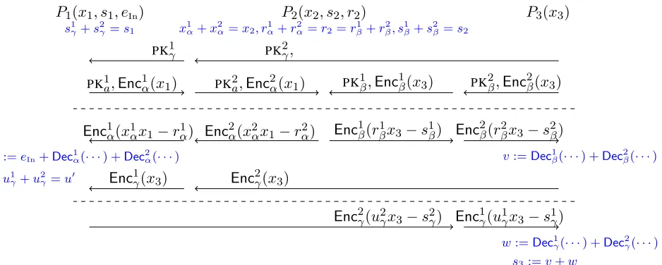
Definition2.3. The details of our protocol are as follows. We usually assume that randomness is implicit in the encryption scheme, unless specified explicitly. See Figure3for a high level description of protocol ΠDMULT.

Protocol 1 (3-bit Multiplication protocolΠDMULT)

Input & Randomness: Parties P1, P2, P3 are given inputs(x1, eIn), x2, x3, respectively. P1 chooses a random bits1 andP2 chooses two random bitss2, r2 (in addition to the randomness needed for the sub-protocols below).

ROUND 1:

– PartyP1runs key generation twice,(PK1a,SK1a),(PK2a,SK2a)←Gen, encryptsCα1[1] :=EncPK1a(x1) andC2_α[1] :=EncPK2a(x1), and broadcasts((PK

1

a,C1α[1]),(PKa2,C2α[1]))(to be used byP2).

– P3runs key generation four times,(PK1_β,SK1_β),(PK2_β,SK2_β),(PK1γ,SK1γ),(PKγ2,SK2γ)←Gen(1κ).

Next it encrypts using the first two keys, C1_β[1] := Enc_PK1

β(x3) and C

2

β[1] := EncPK2_β(x3),

and broadcasts (PK1_β,C_β1[1]), (PK2_β,C2_β[1]) (to be used byP2), and (PK1γ,PK2γ) (to be used in round 3 byP1).

– Each partyPj samples random secret shares of 0, (z_j1, z2_j, z_j3) ← Share(0,3)and sendszi_j to partyPiover a private channel.

ROUND 2:

– PartyP2 samplesx1α, xα2 such thatx1α+x2α = x2 andr1α, r2α such thatr1α+rα2 = r2. It use affine homomorphism to computeC1_α[2] := (x1_α C1_α[1])r_α1 andC2_α[2] := (x2_α C2_α[1])r2_α.

PartyP2also samplesr1β, r2βsuch thatr1β+r2β =r2ands1β, s2βsuch thats1β+s2β =s2, and uses affine homomorphism to computeC1_β[2] := (r1_β C1_β[1])s1_βandC2_β[2] := (r_β2 C2_β[1])s2_β.

(19)

– PartyP3 encryptC1γ[1] := EncPK1γ(x3)andC

2

γ[1] := EncPK2γ(x3)and broadcast(C

1

γ[1],C2γ[1]) (to be used byP1).

ROUND 3:

– PartyP1computesu:=DecSK1a(C

1

α[2]) +DecSK2a(C

2

α[2])andu0 =u+eIn.

ThenP1samplesu1γ, u2γsuch thatu1γ+u2γ=u0ands1γ, s2γsuch thats1γ+s2γ=s1. It uses affine homomorphism to computeC1_γ[2] := (u1_γ C1_γ[1])s1_γandC2_γ[2] := (u2_γ C2_γ[1])s2_γ.

P1 broadcasts(C1γ[2],C2γ[2])(to be used byP3).

DEFENSE: At this point, the adversary broadcasts its “defense:” It gives an input for the protocol, namelyx?. For every “OT protocol instance” where the adversary was the sender (the one sending

C?_?[2]), it gives all the inputs and randomness that it used to generate these messages (i.e., the val-ues and randomness used in the affine-homomorphic computation). For instances where it was the receiver, the adversary choosesone message of each pair(eitherC1_?[1]orC2_?[1]) and gives the inputs and randomness for it (i.e., the plaintext, keys, and encryption randomness). Formally, lettransbe a transcript of the protocol up to and including the3rdround

transdef=

PK1_a,C1_α[1],C1_α[2],PK2_a,C2_α[1],C2_α[2], PK1_β,C1_β[1],C1_β[2],PK2_β,C2_β[1],C2_β[2],

PK1_γ,C1_γ[1],C1_γ[2],PK2_γ,C2_γ[1],C2_γ[2]

transb P1

def

= PKb_a,Cb_α[1], C1_γ[2],C2_γ[2]

trans0_P

2 =trans 1 P2

def

= C1_α[2],C2_α[2], C1_β[2],C2_β[2]

transb_P

3 def

= PKb_β,Cb_β[1], PKb_γ,Cb_γ[1]

we have three NP languages, one per party, with the defense for that party being the witness:

L_P₁ =        trans

∃(x1, eIn, ρα,SKa, σα, u1γ, u2γ, s1γ, s2γ)

s.t.

(PK1a,SKa=Gen(ρα)∧C1α[1] =EncPK1_a(x1;σα))

∨(PK2a,SKa=Gen(ρα)∧C2α[1] =EncPK2_a(x1;σα))

∧ C1γ[2] =u1γ C1γ[1]s1γ ∧ C2γ[2] =u2γ C2γ[1]s2γ        (2)

L_P₂ =    trans

∃(x1_α, x2_α, s1_β, s_β2, r_α1, r2_α, r_γ1, r2_γ) s.t. r1_α+r2_α=r1_γ+r_γ2

∧ C1α[2] =x1α C1α[1]r1α ∧ C2α[2] =x2α C2α[1]r2α

∧ C1β[2] =r 1 β C

1

β[1]s 1 β ∧ C

2

β[2] =r 2 β C

2

β[1]r 2 β    (3)

LP3 =              trans

∃(x3, ρβ,SKβ, σβ, ργ,SKγ, σγ)

s.t. (PK

1

β,SKβ =Gen(ρβ)∧C1β[1] =EncPK1

β(x3;σβ))

∨(PK2β,SKβ=Gen(ρβ)∧C2β[1] =EncPK2

β(x3;σβ)) !

∧

(PK1γ,SKγ=Gen(ργ)∧C1γ[1] =EncPK1_γ(x3;σγ)) ∨(PK2γ,SKγ=Gen(ργ)∧C2γ[1] =EncPK2_γ(x3;σγ))

             (4)

ROUND 4:

– P3computesv:=DecSK1_β(C 1

β[2]) +DecSK2_β(C 2

β[2]),w:=DecSK1_γ(Cγ1[2]) +DecSK2_γ(C2γ[2]), and

s3:=v+w.

(20)

P2(x2, s2, r2) x1α+x2α=x2, r1α+r2α=r2=rβ1+r

2 β, s

1 β+s

2 β=s2 s1γ+s2γ=s1

P3(x3)

P1(x1, s1, eIn)

PK1_a,Enc1_α(x1) PKa2,Enc2α(x1) PK2β,Enc 2 β(x3)

PK1_β,Enc1_β(x3)

PK1_γ PK2_γ,

Enc1_α(x1_αx1−r1α) Enc2α(x2αx1−rα2) Enc 2

β(r2βx3−s2β)

Enc1_β(r_β1x3−s1_β)

u0:=eIn+Dec1α(· · ·) +Dec2α(· · ·)

u1γ+u2γ=u0 Enc_γ1(x3) Enc2γ(x3)

Enc1_γ(u1_γx3−s1γ)

Enc2_γ(u2_γx3−s2γ)

v:=Dec1β(· · ·) +Dec 2 β(· · ·)

w:=Dec1γ(· · ·) +Dec2γ(· · ·) s3:=v+w

Figure 3:Round 1, 2 and 3 ofΠDMULTprotocol. In the fourth round each partyPiadds the zero shares tosjand broadcasts the

result.

• OUTPUT:All parties set the final output toZ =S1+S2+S3.

Lemma 3.1 ProtocolΠDMULTsecurely realizes the functionalityFA

MULT(cf. Figure2) in the presence of a

“defensible adversary” that always broadcasts valid defense at the end of the third round.

Proof: We first show that the protocol is correct with a benign adversary. Observe thatu0 =eIn+x1(x1α+

x2_α)−(r_α1 +r2_α) =eIn+x1x2−r2,and similarlyv=x3r2−s2andw=x3u0−s1. Therefore,

S1+S2+S3 =s1+s2+s3 =s1+s2+ (v+w)

=s1+s2+ (x3r2−s2) + (x3u0−s1) =x3r2+x3(x1x2−r2+eIn)

= (x1x2+eIn)x3

as required. We continue with the security proof.

To argue security we need to describe a simulator and prove that the simulated view is indistinguishable from the real one. Below fix inputsx1, eIn, x2, x3, and a defensible PPT adversary Acontrolling a fixed subset of partiesI ⊆[3](and also an auxiliary inputz).

The simulator S chooses random inputs for each honest party (denote these values by xbi), and then follows the honest protocol execution using these random inputs until the end of the 3rd round. Upon receiving a valid “defense” that includes the inputs and randomness that the adversary used to generate (some of) the messagesCi_?[j], the simulator extracts from that defense the effective inputs of the adversary to send to the functionality, and other values to help with the rest of the simulation. Specifically:

• IfP3 is corrupted then its defense (for one of theCi_β[1]’s and one of the Ciγ[1]’s) includes a value forx3, that we denotex∗3. (A defensible adversary is guaranteed to use the same value in the defense forC?

β[1]and in the defense forC ? γ[1]’s.)

(21)

some valuesr2, s2. (IfP2is honest then byr2, s2we denote below the values that the simulator chose for it.)

• IfP1is corrupted then its defense (for either of theCiα[1]’s) includes a value forx1that we denotex∗1. From the defense for bothC1_γ[2],C2_γ[2]the simulator learns theuγ_i’s andsγ_i’s, and it setsu0:=u1_γ+u2_γ

ands1 :=s1γ+s2γ.

The simulator setsu := x∗₁x∗₂−r2 ifP2 is corrupted andu := x∗1xb2−r2 ifP2 is honest, and then computes the effective valuee∗In := u

0 ₋_u_{. (If}_P

1 is honest then bys1, u, u0 we denote below the values that the simulator used for it.)

Letx∗_i ande∗Inbe the values received by the functionality. (These are computed as above if the corresponding party is corrupted, and are equal toxi, eInif it is honest.) The simulator gets back from the functionality the answery = (x∗₁x∗₂+e∗In)x

∗ 3.

Having values fors1, s2as described above, the simulator computess3 :=y−s1−s2 ifP3 is honest, and ifP3 is corrupted then the simulator setsv := r2x∗3 −s2, w := ux∗3−s1 ands3 := v+w. It then proceeds to compute the valuesSj that the honest parties broadcast in the last round.

Letsbe the sum of thesivalues for all the corrupted parties, and letzbe the sum of the zero-shares that the simulator sent to the adversary (on behalf of all the honest parties), andz0be the sum of zero-shared that the simulator received from the adversary. The values that the simulator broadcasts for the honest parties in the fourth round are chosen at random, subject to them summing up toy−(s+z−z0).

If the adversary sends its fourth round messages, an additive output error is computed as eOut :=

y−P

jS˜j where S˜j are the values that were broadcast in the fourth round. The simulator finally sends (deliver, eOut)to the ideal functionality.

This concludes the description of the simulator, it remains to prove indistinguishability. Namely, we need to show that for the simulatorSabove, the two distributionsREALΠDMULT,A(z),I(κ,(x1, eIn), x2, x3) and IDEAL_FA

MULT,S(z),I(κ,(x1, eIn), x2, x3) are indistinguishable. We proceed in several hybrid games, beginning fromH0 that has view identical to the real game, and ending at H8 whose view is distributed

identically to the simulation.

High-level sketch of the proof.On a high-level, in the first two intermediate hybrids, we modify the fourth message of the honest parties to be generated using the defense and the inputs chosen for the honest parties, rather than the internal randomness and values obtained in the first three rounds of the protocol. Then in hybridH3 below we modify the messages Si that are broadcast in the last round. Next, in hybridH4, we

modify P3 to use fake inputs instead of its real inputs where indistinguishability relies on the semantic security of the underlying encryption scheme. In hybrid H5, the value u is set to random u0 rather than

the result of the computation usingC2_α[1]andC2_α[2]. This is important because only then we carry out the reduction for modifyingP1’s input inH6. Indistinguishability fromH4toH5 follows from the equivocation

property of the encryption scheme, whereas, fromH5toH6 security relies on the semantic security. Then,

in hybridH7, we modify the input ofP2from real to fake which again relies on the equivocation property. Finally inH8 we modify theSi’s again to use the output from the functionalityFMULTA which is a statistical argument.

We proceed in several hybrid games, beginning fromH0 that has view identical to the real game, and

ending atH8whose view is distributed identically to the simulation.

(22)

HybridH0. This experiment is the execution in the real world. As usual, we postulate a centralized “chal-lenger” that plays the role of the honest parties inH0, namely it gets all their inputs and just follows the

protocol on their behalf (and ignores the “defense” provided by the adversary).

HybridH1. In the next few hybrids we make some changes to the internal computations of the challenger without affecting what the adversary sees. In this hybrid, if P1 is honest then instead of choosing s1 at random and then choosing random s1,2γ that add up to s1, the challenger chooses boths1,2γ uniformly at random and setss1 := s1γ+s2γ. Similarly, ifP2 is honest then the challenger chooses at randoms1,2_β ,rα1,2, andr_β1, and setss2:=s1_β+s2_β,r2 :=r1α+rα2, andrβ2 :=r2−rβ1.

Also, the challenger in this hybrid no longer ignores the adversary’s defense, instead it uses it to compute some local variables (which are then ignored). Specifically, regardless of which party is corrupted, the challenger knows:

• A value forx1 (either sinceP1is honest, or from the defense of one of theC1α,2[1]’s).

• Theu1,2γ ands1,2γ ’s (either sinceP1is honest, or from the defense of both theC1γ,2[2]’s).

• Thex1,2_β ,r_β1,2,rγ1,2, and,s1,2_β ’s (either sinceP2 is honest, or from the defense of all theC1_α,β,2[2]’s).

• A value forx3 (eitherP3is honest, or from the defense of one of each of theC_β1,2[1]’s andC1γ,2[1]’s).

Below we denote s1 := s1γ +s2γ andu0 = u1γ+u2γ, whether or not P1 is honest. Similarly, we denote

r2 :=r_β1+r_β2 =r1γ+rγ2ands2:=s1_β+s2_β, whether or notP2is honest.

The challenger in H1 also chooses random “fake input bits”xbi for the parties (in addition to the real inputsxi). These inputs are never used inH1, but will be used in some of the hybrids below.

HybridH2. In this hybrid, the challenger forgoes decrypting the ciphertextsC1_β,γ,2[2]even if P3 is honest. Whether or notP3 is honest, at the end of the3rdround the challenger uses the values above that it knows to setv:=r2x3−s2,wi:=uiγx3−siγ (i= 1,2), andw:=w1+w2.

WhenP3is honest,C1_β,γ,2[1]are all valid ciphertexts. Therefore so areC1_β,γ,2[2], since they all have a valid

defense. Moreover the valid defense implies thatr1,2_β , u1,2γ ands1,2_β,γare consistent with the plaintext values inside these ciphertexts. Hence the computed valuesv, ware identical to what was computed inH1(in the case thatP3 is honest).

HybridH3.This hybrid changes the computation of thesi’s:

• IfP1 is honest then the challenger changes the way it computess1: Rather thans1 := s1γ+s2γ, the challenger waits until after the3rdround, then setss1:= (x1x2+eIn)x3−s2−v−w(and broadcasts

S1 =s1+Pjzj1on behalf ofP1). It is easy to check thats1in this hybrid is the same as inH2: As

u0 =u1_γ+u2_γ =x1x2+eIn−r2, then

(x1x2+eIn)x3−s2−v−w = (x1x2+eIn)x3−s2−(r2x3−s2)− u0x3−(s1γ+s2γ)

= (x1x2+eIn)x3−r2x3−(x1x2+eIn−r2)x3+s1γ+s2γ = s1γ+s2γ.

• IfP1is corrupted andP2 is honest, then the challenger changes the way it computess2: Rather than

(23)

• IfP1 andP2 are corrupted andP3is honest, the challenger changes the way it computess3: Rather thans3 :=v+w, the challenger sets after the3rdrounds3 := (x1x2+eIn)x3−s1−s2and broadcasts

S3 =s3+P_jzj3on behalf ofP3. As in the other two cases, here toos3is the same as inH2.

HybridH4.In this hybrid, ifP3is honest then the challenger encrypts the fakexb3rather than the realx3in all the ciphertextsC1_β,γ,2[1]. The rest of the execution remains unchanged (including using the realx3 in the computation ofv, w, s3as above).

Recall that the challenger no longer decrypts any of the ciphertextsC1_β,γ,2[2]and hence no longer uses the

secret keysSK1,2_β ,SK1,2γ . We can therefore reduce indistinguishability betweenH3 andH4 to the semantic security of the encryption. The reduction algorithm plays the challenger, but instead of generating the keys itself and doing the encryption, it receives the public keys and ciphertexts from the CPA-security game, where theC1_β,γ,2[1]’s encrypt eitherx3orxb3. Hence we have:

Claim 3.2 Assuming semantic security ofEnc, the adversary’s view inH4is indistinguishable fromH3.

HybridH5.IfP1is honest, the challenger changes the way it chooses theu1,2γ ’s: Instead of choosing them at random subject tou1_γ+u2_γ =u0, they are chosen uniformly and independently.

We note that in this hybrid the challenger no longer needs to computeuandu0, and therefore it no longer needs to decrypt the ciphertextsC1_α[2],C2_α[2].

Claim 3.3 IfEncsatisfies the equivocation property from Definition2.5, then the adversary’s view in hybrid

H5is statistically close to the hybridH4.

Proof: Below we prove Claim3.3for the case whereC1

γ[1] is a valid ciphertext, encrypting thex3 that the challenger knows. The proof for the case whereC2_γ[1]is a valid encryption ofx3 is symmetric, and we know that at least one of these cases hold since the adversary is defensible.

Below we fix all the inputs and randomness of all the parties except the choices of u1

γ and s1γ and whatever randomness is involved in computingC1_γ[2] := (u1_γ C1_γ[1])s1_γ. We show that whenC1_γ[1]is a valid encryption ofx3, the adversary’s views in the two hybrids are statistically close, even conditioned on all these fixed values.

We note that the fixed values include in particularu2_γ, ands2_γ, and conditioned on all those values the adversary’s view is uniquely determined byC1_γ[2]ands1. It is therefore sufficient to show that the residual distributions on(C1_γ[2], s1)are close between these hybrids. We next show that boths1 andC1γ[2]depend only on the single valuew1:=u1γ·x3−s1γ.

Fors1, since everything exceptu1_γands1_γis fixed, then in particular∆ := (x1x2+eIn)x3−s2−v−w2is fixed, sos1 := ∆−w1is uniquely determined byw1. ForC1γ[2], the equivocation property of the encryption scheme implies in particular that for any validC1_γ[1] =Enc(x3), the distribution ofCγ1[2] :=u1γ C1γ[1]s1γ depends (up to negligible difference) on just the value encrypted in it, namely byw1:=u1γ·x3−s1γ.8

We conclude that it is sufficient to show thatw1 has the same distribution in both hybrids. But this is obvious, as in both hybrids it is set asw1 :=u1γ·x3−s1γfor a uniformly randoms1γ, and only the choice of

u1_γdiffers between them.

HybridH6. IfP1 is honest, the challenger encrypts the fakexb1 rather than the realx1 in the ciphertexts

C1α,2[1]. The rest of the execution remains unchanged (including using the realx1in the computation ofs1).

8

This is where we use the assumption about the validity ofC1

Round-Optimal Secure Multi-Party Computation

Round-Optimal Secure Multi-Party Computation

Contents

1

Introduction

2

Additional Preliminaries

3

Warmup MPC: The Case of Defensible Adversaries