Overview of major processes and mechanisms affecting the mercury cycle on different spatial and temporal scales

c

Owned by the authors, published by EDP Sciences, 2010

Overview of major processes and mechanisms affecting the

mercury cycle on different spatial and temporal scales

N. Pirrone1,2,a_{, I.M. Hedgecock}2_{, S. Cinnirella}2_{, and F. Sprovieri}2

1 _{CNR-Institute of Atmospheric Pollution Research, Rome, Italy}

2 _{CNR-Institute of Atmospheric Pollution Research, Division of Rende, 87036 Rende, Italy}

Abstract. Mercury emissions to the atmosphere and its transport, transformation and deposition to and re-emission from terrestrial and aquatic ecosystems on hemispherical and global scales has received increasing attention from both the scientific and the regu-latory communities during the last twenty years. It is well known that the atmosphere is the major transport media through which mercury is redistributed on global scale once it is released from point and diffuse emission sources. A substantial amount of research has been carried out worldwide aiming to assess the relationships between emissions from natural vs. anthropogenic sources, inter-hemispherical atmospheric transport patterns, and atmospheric deposition to and re-emission from oceans, its bioaccumulation in fish, and evaluation of policy strategies to reduce the impact of mercury emissions on human health and ecosystems. This chapter provides a highlight of key aspects related to mercury contamination, including: a) major processes affecting the mercury cycle between the atmosphere and aquatic and terrestrial ecosystems, b) mercury emissions from natural and anthropogenic sources, c) spatial and temporal distributions and trends of mercury species over the northern and southern hemispheres, d) the chemical and physical processes affecting the transport and fate of atmospheric mercury, and e)major policy frameworks aiming to control the impact of mercury on human health and ecosystems.

1 Introduction

Mercury is ubiquitous in the atmosphere, it has ground level background concentrations which are almost constant over hemispheric scales; the southern hemisphere having a slightly lower concen-tration than the northern. Mercury is emitted into the atmosphere from a variety of anthropogenic and natural sources. Of the anthropogenic sources, among the most important are fossil fuel com-bustion, smelting, cement production and waste incineration, while the oceans are the largest natural source of Hg to the atmosphere, volcanism also makes an important contribution [1–6]. Most mer-cury emissions are of elemental Hg but anthropogenic emissions also include Hg in different chemical and physical forms. Mercury cycling between different environmental compartments depends on the dynamic of chemical and physical processes (i.e. oxidation and reduction, dry deposition, wet scav-enging/depostion, re-emission and methylation,) which influence its transport and residence time in the global environment. Due to intensified anthropogenic emission of mercury into the atmosphere since the beginning of industrialization this global Hg pool has increased in the past 150 years, evidence suggests that the global atmospheric burden has increased by a factor of 3 to 5 for example. Recent measurements of free tropospheric air, from high altitude sites and from measurements made on board

a_{e-mail:[email protected]}

This is an Open Access article distributed under the terms of the Creative Commons Attribution-Noncommercial License 3.0, which permits unrestricted use, distribution, and reproduction in any noncommercial medium, provided the original work is properly cited.

aircrafts indicate that the elemental Hg concentration changes little up to the tropopause, although events in which higher than usual concentrations of oxidised Hg species are observed do occur [7–9]. In the stratosphere mercury has been identified associated with stratospheric aerosols [10], and almost total depletion of elemental Hg recorded [11]. Therefore, mercury is found in the boundary layer, in the free troposphere and stratosphere; and the transport and fate of mercury is determined by the differ-ent chemical, physical and meteorological environmdiffer-ents presnt in these regions of the atmosphere and also by the exchange between them [9]. Evidence of long-term changes in the atmospheric mercury burden have been derived from chemical analysis of lake sediments, ice cores, peat deposits and firm air records [7, 9, 12–14]. These studies identify a peak in the atmospheric mercury concentration dur-ing the 70s in the Northern Hemisphere. A growdur-ing number of these records from both hemispheres demonstrate approximately a threefold increase of mercury deposition since pre-industrial times [9]. In principle, an increase in the global atmospheric pool should also be reflected in the background concentration. However, since the first reliable measurement data were published just 30 years ago, it is extremely difficult to determine a global trend from the existing spatially and temporally inchoate air concentration data sets. For example, Asian mercury emissions are believed to have rapidly increased over the last decade [2, 15], however, this is not reflected either in the long-term measurement of Total Gaseous Mercury (TGM) at Mace Head, Ireland covering the period between 1996 to 2006 [16, 17], nor in the precipitation data of the North American Mercury Deposition Network (MDN). Recognizing that TGM and the Hg flux to the earth’s surface in dry and wet deposition are spatially heterogeneous, several initiatives have aimed to set up monitoring networks in order to compare trends between sites in the same region, between regions, and to determine the influence of local and regional emission sources. There is also interest in understanding the processes that contribute to Hg species concentration variability on a diurnal, weekly, seasonal, and annual basis. In 1995, Fitzgerald [18] argued for and defined the basic requirements of an Atmospheric Mercury Network (AMNet). This has partly been accomplished on a regional scale within the Canadian Atmospheric Mercury Network (CAMNet), which may be considered as seminal in this respect. Part of the CAMNet contributes also to the Arctic Monitoring and Assessment Program (AMAP) under the Ministry Council of Circum Polar Countries and where there are also contributions from the Scandinavian countries. Neverthe-less, although the number of atmospheric Hg monitoring stations has increased [19], the database is sparse, especially in remote locations suitable for the assessment of the trend in background Hg con-centrations. In Europe atmospheric mercury measurements have been performed since the early 80s at selected northern European sites as part of the European Monitoring Evaluation Program (EMEP) of the UNECE-LRTAP convention. This network detected the decrease in atmospheric Hg concentrations and Hg in precipitation which occurred when Eastern European countries went into economic decline in the late 1980’s leading to the closure of a significant number of industrial installations. Later, as part of three European Commission funded projects, (MAMCS, MOE and MERCYMS) a first attempt was made to establish an European wide measurement network. One of the major outcomes of these EU projects was that for the first time, simultaneous measurements of speciated mercury were performed at 10 measurement sites located across Europe during several two-week intensive campaigns at both ground-based and off-shore sites [20–24]. The results of these projects allowed, among other things, the preparation of the European Position Paper on Mercury [25] which provided the scientific back-ground of the 4th _{Daughter Air Quality Directive. One of the major findings of these projects was a}

affecting the transport and fate of atmospheric mercury, and e)major policy frameworks aiming to control the impact of mercury on human health and ecosystems.

2 The mercury cycle

The global mercury cycle is a natural phenomenon which has been enhanced by anthropogenic activ-ity. Mercury enters the atmosphere, oceans, rivers and soils, and eventually also biota from a number of natural processes. The most important of these is volcanic activity, but the weathering of Hg bearing rocks also adds to the global environmental Hg burden over time. The natural Hg cycle should not be considered to be constant in time, as major volcanic eruptions can, over a short period, add quite signifi-cant quantities of Hg to the atmosphere which is then deposited over time to both aquatic and terrestrial surfaces. Clearly the spatial distribution of Hg is not homogeneous over the earth either, depending as it does on the location of volcanic sources and Hg rich soils. Mercury released to the atmosphere and oceans is transported, relatively quickly in the atmosphere and significantly less so in the oceans, and it is the atmosphere therefore that is the major pathway by which Hg is distributed around the globe. The apparent residence time of Hg in the atmosphere (with its present day composition) is around 8 months [30], although it does vary, depending on source location and atmospheric condi-tions. Mercury has enough time to redistributed on a global scale, and Hg is currently found to have a very uniform background concentration on a hemispheric scale [29], although as discussed below this may be due to rapid cycling at interfaces rather than uninterrupted transport from source to receptor [31]. The global scale redistribution of emitted Hg is aided by its exchange between environmental compartments. Mercury in the atmosphere can be deposited to the oceans or to land, but this deposited Hg can be re-emitted to the atmosphere, hours, weeks or decades later. Mercury taken up by fish or trees for example, may be released again years or centuries later as the dead organism decays. Thus the presence of Hg in the environment is prolonged by its continual passing from one environmental compartment to another until eventually, Hg associated with marine particulate matter, settles and is buried in deep ocean sediments [32, 33].

The major exposure pathway to Hg contamination for humans is through the consumption of preda-tory fish. As stated above however, the major transport/redistribution pathway for environmental Hg is the atmosphere. The relationship between atmospheric deposition and the concentrations of Hg in aquatic environments, as well as that between Hg concentrations in water and those in fish need to be understood. One important factor in this exchange between the atmosphere, water and biota is the time that it takes for one environmental compartment to respond to a change in the state of another. For example, if a lake is considered, there is a balance between atmospheric input, Hg concentration (and speciation) in the water, Hg concentration (and speciation) in sediments at the bottom of the lake and the Hg concentration in the lake biota both in the water and in the sediments. Reducing the Hg deposition to the lake from the atmosphere will set offa process of re-equilibration of the Hg present in the system between the various environmental reservoirs and it is possible to envisage over time that the average quantities of Hg in each of them will diminish. The extent of the reduction of Hg concentrations in fish is of interest as this is directly related to possible health risks from exposure, as is the time required for this new steady state to be attained. This is an oversimplification of the actual problem, larger (older) fish would generally have higher Hg concentrations in their tissues, and other physico-chemical factors may change the rate at which Hg is exchanged between environmen-tal compartments and the form in which it is present. However it illustrates the point that because of the significant, order or orders of magnitude differences in the time scales of the processes (transport, exchange, re-exchange and removal), within the environmental global Hg cycle; it is not a simple matter to conclusively link sources to receptors, or changes in the Hg burden of one environmental compartment to changes in another. This point is discussed further later in Sect. 2.6).

global environmental burden was the result of Hg extraction and use, and was mostly on a limited scale. The emissions from these activities were generally relatively limited in quantity and rather like natural emissions were mostly from quite distinct geographical locations. During the industrial revolution the previous direct association of Hg emission with mostly metallurgical processes began to change. Mercury use, and therefore emission became more widespread across industry and manufacture, and, as we now know, the coal combustion that provided the energy required by industry, was itself a source of Hg emission, due to the trace amounts of Hg found in coal.

2.1 The present day atmospheric Hg cycle

The perturbation caused by industrial activity is estimated to have increased the global atmospheric Hg burden by 3 to 5 times its pre-industrial level [32, 34]. The increased deposition of Hg from the atmosphere has resulted in an estimated doubling of the emissions from land and oceans. The current contribution of oceanic Hg emissions to the atmosphere is roughly the same as that from anthropogenic sources [2, 4], and possibly nearly 90% of oceanic emissions are re-emissions [35]. The global background concentration of atmospheric Hg differs between the northern and southern hemi-spheres. This fact is indicative of both the greater industrial activity in the northern hemisphere and also the atmospheric lifetime of mercury which, while it is long enough for Hg to be evenly distributed hemispherically, it is not long enough to survive the longer times required for cross equator transport. The blocking of atmospheric tracer transport across the equator does not precisely coincide with either the geographical equator or the position of the ITCZ, however it is very distinct and has been coined “the chemical equator” [36]. In terms of the interaction of the atmospheric Hg cycle and the oceanic Hg cycle this hemispheric background concentration difference is a very important clue to the exchange of Hg between the atmosphere and the oceans. The continued higher atmospheric concentration of Hg in the northern hemisphere suggests that the Hg deposited to the oceans does not remain in the ocean long enough for the global ocean circulation to redistribute Hg evenly across the globe. This points to a multi-hop transportation mechanism for Hg, where deposition and re-emission occur on a reasonably short time-scale [26], which tallies with the estimate of [35] that 90% of Hg deposited to the oceans is re-emitted. The impact of reductions in emissions to the atmospheric Hg burden was demonstrated in post-Soviet Europe when a large number of coal fired power stations in the former Eastern-bloc were shut down. This led to a relatively rapid sudden and quantitatively significant regional decrease in Hg emissions to the atmosphere. Observations of atmospheric Hg concentrations and Hg deposi-tion in precipitadeposi-tion form monitoring sites in the Netherlands, Germany, Norway and Sweden, showed that in spite of no change in the measured Total Gaseous Mercury (TGM) concentration, there was a clear decrease in Hg deposition in rainfall, over the period 1995-2002 [37]. Earlier measurements [38] showed that TGM values at these sites had decreased until the early 90s, when they levelled off, suggesting that TGM became more influenced by the Hg(0) global background, while deposition continued to be influenced by by regional emissions of Hg(II) and Hg(P). The opposite scenario, of above background concentrations of Hg(0), influenced by regional emissions is seen at Hedo Station, Okinawa, where outflow from Asia can be detected [39]. The same outflow also influences concen-trations of Hg at the Mount Bachelor Observatory in Oregon [8]. Thus the atmosphere, on a regional scale, actually appears to respond quite rapidly to changes in emissions. However, the lack of long-term Hg concentration and deposition data mean that up until now there are limited instances where this supposition can be tested.

2.2 The present day Oceanic Hg Cycle

as Hg(0), Hg(II), methylmercury and dimethylmercury as well as associated with particulate matter, sometimes referred to as colloidal mercury. The methylation processes at work in the oceans are not fully understood but is known to occur in the sediments of coastal shelf and esturine regions. It also occurs within the water column and at deep ocean hydrothermal vents, the amount of MeHg in water varies from 5-35% of the total. The reduction of deposited Hg(II) to Hg(0) by biological and photolytic processes in the surface waters of the oceans plays an extremely important role in the atmospheric redistribution of Hg around the globe. A recent modelling study of the oceanic Hg cycle which took into account the surface, intermediate and deep waters of the major ocean basins, and the vertical and lateral movement of water between them, including major zones of upwelling and areas of overturning, indicated that the ocean Hg burden is as yet far less perturbed than that of the atmosphere [32]. The same study also highlighted the importance of direct from rivers which directly impact estuaries and shallow continental shelf regions. The ocean compartment most perturbed from pre-industrial times in the model was the surface North Atlantic (and Mediterranean) whilst the deep Pacific was the least influenced.

2.3 Fresh water Hg cycling

Lake sediments and wetland areas are important areas of Hg methylation. These areas are influenced by both atmospheric deposition and run-offfrom their surrounding watersheds. Numerous lakes in N. America have advisories regarding the consumption of fish caught in lakes, and these lakes are by no means all influenced by major local sources. The Hg cycle in lake environments is more complex than the ocean and methylation can be influenced by sediment type, dissolved organic carbon content, pH, iron, and sediment type and structure. Of all factors though the most important is often sulphate as many of the bacteria that methylate Hg are sulphate reducing bacteria [41]. A coupled ecosystem modelling study of the effect of decreased Hg deposition on different freshwater ecosystem types, sug-gests that where the major mercury input is direct atmospheric deposition, the response of the system to the changes is most rapid, whereas those ecosystems receiving Hg from the watershed respond more slowly [42]. All the ecosystem types studied however, showed an initial rapid decline of 20 to 60% in Hg concentrations over one to three decades. A recent study suggests that the relationship between atmospheric inorganic Hg and methylmercury in fish is linear and theat the response to changes in deposition occurs rapidly (within weeks) [43].

2.4 Terrestrial Hg cycling

With the exception of areas which are rich in Hg bearing minerals, most Hg in soils and vegetation comes originally from atmospheric deposition, both wet and dry. Hg(II) deposits on leaves and from the atmosphere, whereas uptake by plants of Hg(0) is thought to occur through the stomata. Most Hg in the terrestrial system however is in soils rather than biomass, and it is generally bound to organic substances such as compounds with reduced sulphur groups. Mercury reaches the soil in vegetated areas via direct precipitation and throughfall. Litterfall also adds to the Hg contained in soils. Mercury contained in soils can be reduced, this is generally thought to be an abiotic process and appears to be influenced by temperature and solar radiation. Some evidence that Hg emission is enhanced from dry soil has been found. It has recently been proposed that a significant part of the Hg(II) deposited to terrestrial surfaces is reduced and rapidly returns to the atmosphere, mirroring then the multi-hop mechanism of distribution of Hg suggested for the oceanic Hg cycle. The evidence for this ’prompt-recycling’ as it has been termed [33] comes from measurements made during the METALLICUS experiment [44], from observations of Hg fluxes (and Hg concentrations in snow) after AMDEs as well as indirectly from modelling studies. Natural emissions and terrestial cycling are further discussed in Sect. 3.1.3.

2.5 Putting numbers on burdens and fluxes

Fig. 1. The most recent esimate of the environmental pre-industrial and present day Hg burden and the natural

and anthropogenic annual fluxes (Mg year−1_{). Pre-industrial burdens and fluxes are in black, the anthropogenic}

burdens and fluxes in red, reproduced from Selin [31].

burdens in these estimates do not vary wildly, however the fluxes between them appear to be less well constrained. The estimates of the pre-industrial atmospheric Hg burden range between 1,600 and 2,050 Mg, while the anthropogenic atmospheric contribution ranges between 3,400 and 4,000 Mg, to give totals between 5,000 and 5,600 Mg. Estimated pre-industrial fluxes of Hg to the atmosphere from the ocean vary between 400 and 2,040 Mg year−1, while the estimates of the anthropogenic component of the ocean to atmosphere Hg flux span 400 to 2,960 Mg year−1_{. The major differences in the Hg flux} estimates to date do not depend on assessments of total burdens but the ease and rapidity with which Hg is cycled between environmental compartments. Generally speaking it seems that the more recent the Hg global cycle estimate the higher the exchange fluxes, reflecting the growing understanding of the the dynamic way in which Hg is cycled in the environment, and also an ever increasing technical capacity to determine Hg concentrations and fluxes in the environment. The most recent assessment of the global Hg cycle by Selin [33] is reproduced graphically in Fig. 1. It should be noted that of all the assessments to date this one has the highest burdens and the most active cycling between environ-mental compartments.

2.6 The response time of environmental compartments to flux changes

in part attributable to anthropogenic emissions in North America and Europe. It is important to know what to expect in terms of ecosystem response from any proposed emission reduction strategy. In their modelling study of the ocean cycle of Hg Sunderland et al. [32] estimated how close the current Hg concentrations are to their steady state values and also how long it would take, if emissions continue at their present rate, for each ocean compartment that they considered. The estimated times varied from 10 to 1000, years. This information is useful, because although monitoring atmospheric Hg con-centrations would in the first instance permit the evaluation of emission reduction, it is in marine and fresh water ecosystems that the concentration of Hg matters most. Understanding the time lag between emission change, atmospheric response and aquatic ecosystem response would therefore be essential in judging the efficacy of any future emissions reduction policy.

3 Emissions from natural and anthropogenic sources

Assessments of mercury emission from natural and anthropogenic sources increase their attraction to researchers as of the uncertainty in the estimate of origin and distribution in time and space of mercury release to the atmosphere. Twenty years of research have experienced significant advances in assess-ment of mercury emission from anthropogenic sources, whereas a small attention was kept on mercury emission from natural sources. In details, earlier studies of global mercury emissions were aimed pri-marily to assess the contribution from anthropogenic sources, namely coal, oil and wood combustion, solid waste incineration, pyrometallurgical processes [1, 5, 45, 46] as well as artisanal small scale gold mining [47, 48]. On the other hand, several studies have estimated emissions from volcanoes [3, 49, 50], re-emission from oceans and surface waters [34], top soil and vegetation [51] and forest fires [52–55]. More recently, assessments of mercury emissions to the global atmosphere have included the con-tribution of the most important anthropogenic and natural sources [2, 6, 56, 57]. This section of the chapter reports most recent advances on global assessments on mercury emissions from natural and anthropogenic sources.

3.1 Natural sources

The estimate of mercury emissions from natural sources include the contribution from primary nat-ural sources and reemission processes of historically deposited mercury over land and sea surfaces. The mercury emitted from volcanoes, geothermal sources and topsoil enriched in mercury pertains to primary natural sources, whereas the re–emission of previously deposited mercury on vegetation, land or water surfaces is primarily related to land use changes, biomass burning, meteorological conditions and exchange mechanisms of gaseous mercury at air-water/top-soil/snow-ice pack interfaces [4, 20].

3.1.1 Volcanoes and geothermal activities

The contribution of volcanoes varies over time depending whether they are in a degassing or erup-tion phase. The Hg/SO2 mass ratio is generally adopted to estimate mercury emissions, though this approach is very controversial because of the paucity of relevant data and their variability [49, 50]. On average, volcanoes and geothermal activities release about 90 Mg year−1_{of mercury to the atmosphere} [4], accounting for nearly 2% of the total contribution from natural processes.

3.1.2 Oceans, seas and lakes

Table 1. Global mercury emissions by natural sources estimated for 2008 (from [57]).

Mercury Ratio with total Ratio with total Source (Mg year−1_{) global emissions (%) natural emissions (%)}

Oceans 2682 35.6 51.5

Lakes 96 1.3 1.8

Forests 342 4.5 6.6

Tundra/Grassland/Savannah/ Prairie/Chaparral

448 6.0 8.6

Desert/Metalliferous/ Non-vegetated Zones

546 7.3 10.5

Agricultural areas 128 1.7 2.5

Evasion after mercury depletion events

200 2.7 3.8

Biomass burning 675 9.0 13.0

Volcanoes and geothermal areas 90 1.2 1.7

TOTAL 5207 69.2 100.0

surface water (air-water interface) [24, 58, 59]. The evasion of mercury from lake surfaces is generally higher (maximum net evasion of 2.39 ng m−2_hour−1_{) than that observed over the sea (range of 1.16–} 2.50 ng m−2_hour−1_{). On average, coastal waters and the Mediterranean Sea have the highest evasional} flux (1.83 and 1.96 ng m−2hour−1, respectively) [24, 59]. Recent estimates of total mercury evasion from ocean basins and lakes account for 2778 Mg year−1(37% of the emission from natural sources) of net gaseous mercury evasion to the atmosphere [4].

3.1.3 Topsoils and vegetation

Mercury emissions from top soils and vegetation are significantly influenced by meteorological conditions, historical atmospheric deposition and the type of vegetation and top soil [60]. Whereas, mercury emissions from vegetation depend upon several factors, including mercury uptake from the atmosphere, atmospheric deposition to foliage and mercury uptake from roots [61]. The proximity of vegetation to natural or anthropogenic sources (hot spots or contaminated sites) may increase its mercury content [62, 63]. Recent studies show that most of the mercury found in foliage tissue originates from the atmosphere [64, 65]. Summing up all the net evasional fluxes from all regions and media (Forests, Tundra/Grassland/Savannah/Prairie/Chaparral, Desert/Metalliferrous/Non-vegetated Zones and Agricultural areas) the total net global mercury evasion is 1464 Mg year−1_[4].

3.1.4 Biomass burning

Mercury emissions from biomass burning have only recently been considered in regional and global estimates [52, 53, 55, 66–68]. The most recent estimate suggests that on a global scale nearly 675 Mg of mercury is released to the atmosphere from biomass burning every year (annual average for the period 1997–2006), which accounts for about 13% of the total contribution from natural sources [67].

3.1.5 Global assessment form natural emissions

emission basis) and that from surface waters is 2778 Mg year−1 _{(53%). On an area basis, emissions} from land (surface 146108 km2_{) are higher than those from the oceans (surface 349108 km}2_{). Biomass} burning represents 28% of emissions from land, whereas desert and non-vegetated zones represent 23% of the total, followed by tundra and grassland with 18% and forest with 14%. Primary natural sources account for about 4% of current terrestrial outputs.

3.2 Anthropogenic sources

Mercury is released to the atmosphere from a large number of man-made sources, which include fossil–fuel fired power plants, ferrous and non–ferrous metals manufacturing facilities, caustic soda production plants, ore processing facilities, incinerators for urban, medical and industrial wastes, cement plants and chemicals production facilities.

3.2.1 Fossil fuel combustion

Fossil fuel–fired power plants are the largest point sources of mercury released to the atmosphere, though other emission sources (e.g. artisanal gold mining) provide an important contribution to the global atmospheric budget [2, 57]. The combustion of fossil fuels (primarily coal) in stationary com-bustion facilities represents the most important anthropogenic source of mercury released to the global atmosphere annually (35% on anthropogenic emission basis) accounting for about 810 Mg year−1_{, with} an important contribution from Asian countries (nearly 50% of the total). Mercury emissions from oil burning and natural gas, as part of the fossil fuels category, represents a minor contribution compared to that emitted from coal combustion.

3.2.2 Smelting processes: ferous and non-ferous metals

Smelting processes to obtain copper, zinc, lead and nickel are known to be large sources of mercury released to the atmosphere, especially in developing countries [69, 70]. Increasing trends in non-ferrous metal production by different processes, especially in new emerging countries, are leading to an increase of mercury releases to the atmosphere. Best estimates of mercury emitted from non-ferrous ore processing are about 310 Mg year−1_{[71] with a substantial contribution from China which is about} 203 Mg year−1_{[72, 73]. Emissions of mercury from primary and secondary pig iron and steel} manu-facturing plants are related to the overall production and the efficiency of emission control measures. Nearly 43 Mg of mercury per year are released to the environment and no major changes have been reported for this sector during the 1990s and early 2000s[5, 20], whereas changes in local economies have led to changes in emissions at country level (e.g. Asia with a 10 Mg year−1_increase).

3.2.3 Cement production

In cement kilns, coal combustion is a significant source of mercury emissions. Large differences may occur in cement kiln technology, which substantially affect the emission rates and, therefore, mercury emission. On the basis of cement production and implemented technology, estimates of mercury emis-sions from this source is about 236 Mg year−1 _{[57], with an uncertainty approximately of±30% as} suggested by Streets et al. [15].

3.2.4 Chlor-alkali production

mercury can be emitted/released from the mercury cell process through air, water and wastes. The total mercury emission in Western Europe was 9.5 Mg in 1998, whereas very different figures have been found for new emerging countries (i.e. India) where this amount is 25 times higher than that used to derive the global best estimate [73, 76]. The estimate of mercury emissions from this industrial sector is about 163 Mg year−1.

3.2.5 Primary mercury production

Primary mercury production is another source of mercury released to the atmosphere. At present, pro-ductive primary mercury mines are located in Algeria, the People’s Republic of China, Kyrgyzstan and Spain, whereas Italy, Mexico, Slovakia, Slovenia and Turkey retain significant reserves as a con-sequence of previous mining activities. In 2000, nearly 1800 Mg of mercury were produced [77] which led to a global mercury emissions of nearly 50 Mg year−1_{, which is considered to be very conservative} estimate because of the large uncertainty associated with both the amount of mercury and the emission factors used [2].

3.2.6 Artisanal gold production

Mercury released from artisanal and small scale gold mining activities (ASGM) is one of the most critical environmental issues, because almost all activities are in developing countries and countries with economies in transition. Current estimates are derived from government data on mercury and gold exports/imports, field reports and analysis of the production and technology used. As result, ASGM is active in 70 countries, with 1000 Mg year−1 _{of mercury released to the environment from} this particular source. Nearly 400 Mg year−1 (17% of total anthropogenic emissions) is the amount of mercury released to the atmosphere from ASGM, which includes 350 Mg year−1 _{from amalgam} burning and 50 Mg year−1_{from tailings [70].}

3.2.7 Waste generation

Hazardous or non-hazardous waste generation is strictly related to the consumption of goods and the recycling processes adopted in the region or country. Mercury in industrial wastes mostly orig-inates from the phasing out of mercury from industrial processes and mercury-containing products. The most important source that generates wastes containing mercury is the chlor-alkali industry which emits 9.4 Mg as upper boundary with a very low uncertainty (lower value is 8.4) [6]. Mercury in municipal waste is primarily related to consumer products. It can be released from batteries, dental applications, measurement and electronic devices, lamps and other minor applications. The estimate was made according to distribution coefficients pertaining to disposal (i.e. release by breaking, incin-eration, landfilling, recollection) and to different emission coefficients. For some European Countries, Mukherjee et al. [75] estimated that 240 Mg per year is the amount of mercury in waste related to consumer products, however, mercury emissions from this sector have not been estimated yet. Also slag produced from waste incineration processes could be a mercury source as it has mercury con-centration from 0.02 to 7.75 mg kg−1_{. The total mercury mobilized in slag from waste incinerators in} Europe (EU–15+3 non–EU countries) varies between 24 and 54 Mg, which is partially released to the atmosphere [75]. Mercury in medical waste has not been yet estimated in many countries, as a consequence a global assessment of mercury emissions from this particular source has not been made yet, and emissions are often lumped in the overall waste incinerators estimate [69]. Summing up all known contributions from the incineration of urban, medical and industrial wastes the global mercury emissions to the atmosphere from this emission source category is 187 Mg year−1_.

3.2.8 Coal-bed fires

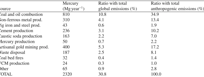
Table 2. Global mercury emissions from anthropogenic sources (reproduced from Pirrone et al. [57]).

Mercury Ratio with total Ratio with total

Source (Mg year−1_{) global emissions (%) anthropogenic emissions (%)}

Coal and oil combustion 810 10.8 34.9

Non-ferrous metal prod. 310 4.1 13.4

Pig iron and steel prod. 43 0.6 1.9

Cement production 236 3.1 10.2

Caustic soda production 163 2.2 7.0

Mercury production 50 0.7 2.2

Artisanal gold mining prod. 400 5.3 17.2

Waste disposal 187 2.5 8.1

Coal bed fires 32 0.4 1.4

VCM production 24 0.3 1.0

Other 65 0.9 2.8

TOTAL 2320 30.8 100.0

since the Industrial Age, primarily as a consequence of anthropogenic activities [78]. Today, tens of thousands of uncontrolled coal fires are active in the world, which emit mercury among other com-pounds [79]. The amount of mercury released annually to the atmosphere by uncontrolled coal-bed fires is 32 Mg (1% of total anthropogenic emissions).

3.2.9 Vinyl chloride monomer production

Vinyl chloride monomer (VCM) is an intermediate feedstock in the production of polyvinyl chloride (PVC), which production process uses sometimes mercuric chloride on carbon pellets as a catalyst. Mercury emissions have been estimated from global production of PVC [57], showing 24 Mg of mer-cury annually released to the atmosphere.

3.2.10 Global assessment form anthropogenic emissions

Summing up the contributions from anthropogenic sources, nearly 2320 Mg of mercury is released annually to the global atmosphere (31% of total global emissions) Table 2. The present assessment shows that the majority of mercury emissions originate from combustion of fossil fuels (11%), followed by artisanal small scale gold mining (5%), non-ferrous metal production (4%), cement pro-duction (3%), caustic soda propro-duction (2%), waste incineration (2%) and pig-iron propro-duction (1%). In the last decades a considerable amount of research has been done to improve mercury emission inventories at country level, including those countries with economies in transition [73, 80]. Recent estimates show that Europe and North America are reducing their contribution to the global mercury burden, whereas emissions in Asia are increasing, the latter is primarily driven by the upward trend of energy demand that in the last decade has grown at a rate of 6 to 10% per year Figure 2.

3.2.11 Trend in global emissions

AF 9%

AS 38% OC

3% EU

33% _14%NA

SA 3%

1990

AF 11% AS

56% OC

6% EU

13% _NA

11%

SA 3%

1995

AF 18% AS

55%

OC

6% EU

11% _NA

6% SA 4%

2000

AF 2%

AS 64% OC

1% 14%EU NA_9%

SA 10%

2007

[a] [b]

[c] [d]

Fig. 2. Trends of global anthropogenic emissions by region based on (a) Pirrone et al. [1], (b) Pacyna et al. [46], (c)

Pacyna et al. [5], (d) Pirrone et al. [57]. Data reported in Fig. 2(d) are for most contributing countries as reported in Pirrone et al., [57]. AF, Africa; AS, Asia; EU, Europe; NA, North America; OC, Oceania; SA, South America. Reproduced from Pirrone et al. [57].

Table 3. Comparison of mercury emissions (Mg year−1_{) as reported in the literature (reproduced from Pirrone}

et al., [81]).

Reference year 1985 1990 1995 20001 2006 2000/2005 2005 2000/2005 2005 Anthropogenic

emissions

1989 2217 2427 2254 18942 2501 1926 2909 2320

Reference [1] [1] [46] [5] [15] [27] [6] [2] [57]

Reference year 1999 2002 2002 2004 2007 2008 2008 Natural emissions 5300 4200 3600 4278 4800 4532 5207 Reference [180] [34] [40] [181] [182] [4] [57]

1_{Updated with Pacyna et al. [5];}2_{Without considering biomass burning; the estimate is based on}

emitting sectors instead of source categories.

3.2.12 Uncertainty of assessments

4 Spatial distribution of mercury species in the atmosphere

Long-term atmospheric Hg monitoring and additional ground-sites are important in order to provide datasets which can give new insights and information about the worldwide trends of atmospheric Hg. A successful Hg monitoring network, would need to consist of a relatively small number of “intensive” sites, where the full range of measurements are made (i.e., Hg speciation in ambient air and dry deposition estimation, event-based wet deposition and fluxes, as well as ancillary parameters and detailed meteorology), and a larger number of “cluster” sites where only weekly wet deposition sam-ples are collected. The cluster sites would allow for integration between the intensive sites and examine the effects of local and regional conditions, while the intensive sites would provide the detailed infor-mation needed to calibrate and test global and regional Hg models. Existing measurement networks are however not sufficient because of the lack of (a) observations of all forms of Hg in ambient air and in both wet and dry deposition; (b) co-located long-term measurements of Hg and other air pollutants; (c) representation of sites in the free-troposphere of both Southern and Northern Hemisphere; and (d) measurement sites that allow a careful investigation of inter-hemispheric transport and trends in background concentrations. Mercury concentration measurements in ambient air of documented and accepted quality are available from the mid 1970s and the mid 1990s for the Northern and Southern Hemispheres, respectively.

4.1 Mercury measurements in Europe

4.2 Hg measurements and air/water exchange over Atlantic, Pacific and Arctic Oceans

was overestimated due to the fjord being partly ice covered, thus, hindering the wave field. St. Louis et al. [105] carried out measurements of DGM at two ice-covered locations offof Ellesmere Island and found average concentrations of 129±36 pg L−1_{, which corresponds to super-saturation conditions.} The average flux calculated according to Wanninkhof and McGillis [106] was 5.4±1.2 ng m−2_hr−1 on average; higher fluxes would be expected during Hg depletion events and ice-breakup and melting in the Spring. Andersson et al. [107] carried out continuous measurements of DGM over the Arctic Ocean. Measurements were carried out in both ice-covered and non ice-covered areas, and the DGM concentration increased up to 80% between non-ice-covered and ice-covered areas. During the transit through ice-covered areas, enhanced TGM concentrations were observed which were expected to be higher when the ship breaks the ice layer. An Hg(0) evasion flux of 98 ng m−2hour−1was estimated. During summer 2005 (July - September), a cruise was performed over the Atlantic and Arctic Oceans from 60◦ to 90◦N [108]. The results reported by Sommar et al. [108] have highlighted that higher TGM/Hg(0) concentrations were observed during Arctic summer over the ice-capped sea. However, a rapid increase of TGM/Hg(0) in air and surface water were observed when the Swedish icebreaker Oden went from the North Atlantic into the ice-covered waters of the Canadian Arctic archipelago. Higher Hg(0) levels were, in fact, obtained along the sea-ice route (1.81±0.43 ng m−3_{) compared to} those observed in the MBL over ice-free oceanic waters (1.55±0.21 ng m−3_).

4.3 Hg measurements and air/water exchange over European seas

4.3.1 Mediterranean

An in-depth investigation was carried out from 2000 to 2007 by several research groups in the frame-work of the MED-OCEANOR project [24, 87, 109, 110] to quantify and possibly explain spatial and temporal patterns of Hg species concentrations in air, surface and deep water samples, and gaseous Hg exchange rates at the air-water interface over the Mediterranean Sea [24, 87, 89, 109, 111–113]. The sampling campaigns were performed during different seasons and covered both the western and east-ern sectors of the Mediterranean basin. A summary of the overwater Hg species observed during the Mediterranean cruises can be found in Table 4. Observations of the Hg evasion by Ferrara et al. [3] over the Tyrrhenian Sea during 1998 showed a typical daily trend suggesting that solar radiation is one of the major driving factors affecting the release of Hg(0) from surface waters. In addition, a seasonal trend was also observed, with minimum values during the winter period and maximum values during the summer, probably due to the higher water temperature that may have facilitated biotic and abiotic processes involving Hg in the water column. The average Hg evasion value estimated for the western Mediterranean Sea was lower than the eastern sector, probably due to the higher mean degree of Hg(0) saturation in the east compared to the west [112]. Past or present tectonic activity may contribute to the high DGM concentrations found in these areas, enhancing higher Hg evasions from the seawa-ter [112]. The Hg(0) evasion reported by Gårdfeldt et al. [111] from the wesseawa-tern Mediseawa-terranean and the Tyrrhenian Sea is of the same order of magnitude as that estimated by both Ferrara et al. [3] and Cossa et al. [114]. DGM data combined with a gas-exchange model [103] suggested that about 66 tonnes of Hg(0) are released into the atmosphere from the Mediterranean Sea during the summer. This emission estimate is comparable with the amount ofHg emitted from stationary combustion facilities in Europe [57].

4.3.2 North sea

4.3.3 Baltic sea

Six expeditions have been carried out in the Baltic Sea. Wangberg et al. [117] conducted two of these in summer 1997 and winter 1998 in the southern area. Higher flux (1.6 ng m−2_hour−1_{), calculated} using the Wanninkhof [103] model was estimated for the summer, whereas the winter estimate was much lower (0.8 ng m−2_hour−1_{). In 2006, Kuss and Schneider [118] carried out continuous} measure-ments in the southern Baltic Sea during all seasons. The lowest DGM concentrations were measured during winter and autumn (10–17 pg L−1 and 11–14 pg L−1, respectively), whereas the highest con-centrations were observed during summer (ranging between 19–32 pg L−1_{) and spring (between 15–} 20 pg L−1_{). The lowest flux, calculated using the Weiss et al. [119] model, was estimated to occur} during the winter season (from−0.2 to 0.2 ng m−2_hour−1_{), whereas the highest was in the summer} (between 3.1 and 6.2 ng m−2hour−1). During the spring and autumn expeditions, fluxes were ranging between 1.0–2.1 and 0.8–2.1 ng m−2_hour−1_{, respectively. On the basis of estimated flux evasion and} deposition rates, mass balance was not achieved for the Baltic Sea suggesting that key sources, primary and secondary, have not been accounted for.

4.4 Mercury measurements in North and South America

up to 16 ng m−3 _{[122]. Higueras et al. [123] observed very high TGM concentrations near historical} mining regions in the Coquimbo region of Northern Chile, reaching extremely high TGM values, up to 100µg m−3_{at some gold recovery operations. Fostier and Michelazzo [124] performed TGM} measure-ments at two sites in Sao Paulo State, Brazil, near an industrial area. An average TGM concentration up to global background (7.0 ng m−3) was observed at both sites due to a wide array of industrial sources in the area. Higher TGM concentrations (mean 15.0 ng m−3_{) were also found by Amouroux} et al. [125] at several sites in French Guiana strongly influenced by mining activities along with illegal gold mining. It is clear that past and current gold mining activities in South America represent a large source of Hg entering into the atmosphere. While emissions of Hg from gold mining in South Amer-ica are clearly a substantial source to the global atmosphere, there is a signifAmer-icant uncertainty in the current estimate. TGM concentrations have been performed by De La Rosa et al. [126] during short-term sampling campaigns at 4 sites in 2002 (two urban/industrial cities, Mexico City and Zacatecas, and two rural/remote sities, Puerto Angel and Huejutla). High variability in TGM levels were found between these sites suggesting a strong influence of local sources. In particular, at Zacatecas, though it is a smaller semi-urban centre compared to Mexico City, but with a history of gold and silver mining activities, the mean Hg values were very high at 71.7 ng m−3_{. At Mexico City, mean TGM values were} found to be 34 ng m−3_{, whereas at the two rural/remote sites mean TGM concentrations were close to} hemispheric background concentrations (1.46 and 1.32 ng m−3_).

4.5 Mercury measurements in Asia

these values are, however, much lower than semi-rural and industrial/urban areas, indicating signif-icant emissions of Hg in central, south and southwest China. Feng et al. [132] have reported TGM concentration data for Guiyang city in 2001 with a mean value of 8.40 ng m−3 _{on the basis of one} year of observations (from November 2001 to November 2002). The average TGM concentration in ambient air observed in Guiyang in 1996 and 1999 was 11 ng m−3and 13 ng m−3, respectively [132]. The authors concluded that TGM concentrations in Guiyang are significantly elevated compared to the continental global background values and that coal combustion from both industrial and domestic use is probably the primary atmospheric source. Similar data were obtained earlier ([133] during 4 measurement campaigns in 2000 and 2001 in Guiyang. Significant Hg emissions from anthropogenic sources resulted in high levels of atmospheric Hg also in Guizhou [134]. Hg species as well as haz-ardous heavy metals in particles and in precipitation have been continuously measured from 2007 at Cape Hedo Atmosphere and Aerosol Monitoring Station (CHAAMS) located on the north end of the island of Okinawa, Japan. This monitoring station has been used for many years to study the outflow of pollution from China and East Asia [39]. Monthly mean concentrations of Hg(0) from October 2007 to January 2008 (UNEP/ABC (Atmospheric Brown Clouds) project) were approximately 1.3 to 1.7 ng m−3_{, which were slightly lower than the spring observation in 2004 (2.04 ng m}−3_{) [39].}

4.6 Mercury measurements in Africa

Observations from Cape Point (South Africa) constitute the only long-term dataset of atmospheric TGM in the Southern Hemisphere. The monitoring of TGM was established at the Cape Point Global Atmospheric Watch (GAW) station in September 1995. Baker et al. [97] presented data of atmospheric Hg covering the period from the start of the measurements (September 1995) until June 1999. Atmospheric Hg concentrations were found to be fairly homogeneous over time ranging between 1.2–1.4 ng m−3_{. Whilst no significant diurnal variation was detectable, a slight seasonal variation with} a TGM minimum in springtime and maximum in summertime was observed. The most prominent feature of the highly resolved TGM data is the frequent occurrence of events with almost complete mercury depletion which has so far not been observed at any other non-polar stations [28].

4.7 Mercury measurements at high altitude locations (including aircraftmeasurements)

recent studies, TGM and CO were measured in 22 pollution transport “events” at Mt. Bachelor (2800 m asl) between 2004 and 2005 [138]. East Asian outflow events yielded a TGM/CO enhancement ratio of about 0.005 ng m−3_ppbv−1_{, whereas plumes from western USA anthropogenic sources and from} biomass burning in the Pacific Northwest and Alaska gave a ratio of about 0.001 ng m−3_ppbv−1_{. The} TGM/CO ratio is therefore, an important distinguishing feature to identify Asian long-range transport patterns. Scaling these ratios with estimated emissions of CO from China and global biomass burning, an emission of 620 Mg year−1_{is calculated for total Hg emissions from Chinese anthropogenic sources} and 670 Mg year−1_{for global biomass burning. The Hg(0)/CO molar enhancement ratio was observed} in pollution plumes at Cape Hedo Station, Okinawa, Japan which is nearly twice the expected ratio based on emissions estimates from China [39]. These plumes originated from the industrialized region of eastern China and produced a similar ratio to those observed at Mt. Bachelor, highlighting the dis-crepancy between the results observed and the recent Chinese emission inventories. These findings are probably due to large natural sources of Hg not accounted for and/or underestimated Hg emissions. The first reported data on Hg species performed at high altitude are from Mauna Loa, (Hawaii Moni-toring Site, [140] and Mt. Bachelor, (Oregon, USA, [143]. Both sites revealed elevated Hg(II) values in the free troposphere (about 350 pg m−3_{at Mauna Loa and about 600 pg m}−3_{at Mt. Bachelor),} reach-ing those of the most polluted urban environments. Several high Hg(II) events, generally accompanied by a decrease in Hg(0), have been observed under meteorological conditions clearly marked by dry (free tropospheric) air at night [143]. Swartzendruber et al. [143] observed that the mean Hg(II) con-centration at night was 60 pg m−3_{, whereas the daytime mean value was 39 pg m}−3_{in contrast to other} studies showing an Hg(II) maximum at solar noon. Hg(P) concentrations were equivalent for day and night (about 4.4 pg m−3_{). This implies that Hg(II) formed in situ was unable to condense to particles} under these dry air conditions. Both these studies ([140, 143] found very similar observations point-ing out that the high Hg(II) concentrations observed, first in Hawaii and later in Oregon were due to atmospheric oxidation and not related to pollution events. Similar results have been obtained in Col-orado at the Storm Peak Laboratory high altitude research station (3220 m asl) by Fa¨ın et al. [7]. They showed a very regular occurrence of high Hg(II) levels in dry tropospheric air that was not related to pollution events, but highlighted signs of atmospheric oxidation, likely in the free troposphere, and possibly over the Pacific Ocean. These observations provide evidence that the free tropospheric pool of Hg is enriched with Hg(II) compared to the boundary layer where high Hg(II) levels are mainly related to local and regional pollution.

4.8 Mercury measurements in Arctic and Antarctic Regions

following polar sunrise. During these events, Hg(0) may be converted to Hg(II) and/or Hg(P), that deposit quickly into the snow/ice pack increasing the mercury deposition fluxes considerably. Springtime AMDEs have also been observed in Antarctica [16]. AMDEs occur at the same time as tropospheric ozone depletion events (ODEs) suggesting that both species were removed by similar chemical mechanisms involving reactive halogen species (i.e., Br and BrO) across open waters and polynas. BrO is one of the species observed during ODEs and, therefore, often used as an indicator for such events. Several experiments have been performed at different Arctic and sub-Arctic locations (Ny-Ålesund, Svalbard 78◦54’N 11◦53’E [145, 146, 151, 152]; Pt. Barrow, Alaska 71◦19’N 156◦37’W [153]; Station Nord, Greenland 81◦36’N 16◦40’E [154]; Kuujjuarapik, Quebec 55◦16’N 77◦45’W [155]; Amderma, Russia 69◦45’N 61◦40’E [156]. While the tropospheric reactivity of mercury in the Arctic is more and more documented only a few attempts were made to study the Hg cycle in Antarc-tica. AMDEs were observed in Coastal Antarctica after polar sunrise at Neumayer and Terra Nova Bay [144, 157]. The study of the Hg cycling in Antarctica is first necessary to understand and follow the extent of the contamination within these ecosystems. Mercury concentrations in biota of some Arctic areas are known to have increased with time [158] and to be rather high. In Antarctica, available data on Hg concentrations in water, sediments, phytoplankton, macroalgae, krill and several species of ben-thic invertebrates compiled by Bargagli et al. [159] indicate that there is no enhanced bioavailability of Hg in the Southern Ocean food web. However, recent studies showed an enhanced Hg bioaccumu-lation in terrestrial ecosystem samples collected close to Terra Nova Bay [160], suggesting that local deposition events of Hg may impact these ecosystems. Mercury measurements performed at different locations within the Arctic and Antarctic regions are reported in Table 5, which is from Dommergue et al. [149] The first extended baseline data for the concentration and speciation of atmospheric Hg in Antarctica were reported by De Mora et al. [161]. The measurements reported by Ebinghaus et al. [16] comprise of the first annual time series of ground-level TGM concentrations in Antarctica to investi-gate the occurrence of possible AMDEs in south polar regions. The study also provides high-resolution data that can be compared with existing datasets of AMDEs in the Arctic, and reveals similarities. The TGM series measured at Neumayer showed several Hg depletion events during Antarctic springtime (between August and November 2000); TGM and O3were strongly and positively correlated as seen in the Arctic boundary layer after polar sunrise. Simultaneous measurements of Hg(0) and Hg(II) were performed at Terra Nova Bay from November 2000 to January 2001. ODEs and MDEs were not observed throughout this period at Terra Nova Bay, however, Hg(II) concentrations during the mea-surement period were surprisingly high and comparable with those at sites directly influenced by significant anthropogenic Hg sources suggesting that there are specific mechanisms and/or charac-teristics of polar environments that at certain times, and apparently in the presence of surface snow, are extremely favourable to the production of Hg(II). Comparable Hg(II) results have been reported by Temme et al. [147] at Neumayer during Antarctic summertime suggesting that the snow-pack is directly involved in maintaining high Hg(II) concentrations. Long-term measurements of Hg(0) and other atmospheric Hg species in the Polar Regions are very limited and need to be increased. These types of measurements can yield critical information for a better understanding of the processes in-volved in the Hg cycle in the polar atmosphere and the mechanisms characterizing the deposition of this pollutant to this fragile environment.

5 Chemical and physical processes affecting atmospheric mercury

atmospheric transport. Mercury can be oxidised and reduced in the gas phase and the aqueous phase. It can also undergo reaction at air/snow and air/water surfaces air/solid although most of the studies of these heterogeneous have been at terrestrial or marine interfaces, or under conditions representa-tive of flue gases in the latter instance. It is not clear whether the same reactions seen at the surface would occur on a droplet or snowflake in the atmosphere. This discussion will be limited therefore primarily to homogeneous reactions. The atmospheric oxidants generally considered to be the most important in terms of Hg oxidation are O3, OH and Br. Experimental determinations of the reaction rate constants for these oxidants at conditions similar to those of the atmosphere (troposphere in par-ticular) have proved to be difficult. There is still some debate over whether some of them, O3 and OH, actually oxidise Hg at all in the atmosphere, [162] and thus there has been some questioning of the experimental techniques used in the determination of the reaction rate constants [30]. A detailed review of the methods and a comparison of the results obtained from the various laboratory, theo-retical and field determination of Hg reaction kinetics can be found in Hynes et al. and Ariya et al. [30, 163]. The one reaction which is unanimously accepted is the reaction of Hg with Br. This reaction is responsible for the Hg depletion events first observed in the Arctic around polar dawn [150]. The depletion of Hg occurs at the same time as O3 is destroyed, thereby eliminating both O3 and OH as potential candidates for the observed decrease in Hg(0) concentration leaving Br as the only known candidate. A box modelling study using the observed O3 decrease to constrain the Br concentration showed that the published rate constants for Hg+Br, both experimental [164] and theoretical [165], managed to reproduce the observed decrease in Hg(0) concentration [166]. The reaction of Hg with Br has been examined in global and regional modelling contexts, [166–169]. It appears that the re-actions of Hg with O3and OH are not necessary to explain a number of the major features of Hg(0) and Hg(II) concentration fields in the atmosphere. There is an important caveat to the above state-ment however. It is possible that reduction reactions are occurring in the gas phase in the atmosphere. Two suggestions have been made in the literature, one is CO, which is known to reduce solid Hg(O), [170] although experiments under conditions which resemble those in the atmosphere have not as far as we are aware been performed. The other is SO2, the evidence that this reaction may be taking place comes from modelling studies of power plant plumes and was suggested by Vijayaraghavan et al. [171]. Reduction processes are extremely important in the overall Hg cycle, it is the reduction of deposited Hg(II) on land and sea surfaces which permits the re-emission of Hg(0) and ensures that it is transported all round the globe. Currently the known reduction reactions for atmospheric Hg occur in the atmospheric aqueous phase. Oxidation also occurs in the aqueous phase, however in comparison to gas phase oxidation it contributes very little to the overall Hg(II) atmospheric concen-tration. In the atmospheric aqueous phase Hg(II) can form coordination complexes with SO2₃−, to give HgSO3 and Hg(SO3)2₂−, the latter is redox stable while the former is not, and HgSO3can dissociate in the presence of water to give Hg(0)+SO−₄ +H+. The other reduction which has been identified in the laboratory, but whose atmospheric relevance is debated, is the reaction of Hg(II) with HO2. The reduction to Hg(0) is a two step process, Hg(II) reacting with HO2 to give Hg(I) which is then further reduced by another HO2. The point which some authors have called into question (see Gård-feldt et al. [172]) is the reduction of Hg(I), as they assert that Hg(I) in the presence of dissolved O2 would be extremely rapidly re-oxidised back Hg(II), thereby competing with the second reduction step and blocking the production of Hg(0). The lack of certainty over the basic atmospheric chemistry of Hg leads to uncertainty in the atmospheric modelling of Hg, which in turn produces uncertain-ties in estimates of Hg deposition fluxes and limits our ability to determine the possible influences of changes in Hg emissions or the response of the atmospheric part of the Hg cycle to climate change forcing.

5.1 Atmospheric mercury modelling

models to better understand air/sea interactions in the global Hg atmospheric cycle. Regional mod-elling of Hg emission, transport and chemistry has been the subject of a number of review articles over the last few years [170, 173–176], and although they have improved over the years they suffer form limitations in the representation of atmospheric Hg chemistry, and are plagued by the fact that they are very susceptible to the boundary conditions which are employed. Pongprueksa et al, [170] demonstrated with the CMAQ-Hg model, that the response of the modelled Hg concentration and de-position to changes in the boundary conditions used was nearly linear (r2 _{= 0.99) with a 1 ng m}−3 increase in BC Hg(0) concentration producing an increase of 0.81 ng m−3_{in the average model Hg(0)} concentration. The response to initial conditions was similar but weaker a 0.14 ng m−3increase in the average model Hg(0) concentration for a 1 ng m−3increase in the initial Hg(0) condition. For this rea-son over recent years a lot of effort has been made to improve global Hg models as it is now clear that they are required to provide the boundary conditions for regional models if the regional model output is to be credible. An overview of most of the models used to simulate global atmospheric Hg chemistry can be found in the recent Mercury Fate and Transport Report to UNEP (Chapters 17–21), [177]. Most of these models have used the Hg +O3/OH oxidation scheme and the HO2 reduction of Hg(II) in the aqueous phase as the basis of their atmospheric Hg scheme up to now. In the last couple of years however the focus of modelling studies has been moving away from this almost ‘tradi-tional’ approach in an attempt to determine the role of Br in atmospheric Hg chemistry. These include box modelling studies of the role of the Hg+Br in the Arctic [166], and also the Marine Boundary Layer in the Mediterranean [89, 169] and the remote Pacific and Atlantic [168]. This new focus also includes an investigation of Hg chemistry in volcanic plumes using a one-dimensional model, [178], and an investigation into the global free tropospheric lifetime of Hg(0) atmospheric Hg against oxida-tion by Br [167]. Most recently a global model has been used to investigate the relative merits of the O3/OH oxidation scheme in comparison to the Br oxidation scheme [179]. It appears to the authors that consensus is coming down on the side of Bromine as the major Hg oxidant in the atmosphere. This will cause a number of problems for modellers because while O3precursor emission chemistry and OH production are relatively well known, Br emission sources are less well characterised and introducing Br chemistry into current atmospheric chemistry models could prove to difficult. It should be pointed out that while it seems that the question of atmospheric Hg oxidation may be being re-solved, that of atmospheric Hg reduction does not. Almost all modelling studies suffer from a lack of long term Hg concentration and flux data with which to compare their output. While some series exist for parts of Europe and North America they are the exception, and the Southern hemisphere in particular has an extremely sparse data set with which models can be compared. This is a situa-tion which given some of the serious uncertainties inherent in current models really does need to be rectified.

6 Major policy frameworks

the release of mercury and its compounds improving global understanding of international mercury emission sources, fate and transport. In this framework, the UNEP Global Partnership for Mercury Air Transport and Fate Research (UNEP-MFTP) was started in 2005 aiming to encourage collabora-tive research activities on different aspects of atmospheric mercury cycling on local to hemispheric and global scales. Recently, as part of the work plan (2009-2011) of the Group on Earth Observations (GEO), the Task 09-02d “Global Monitoring Plan for Atmospheric Mercury” aiming to develop a global observation system for mercury was established. This task supports the achievement of the goals of GEOSS and other on-going international programs (e.g. UNEP Mercury Program) and conventions (i.e., UNECE-LRTAP TF HTAP). Programs such as the World Meteorological Organization’s Global Atmosphere Watch (GAW) have made substantial efforts to establish data centres and quality con-trol programs to enhance integration of air quality measurements from different national and regional networks, and to establish observational sites in under-sampled, remote regions around the world. Similarly, the International Global Atmospheric Chemistry project (of the International Geosphere-Biosphere Programme) has strongly endorsed the need for international exchange of calibration stan-dards, and has helped coordinate multinational field campaigns to address a variety of important issues related to global air quality. Following the lead of these programs, the incorporation of a well-defined Hg monitoring component into the existing network of sites would be the most expeditious and effi-cient approach to realise a global Hg monitoring network. Close coordination of the global modelling community with the global measurement community would lead to major advances in the global mod-els, and also advance our understanding of Hg science, while at the same time decreasing the uncer-tainties in global assessments for Hg entering aquatic and terrestrial ecosystems.

References

1. N. Pirrone, G.J. Keeler, J.O. Nriagu, Atmospheric Environment 30(17), 2981 (1996)

2. N. Pirrone, S. Cinnirella, X. Feng, R.B. Finkelman, H.R. Friedli, J. Leaner, R. Mason, A.B. Mukherjee, G. Stracher, D.G. Streets et al., in Mercury Fate and Transport in the

Global Atmosphere: Emissions, Measurements and Models, edited by N. Pirrone, R.P. Mason

(Springer, 2009), chap. 1, pp. 1–47

3. R. Ferrara, B. Mazzolai, E. Lanzillotta, E. Nucaro, N. Pirrone, The Science of The Total Environment 259(1–3), 183 (2000)

4. R.P. Mason, in Mercury Fate and Transport in the Global Atmosphere: Emissions, Measurements

and Models, edited by N. Pirrone, R.P. Mason (Springer, 2009), chap. 7, pp. 173–191

5. E.G. Pacyna, J.M. Pacyna, F. Steenhuisen, S. Wilson, Atmospheric Environment 40(22), 4048 (2006)

6. E. Pacyna, J. Pacyna, K. Sundseth, J. Munthe, K. Kindbom, S. Wilson, F. Steenhuisen, P. Maxson, Atmospheric Environment 44(20), 2487 (2010)

7. X. Fa¨ın, D. Obrist, A.G. Hallar, I. Mccubbin, T. Rahn, Atmospheric Chemistry and Physics 9(20), 8049 (2009)

8. P. Weiss-Penzias, D.A. Jaffe, P. Swartzendruber, J.B. Dennison, D. Chand, W. Hafner, E. Prestbo, Journal Of Geophysical Research - Atmospheres 111(D10), D10304 (2006)

9. S. Lindberg, R. Bullock, R. Ebinghaus, D. Engstrom, X. Feng, W. Fitzgerald, N. Pirrone, E. Prestbo, C. Seigneur, AMBIO: A Journal of the Human Environment 36(1), 19 (2007) 10. D.M. Murphy, P.K. Hudson, D.S. Thomson, P.J. Sheridan, J.C. Wilson, Environmental Science

& Technology 40(10), 3163 (2006)

11. R. Talbot, H. Mao, E. Scheuer, J. Dibb, M. Avery, Geophys. Res. Lett. 34(23), L23804 (2007) 12. N. Pirrone, I. Allegrini, G.J. Keeler, J.O. Nriagu, R. Rossmann, J.A. Robbins, Atmospheric

En-vironment 32(5), 929 (1998)

13. R. Bindler, I. Renberg, P.G. Appleby, N.J. Anderson, N.L. Rose, Environmental Science & Technology 35(9), 1736 (2001)

14. H. Biester, R. Kilian, C. Franzen, C. Woda, A. Mangini, H.F. Sch¨oler, Earth and Planetary Science Letters 201, 609 (2002)

16. R. Ebinghaus, H.H. Kock, A.M. Coggins, T.G. Spain, S.G. Jennings, C. Temme, Atmospheric Environment 36(34), 5267 (2002)

17. F. Slemr, R. Ebinghaus, P. Simmonds, S. Jennings, Atmospheric Environment 40(36), 6966 (2006)

18. W.F. Fitzgerald, Water, Air, & Soil Pollution 80(1), 245 (1995)

19. K.H. Kim, R. Ebinghaus, W.H. Schroeder, P. Blanchard, H.H. Kock, A. Steffen, F.A. Froude, M.Y. Kim, S. Hong, J.H. Kim, Journal of Atmospheric Chemistry 50(1), 1 (2005)

20. N. Pirrone, P. Costa, J.M. Pacyna, R. Ferrara, Atmospheric Environment 35(17), 2997 (2001) 21. I. W¨angberg, J. Munthe, N. Pirrone, A. Iverfeldt, E. Bahlman, P. Costa, R. Ebinghaus, X. Feng,

R. Ferrara, K. Gårdfeldt et al., Atmospheric Environment 35(17), 3019 (2001)

22. I. W¨angberg, J. Munthe, D. Amouroux, M. Andersson, V. Fajon, R. Ferrara, K. Gårdfeldt, M. Horvat, Y. Mamane, E. Melamed et al., Environmental Fluid Mechanics 8(2), 101 (2008) 23. J. Munthe, I. W¨angberg, N. Pirrone, Å. Iverfeldt, R. Ferrara, R. Ebinghaus, X. Feng, K.

Gårdfeldt, G. Keeler, E. Lanzillotta et al., Atmospheric Environment 35(17), 3007 (2001) 24. N. Pirrone, M. Wichmann-Fiebig, Atmospheric Environment 37

(Supplement 1), 3 (2003)

25. N. Pirrone, Atmospheric Environment 35(17), 2979 (2001)

26. I.M. Hedgecock, N. Pirrone, Environmental Science & Technology 38(1), 69 (2004) 27. N. Pirrone, I.M. Hedgecock, F. Sprovieri, Atmosperic Environment 42(36), 8549 (2008) 28. E.G. Brunke, C. Labuschagne, R. Ebinghaus, H.H. Kock, F. Slemr, Atmospheric Chemistry and

Physics 10(3), 1121 (2010)

29. F. Sprovieri, N. Pirrone, R.P. Mason, M. Andersson, in Mercury Fate and Transport in the Global

Atmosphere: Emissions, Measurements and Models, edited by N. Pirrone, R.P. Mason (Springer,

2009), chap. 11, pp. 323–380

30. A.J. Hynes, D.L. Donohoue, M.E. Goodsite, I.M. Hedgecock, in Mercury Fate and Transport in

the Global Atmosphere: Emissions, Measurements and Models, edited by N. Pirrone, R.P. Mason

(Springer, 2009), chap. 14, pp. 427–457

31. N.E. Selin, Annual Review of Environment and Resources 34(1), 43 (2009) 32. E.M. Sunderland, R.P. Mason, Global Biogeochem. Cycles 21(4), GB4022 (2007)

33. N.E. Selin, D.J. Jacob, R.M. Yantosca, S. Strode, L. Jaegl´e, E.M. Sunderland, Global Biogeochem. Cycles 22, GB2011 (2008)

34. R.P. Mason, G.R. Sheu, Global Biogeochem. Cycles 16(4), 1093 (2002)

35. S.A. Strode, L. Jaegl´e, N.E. Selin, D.J. Jacob, R.J. Park, R.M. Yantosca, R.P. Mason, F. Slemr, Global Biogeochem. Cycles 21(1), GB1017 (2007)

36. J.F. Hamilton, G. Allen, N.M. Watson, J.D. Lee, J.E. Saxton, A.C. Lewis, G. Vaughan, K.N. Bower, M.J. Flynn, J. Crosier et al., Journal Of Geophysical Research - Atmospheres 113(D20), D20313 (2008)

37. I. W¨angberg, J. Munthe, T. Berg, R. Ebinghaus, H. Kock, C. Temme, E. Bieber, T. Spain, A. Stolk, Atmospheric Environment 41(12), 2612 (2007), ISSN 1352-2310

38. Å. Iverfeldt, J. Munthe, C. Brosset, J. Pacyna, Water, Air, & Soil Pollution 80(1), 227 (1995) 39. D. Jaffe, E. Prestbo, P. Swartzendruber, P. Weiss-Penzias, S. Kato, A. Takami, S. Hatakeyama,

Y. Kajii, Atmospheric Environment 39(17), 3029 (2005)

40. C.H. Lamborg, W.F. Fitzgerald, A.W.H. Damman, J.M. Benoit, P.H. Balcom, D.R. Engstrom, Global Biogeochem. Cycles 16(4), 1104 (2002)

41. J. Munthe, R.A.D. Bodaly, B.A. Branfireun, C.T. Driscoll, C.C. Gilmour, R. Harris, M. Horvat, M. Lucotte, O. Malm, AMBIO: A Journal of the Human Environment 36(1), 33 (2007)

42. C.D. Knightes, E.M. Sunderland, M.C. Barber, J.M. Johnston, R.B. Ambrose, Environmental Toxicology and Chemistry 28(4), 881 (2009)

43. D.M. Orihel, M.J. Paterson, P.J. Blanchfield, R.A.D. Bodaly, H. Hintelmann, Environmental Science & Technology 41(14), 4952 (2007)

44. H. Hintelmann, R. Harris, A. Heyes, J.P. Hurley, C.A. Kelly, D.P. Krabbenhoft, S. Lindberg, J.W.M. Rudd, K.J. Scott, V.L. St. Louis, Environmental Science & Technology 36(23), 5034 (2002)