Markets for non-storable commodities

VICTORIA ~ UNIVERSITY

•

~

₀

0 0

..

DEPARTMENT OF COMPUTER AND

MATHEMATICAL SCIENCES

Markets For Non-Storable Commodities

Barry A. Goss and S. Gulay A vsar

•

83 ECON7

April, 1997

(AMS

: 90A58, 62J99)

TECHNICAL REPORT

VICTORIA UNIVERSITY OF TECHNOLOGY

P OBOX 14428

MELBOURNE CITY MC

VIC 8001

AUSTRALIA

TELEPHONE (03) 9688 4492

FACSIMILE (03) 9688 4050

MARKETS FOR NON-STORABLE COMMODITIES

by

BARRY

A. Goss

AND

s.

GULA y A

VSAR*

Revised September 1996

MARKETS FOR NON-STORABLE COMMODI'l'IES

by

BARRY

A.

Goss A~D

s.

GULA y

A

VSAR*

ABSTRACT

Published empirical studies of simultaneous rational expectations models of spot and futures markets for non-storable commodities, such as finished live cattle, are extremely rare. Indeed, only two countries, the US and Australia, have produced data sets for the study of such markets. This paper develops, and presents estimates of a simultaneous rational expectations model of the live cattle market in Australia, the world's leading beef exporting country. The model contains functional relationships for short hedgers and speculators combined (there is no disaggregation of hedgers' and speculators' commitments in Australian data), long hedgers and speculators, and consumers, and is completed with a spot price equation and market clearing identity. Augmented Dickey-Fuller and Phillips-Perron tests for unit roots yield ambiguous results, but the Phillips-Perron tests, taken as definitive, indicate that several variables are I(l), including spot and futures prices, real income and consumption of beef, the others being stationary. Johansen cointegration tests indicate that where two or more I(l) variables appear in a structural equation, they are cointegrated. Structural equations with rational expectations are estimated by the instrumental variables method of McCall um in the absence of serial correlation, and by non-linear least squares when a correction for autocorrelation is required. The estimates of all 15 structural parameters have the expected sign, and all are significant at the five per cent level. In a 34 month post-sample period, the model forecasts consumption with a per cent RMSE of 2.3% and spot and futures prices with per cent RMSE's of 4.6% and 2.8% respectively. In forecasting the spot price, the model outperforms, but not significantly, conventional benchmarks such as a random walk, an ARIMA model, and a lagged futures price. The outcome of this last comparison implies that the efficient markets hypothesis cannot be rejected.

JEL Codes: G13 Q13 G14

MARKETS

FOR NON-STORABLE COMMODII'IES

I

INTRODUCilON

The objective of this paper is to develop and present empirical results for a simultaneous,

rational expectations model of the Australian finished live cattle market. Finished live cattle

are non-storable, because they can be kept in their finished condition for a period -of six to

eight weeks only. This model employs information from both spot and futures markets. Only

two countries, the United States and Australia, have introduced futures contracts for live

cattle, and hence only these two countries have produced data sets for the estimation of such

models. While studies of the US live cattle market have been made, comprising simultaneous

rational expectations models, none of these studies has been published, as far as the present

authors are aware, and no such study has been made of the Australian market, to the best of

the present authors' knowledge.

Simultaneous theoretical models of the determination of spot and futures prices have

been developed by Peston and Yamey (1960), Stein (1961, 1964), Dewbre (1981) and Kawai

( 1983 ), the last of these being specifically for non-storable commodities. Empirical,

simultaneous models of (non-storable) livestock markets, without rational expectations, have

been developed and estimated by Leuthold and Hartmann (1979) and Leuthold and Garcia

(1992) and others, while empirical, simultaneous models, with rational expectations, for

storable commodities have been developed by Giles et al. (1985), Goss et al. (1992) and others. This paper extends the work of Peston and Yamey (1960), Giles et al. (1985) and

A major difference between storable and non-storable commodities, for which both

spot and futures markets exist, is that in the case of storable commodities, the extent of the

forward premium or contango (i.e. where the futures price exceeds the spot price) is limited

by the marginal net cost of storage, whereas in the case of non-storables, no such restriction

applies. (On the other hand, this restriction does not apply to the spot premium or

backwardation (i.e. where the spot price exceeds the futures price), even in the case of

storable commodities, as Keynes ( 193 0, pp. 142-44) pointed out)

International live cattle markets have attracted considerable attention from researchers,

particularly markets in the USA. Leuthold (1972) was reluctant to reject the random walk

hypothesis with US live cattle price data, even though some filter rules yielded profits net of

transaction costs. Leuthold (1974) did not reject the unbiasedness hypothesis, for US live

cattle futures prices as predictors of delivery date spot prices, with lags up to three months

I

from maturity, but did reject that hypothesis with longer lags. Giles and Goss (1980) obtained

a very similar result with Australian data. Just and Rausser (1981) compared the predictive

performance of various commercial econometric price forecasts with that of the futures price,

for a range of commodities. In the case of live cattle they found that only one commercial

forecast out of five surpassed the futures price, with a three month lag to maturity, whereas

with longer lags several commercial forecasts surpassed the futures price. While Leuthold

and Hartmann (1979) refined the model prediction approach to market efficiency (for hogs),

Leuthold and Garcia (1992) applied this approach to live cattle, and were unable to reject the

efficient markets hypothesis. The latter authors also computed the Stein (1986) social loss

measure for cattle and hogs, and found that this measure was smaller for cattle.

Australia, with 22.4 million head of cattle in 1989, is one of the leading beef

producing countries in the world, ranking behind, for example, USA (98m head), Brazil

Queensland, New South Wales and Victoria In 1989, Australia exported 872,000 tonnes of

beef, or 55.4% of production, making it the world's leading exporter of beef. The main

export markets served are in USA and Japan; indeed 76.7% of Australia's beef exports goes

to these two countries (see ABARE, 1993 ).

Although a cattle contract was introduced on the Sydney Futures Exchange in July

1975, this contract, which called for the delivery of carcases, traded thinly. Revisions were

made to this contract in May 1977, providing for the delivery of 10,000 kg live weight of

steers every calendar month (28 steers approx.). This revised contract became relatively

successful, with average monthly turnover reaching 16,559 contracts in 1981, and 28,007

contracts being traded in March of that year. By 1985, however, average monthly turnover

had fallen to 1190 contracts, and in May 1986 this Trade Steers Contract, as it had become

known, was replaced by a live cattle contract providing for mandatory cash settlement. This

last contract, although retaining I 0,000 kg live weight of cattle as the contract unit, provided

that contracts were to be settled at the Live Cattle Indicator price, which is itself an average

of cash prices for specified cattle types at specified locations. Trading in the cash settlement

contract became thin after the end of 19 8 8, and this contract was de-listed in May 1994.

The objective of this paper is to develop, present estimates of, and evaluate a

simultaneous, rational expectations model of price determination in the Australian live cattle

market. Section II of this paper discusses the specification of the model, while Section III

discusses the data employed, presents results for tests for unit roots and cointegration, and

discusses the methodology employed for estimation of the model. Results for the intra-sample

period are presented and discussed in Section IV, while Section V discusses post-sample

simulation by the model, compared with various benchmarks. Some conclusions are presented

II

MOD EL SPECIFICATION

This model contains four functional relationships and a market clearing identity. The first

equation explains the combined futures market commitments of both short hedgers and short

speculators, while the second relationship refers to the market commitments of both long

hedgers and long speculators in futures. The model contains also, a consumption relationship

and a spot price equation, and is completed with a futures market clearing identity.

This structure represents a modification of the original model by Peston and Y amey

(1960) and of the approach in the empirical models of Giles et al. (1985) and Goss et al. (1992), to deal with the case of non-storables. The combined nature of the first two equations arises because Australian futures market data on commitments of traders are not disaggregated

into hedging and speculation components, as are data for Reporting Traders provided by the

Commodity Futures Trading Commission in the USA.

Although the ideas of Working (1953, 1962) on discretionary hedging were developed for storable commodities, such as grains, his analysis of the motives for hedging is applicable

to the case of non-storables. Two of the major types of hedging distinguished by Working

(1953, 1962) are carrying charge hedging and selective hedging. On the first hypothesis, the market commitments of short hedgers, who gain from a reduction in the forward premium,

can be expected to vary directly with the current forward premium (futures price less spot

price), and negatively with the expected forward premium. If, on the other hand, short

hedgers are selective hedgers, where a proportion only of their spot market commitments is

hedged, then their futures market commitments would be expected to vary directly with the

current futures price, and negatively with the expected futures price. Preliminary estimation

for short hedgers in this market, such as beef producers, favoured the latter of these two

The market commitments of short speculators, who expect the futures price to fall can

be expected to vary directly with the current futures price, and negatively with the expected

futures price and marginal risk premium. This specification is based on the equilibrium

condition for short speculators (see Goss (1972, p. 23)). The traditional view that the

coefficient of the marginal risk premium is negative (e.g. see Kaldor (1953, p. 23) and

Brennan (1958, p. 54)), has been challenged recently by Stein (1986, pp. 48-52), who argues,

in terms of his "hedging pressure theory", that an increase in the risk premium may have a

positive or negative effect on the futures price, and hence on the market commitments of

speculators.

The supply of futures contracts by short hedgers and short speculators combined may

be expected to be a function of the sum of the influences outlined above. The specification

of this function (HSS) is therefore:

(1)

where

P

₁

=

current futures price; ,,

P,:

₁

=

rational expectation of the futures price for (t

+

I), formed in period t;

r,

= marginal risk premium;

eit

=

error term

and

e1

=

constant;

e

₂ >

o; e

₃ <

o; e-4

< >

o;

This specification suggests a predominance of speculative, rather than hedging, elements.

The rational expectations hypothesis, which is employed in this model, originated with

equation systems" and his suggestion that "rational expectations are the same as the

predictions of the relevant economic theory (Muth, 1961, p. 3 16). Much has been written on

the assumptions, implications and formation of rational expectations, and summaries of this

literature can be found in Sheffrin (1985), Minford and Peel (1986), Goss (1991) and Goss

et al. (1992). While these summaries will not be repeated here, some important points

deserve to be emphasized. The first of these is that the rational expectations hypothesis

(REH) implies that agents have the particular economic model, under review, in mind in

forming their expectations, so that' any test of the REH is a joint test of the expectations

hypothesis and of the appropriateness of the model (Maddock and Carter 1982). The REH

implies, therefore, that the model which agents believe determines returns is the same as the

model driving returns in practice; otherwise abnormal returns would occur (Minford and Peel,

1986, p. 122). Second, the question of the likelihood of agents learning to form rational

expectations may still be open, although some pessimistic notes (e.g. Frydman, 1983) and

some optimistic notes (e.g. Bray and Savin 1986) have been struck. The question of how

agents learn to form rational expectations has been discussed by several authors, including

Blume et al. (1982) who referred to agents using the same forecasting rule for a long period,

and Stein (1986) whose asymptotically rational expectations converge to Muth rational

expectations with repeated sampling. Third, there is experimental evidence on the

convergence of prices to rational expectations equilibrium in futures and asset markets, in the

work of Plott and Sunder (1982), Friedman et al. (1983) and Harrison (1992). It is the view

of the present authors that experimental evidence suggests that a rational expectations

equilibrium can be achieved in a comparatively short time, especially with futures markets

operating. Finally, support for the REH has been found in models of this type for storable

commodities (see Giles et al. (1985), Goss et al. (1992)).

traditionally, have been regarded as the mirror image of those of short hedgers (e.g. see Stein,

1961 ). We would expect the positions of these agents, therefore, to vary negatively with the

current forward premium, directly with the expected forward premium, and directly with

measures of the market commitments of these agents, such as planned consumption and

planned exports. The market positions of long speculators, who expect the futures price to

rise, can be expected to vary negatively with the current futures price, directly with the

expected futures price, and negatively with the marginal risk premium. The combined

functional relationship for these two groups of agents could be expected to reflect the sum of

these influences. Preliminary estimation suggested that the price spread variables were more

important than the level form price variables, and that the planned change in consumption

should replace the planned level of consumption. This last change is a consequence of the

unit root and cointegration tests reported in Section III. The demand function for futures

contracts (HSL ), therefore is

where = current spot price;

= rational expectation of the forward premium in (t+ I) formed in

period t;

.

. c·

A Ct•1

=

Ct•l - t = planned change in consumption next period;

= planned exports in period (t+ 1 );

This specification contains a mixture of hedging and speculative elements, although it does

suggest a predominance of hedging activity. It is, however, consistent with the view that

speculators take straddle positions.

The demand for live cattle is derived from the demand for dressed beef. The demand

function for live cattle, therefore, can be seen as dependent upon the spot price of live cattle,

parameters of the demand for the end product, and parameters of the supply of other inputs.

In this case, expected real income next period, and the spot prices of two substitute meats, lamb and pork, have been employed as parameters of the demand for dressed beef. The spot

price of feed grain, a complementary input with live cattle,

is

used as a proxy for the supply

of other inputs. The demand for live cattle, therefore, can be expected to vary negatively with

the spot price of live cattle and the price of oats, and directly with expected real income, the

price of lamb and the price of pork. The resulting specification of this function is

(3)

where

ct

=

consumption of live cattle in period t.

Yr: 1

= planned real income in period ( t+ l );

A/

= spot price of lamb;

At

=

price of pork in period t;

A,G

=

spot price of feed grain;

and

e

12 '

e

16 < 0 ;

e

13 ,

e

14 ,

e

15 > 0 .

The model contains also a spot price equation, in which the spot price of live cattle

in these two prices are expected to be closely correlated. Secondly, it is postulated that the

spot price is negatively related to the number of store cattle in current yardings for sale,

because an increase in yardings can be expected to lead to an increase in the number of

finished live cattle, and hence to a decline in the spot price. The spot price equation is

written as

(4)

where

Nt

= number of cattle in current yardings; and 6₁₈ > 0; 6₁₉ < 0.

This model, with five endogenous variables (HSS, HSL, C, P, A) and four equations,

is completed with the futures market clearing identity

(5)

Conventional identification conditions do not apply to linear multi-equation models with

forward rational expectations (Pesaran, 1987, p. 119). The model developed here, however,

fulfils the identification conditions developed by Pesaran (1987, pp. 156-60) for such models.

m

DATA, UNIT ROOTS, COINTEGRA TION TESTS AND ESTIMATION

Data

The sample period for the results reported in this paper, after allowance for leads and lags,

is 1980(05) to 1985(12), comprising a total of 68 monthly observations; the post-sample

forecast period, again after allowance for leads and lags, is 1986(03) to 1988(12), which is

a total of 34 observations. Data are discussed in this section under the headings "Endogenous

Endogenous Variables

Futures price data (P) are futures prices of live steers, on the median trading day of the

month, for a contract two months prior to delivery (the most heavily traded contract), in

Australian cents per kg live weight from the Sydney Futures Exchange Statistical Yearbook

1980-88. Spot price data (A) for the period 1980(05) to 1986(06), during which time the

Trade Steer Contract (deliverable) traded on the SFE, are prices in Australian cents per kg live

weight, for "futures type steers", on the median trading day of the month, provided by the

New South Wales Meat Industry Authority. Data on spot prices for the period 1986(07) to

1988(12), when the Live Cattle (cash settlement) Contract replaced the previous contract, are

SFE Live Cattle Indicator prices, on the median trading day of the month, in Australian cents

per kg live weight, provided by the SFE. The Live Cattle Indicator price is a five day

average of cash prices for specified cattle types at specified selling centres. At maturity,

positions in the Live Cattle Contract are settled at the Indicator price.

The total supply of, and total demand for futures contracts (HSS

=

HSL) are measured

by the open positions (or commitments) of traders, in number of contracts, on the median

trading day of the month, for a futures contract two months from maturity. The data on

commitments of traders, therefore, are synchronized with the data on spot and futures prices.

Data on consumption (C) are Australian consumption of beef and beef meat products,

per quarter, in thousand tonnes, from Australian Bureau of Statistics (ABS) Livestock cmd

Livestock Products (Catalogue 7221. 0). These data were interpolated to monthly observations

using the program TRANSF (Wymer I 977).

Exogenous Variables

Exports of beef (X) are measured by exports of beef meat, fresh chilled or frozen, in tonnes

Expons of Major Commodities and Their Principal Markets (Cat. 5403). Exports of live beef

cattle from Australia are insignificant and are not included.

Real income (Y) is Australian household disposable income per quarter in million

Australian dollars from ABS, divided by the Consumer Price Index (quarterly), also from

ABS. These data were interpolated to monthly observations.

The marginal risk premium (r) is the monthly average 90 day bank accepted bill rate,

in per cent per annum, minus the monthly average 90 day Treasury Bill rate, in per cent per

-annum; observations on both these rates are taken from the Reserve Bank of Australia

Statistical Bulletin. This treatment of the risk premium is consistent with Stein (1991, p. 39).

The spot price of lamb (AL) is the monthly average saleyard price, in Australian cents

per kg for lambs ( l 6kg to l 9kg) on a dressed weight basis. Similarly, the spot price of pork (AP)

is the monthly average saleyard price, in Australian cents per kg for pigs (60kg to 70kg) on

a dressed weight basis. Observations on both these prices were taken from Australian Meat

and Livestock Corporation, Statistical Review of Livestock and Meat Industries, and ABARE

,,

(1993 ). The spot price of feed grain (A G) is the monthly average price of oats, in Australian

dollars per tonne, from ABARE Situation and Outlook: Coarse Grains. The number of cattle

in current yardings (N) is the total number per month of beef cattle in current yardings listed

for sale from ABS Livestock and Livestock Products.

UNIT ROOTS AND COINTEGRA TION TESTS

To obtain meaningful estimates of the parameters of the model, it is necessary that the

residuals of the estimating equations are stationary. This condition will be fulfilled if all the

variables in these equations are stationary (i.e. integrated of order I(O)), or alternatively, if

fulfilled only if the non-stationary variables are integrated of the same order and are

cointegrated. The first step in this procedure is to determine the order of integration of the

variables in the mode!.

In the autoregressive representation of the time series

(6)

where Z is an economic variable, p is a real number, and

e

₁ is

Nl D (0,

a2) , if

IP I

<

1,Z,

converges to a stationary series as t ~ .-x;. On the other hand, if p = 1, there is a single unit

root and Z₁ is non-stationary, while if

Ip I

> 1, the senes is explosive. Tests of the

hypothesis H(p

=

l) in (6), and for variations of this model with constant and time trend,

were developed by Dickey and Fuller (1979, 1981). Critical values for these tests are given

in Fuller (1976) and Dickey and Fuller (1981 ). These tests were extended by Said and

Dickey (1984) to accommodate autoregressive processes in er of higher but unkno'Ml order.

In this latter case the model is augmented by lagged first differences in Z to render

e

₁

as

Nl D (0, o2) , and the hypothesis H(p

=

I) is tested by the Augmented Dickey-Fuller Test

(ADF).

In this paper the following models were estimated by ordinary least squares (OLS) to

test the hypothesis of a unit root in all endogenous and exogenous variables in the structural

model:

AZt = _{µ + Y zr-1 + <t> A z:-1 + er (7)}

AZt

=

µ +yZr-1 +<t>AZr-1 +<t>2AZr-2 +et (8)

AZt

=

µ + _{Pt+yZ:_ 1 +<t>AZt-l} +et (9)

where µ

=

constant;

~'

4>. 4>

1 , <1>_{2 ,} are coefficients to be estimated;

et

is assumed to be NlD(O,

a

1).

Models (9) and (10) contain a time trend, (7) and (9) contain a single lagged value of~ Zt,

and (8) and (10) contain two such lagged values.1 _{In each case, (7) was estimated first, the}

other models being estimated as necessary to whiten

e,.

The hypothesis H(p

=

I) is

addressed by testing the hypothesis H(y = 0) in (7) - ( 10). This is executed by the ADF test,

although it is now preferable to refer to critical values ofMacKinnon (1991), which are based

on more replications than the original Dickey-Fuller tables. Calculated ADP statistics,

together with 5 per cent and 10 per cent critical values from MacKinnon (1991), are provided

in Appendix 1 for all variables in the model. Notwithstanding the low power of these tests

(see Evans and Savin, 1981), for only two variables (consumption of beef C and the spot

price of pork AP) is it not possible to reject the hypothesis of a single unit root; these tests

support the view that all other variables in the model are stationary.2

To address the issue of higher order autocorrelation in (6), the method of Phillips and

Perron (1988) makes a non-parametric correction to the estimated test statistic, to allow for

the autocorrelation which would otherwise be present in the residuals. Asymptotically, the

same limiting distributions apply as in the Dickey-Fuller case, and the same critical values

may be employed. Phillips-Perron tests for unit roots were conducted for all variables in this

paper, and the results of these tests, presented in Appendix 2, suggest that spot and futures

prices (A, P), consumption (C), price of pork (AP), income (Y), and the price of grain (AG)

are I(l) at the 10% level. The Phillips-Perron procedure, however, is thought to suffer greater

greater than nominal size), in the presence of negative moving average components in the errors (see Banerjee et al, pp. 108-109, 113, 129). Nevertheless, the present series do not exhibit negative MA errors, and this disability does not appear to have affected the outcome of the present tests. It is generally agreed that the Phillips-Perron tests have greater power than the augmented Dickey-Fuller tests (see Banerjee et al, p. 113), and in this case these tests have been taken as definitive. In equation (2) of this model, there is one non-stationary

variable,

C,.

₁ , and in order to render the residuals in (2) stationary, the first difference of

this variable is taken. In equation (2), therefore, the planned consumption proxy employed

for long hedgers' commitments is A

ct:

_{1 •}

Equations (1) and (4) each contain two I(l) variables, while equation (3) contains five I(l) variables. While C, A, Y*, AP, AG in (3) are non-stationary, it is possible that a linear combination of these variables may be stationary, i.e. they may be cointegrated, in which case the residuals of (3) will be stationary. A similar statement may be made about (1) and (4). To investigate whether these I(l) variables are cointegrated, the cointegration test analysed by MacKinnon ( 1991 ), which is based on the work of Engle and Granger ( 1987), could be employed. The Engle-Granger technique is adequat,e in the case of (1) and ( 4), because the question of cointegration in each of these equations, refers to two variables only. In (4) for example, this test requires first that a relationship between the I (I) variables, such as the following, be estimated by OLS.

(11)

The hypothesis of no cointegration in ( 11) is addressed by testing the hypothesis that

hypothesis of a unit root in

u

₁ the following model can be estimated

(12)

and the hypothesis H(y

=

0) can be tested, using the Augmented Engle-Granger (AEG) test.

The Engle-Granger procedure has been criticized inter alia on the grounds first, that

the distribution of the test statistics is not independent of the nuisance parameters of the

particular application, and second, that it is capable of estimating one cointegrati_!lg vector

only (which varies according to the normalization). The procedure of Johansen (1988) and

Johansen and Juselius (1990) overcomes these difficulties, and their likelihood ratio test is

capable of identifying all cointegrating vectors in a set of I( I) variables. Two tests have been

developed by these authors: the first is the "trace" test, which tests the hypothesis that the

number of cointegrating vectors m is at most equal to q (where q < n, the number of 1(1)

variables in the relationship), against the general alternative that m :::;; n. The second test, the

"A. max" test, tests the hypothesis that m =:; q, against the specific alternative m :::;; q

+

I. In this paper, both these tests have been employed. The results of the trace test, reported in

Appendix 3, suggest that, in equations (I) and ( 4 ), there are two co integrating vectors, while

in equation (3), this test suggests that there are 5 cointegrating vectors, at the five per cent

level. The results of the A. max test for equation (3), reported in Appendix 4, also suggest that there are five cointegrating vectors in this equation, at the five per cent level. The unit

root and cointegration tests discussed in this section were executed with program

E-Views-Micro TSP (Hall, Lilien and Johnston, 1994 ).

In summary, these cointegration tests support the view that in equation (1) the current

and expected futures prices are co integrated, and in equation ( 4) the current spot and futures

the specification of ( 1 ), (3) or ( 4) are necessary.

Estimation

Full information estimators of simultaneous models with forward rational expectations, while

potentially more efficient, are less robust to specification errors, and are computationally more

demanding than limited information methods (Pesaran, 1987, p. 162). For these reasons the

model presented here is estimated by the instrumental variables (IV) method of McCallum (1979). This requires that an instrument is obtained, by OLS, for the unobservable

expectation of an endogenous variable, such as

P

_{1: 1} in (1), as a fitted value on the

information set at time t ( <l>t) compnsmg all exogenous and predetermined variables

(including lagged endogenous variables) in the model. That is

=

(13)

where E ( 11₁)

=

0 and 11

1 is uncorrelated with the variables in

$

1, under rational expectations.

E ( P₁•₁

I4>t)

is taken to be linear in the elements of

4>,.

The structural equations can then

be estimated by IV, and if the residuals of those equations are not serially correlated, this

method will produce consistent estimates. This proc,edure is discussed in McCallum (1979)

and is summarized in Giles et al. (1985, pp. 754-55). This procedure has been used for

equation (2) in this model;3 (instruments for Y₁: _{1 ,}

x,:

_{1 ,}

c,:

₁ also were obtained as fitted

values on $,).

When serial correlation is present, however, a simple autoregressive (AR) correction

out. In this case an AR transformation has been made, and each of the variables in the

transformed equation was regressed on the elements of the relevant information set, using

OLS. The fitted values so obtained were substituted in the transformed equation (see

McCallum (1979, p. 67-68)), and consistent estimates of the parameters in that equation were

obtained by non-linear least squares, using the option LSQ in TSP (Hall et al., 1993). This

method, which is discussed by Cumby et al. (1983), has been employed for equations (1) and

(3) in this model.•

Equation (4), which does not contain any expectational variables but includes an

endogenous regressor, was estimated by IV, with a correction for first order serial correlation.5

IV

RE:sUL TS: INTRA-SAMPLE PERIOD

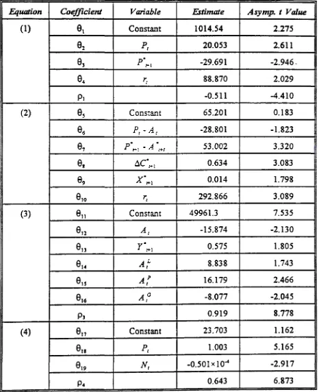
Estimates of the parameters of the model are provided in Table 1, together with their

asymptotic t values. It will be seen that estimates of all 15 structural parameters have the

expected signs and all are significant at the five per cent level (one tail test), thereby

providing strong support for the model specification discussed above. There are, however,

several features of the results for individual equations, which deserve comment. First, the

clear significance of

63

and

a,,

the coefficients of the expected futures price and expected

price spread respectively, appears to provide support for the rational expectations hypothesis

(see also Section V). Moreover, the results for equation (1) support the view that HSS is

essentially a speculative relationship. Similarly, the results for equation (2) suggest that

commitments on the long side of the market are a combination of hedging and speculative

elements, with a strong discretionary component in the hedging activities.

premium in equations (1) and (2) respectively, support an interpretation different from the Kaldor (1953) - Brennan (1958) view of the risk premium. In equation (I) the positive sign

of

6

4 can be explained as follows: an increase in the marginal risk premium cet par will lead

to an increase in the equilibrium futures price, and hence to an increase in the market

commitments of short speculators. In equation (2), an increase in the marginal risk premium cet par will lead to a decrease in the equilibrium price spread, and hence to an increase in the

market commitments of long speculators. These explanations are similar to the '~hedging pressure theory" of Stein (1986, pp. 48-52), although Stein's argument is directed to the effect of a change in the risk premium on price alone.

Thirdly, in equation (3), the consumption relationship, the signs of

6

₁₄ and

6

₁₅ are

consistent with a substitution relationship between Iamb and beef and between pork and beef,

respectively. Moreover, the significance

of6

₁₃,

e

₁₄ and

6

_1, suggests that expected real

income and the prices of lamb and pork are parameters of the demand for beef. Moreover,

the negative sign and significance of el6 suggest that live cattle and feed grain are indeed

complementary inputs.

due, in part, to the thinness of the futures market in the latter part of the sample period.

v

POST-SAMPLE S™ULA TION

A more stringent test of model performance is the ability of the model to forecast key

endogenous variables, against pre-determined criteria, outside the sample period, especially

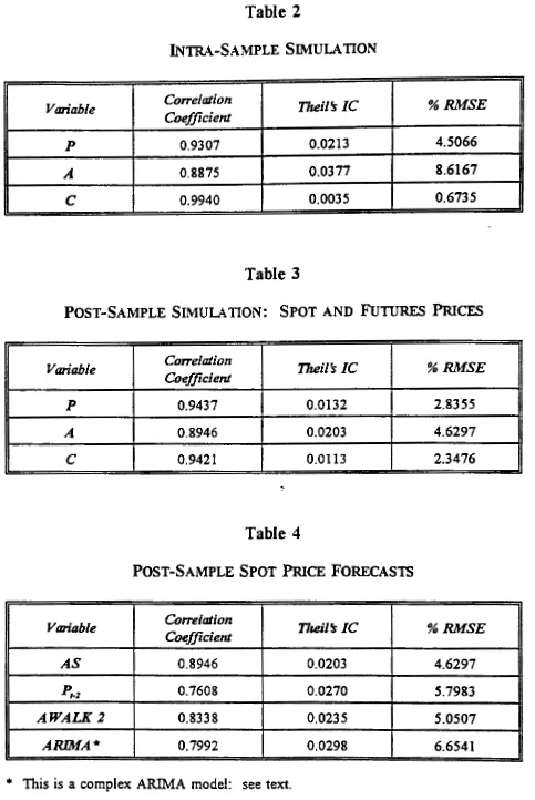
in comparison with alternative forecasts. Table 3 presents an evaluation of (dynamic) two

months ahead forecasts of consumption and the futures and spot prices, for the post-sample

forecast period 1986(03) to 1988(12), comprising 34 monthly observations. Concentrating on

the per cent RMSE criterion, it will be seen first, that the best forecast is again that of

consumption, which has deteriorated compared with the intra-sample forecast, and second that

the better of the two price forecasts is again that of the futures price, and both these price

forecasts have improved significantly compared with intra-sample simulations. This last

outcome with respect to prices provides substantial support for the validity of the model.

The question is then how does the model perform, compared with alternative price

forecasts. Table 4 presents an evaluation of post-sample forecasts of the spot price, two

months ahead, by the model (AS: the same as A in Table 3), compared with three alternative

forecasts. The first alternative forecast is the futures price lagged two months prior to

maturity (

P

₁_

2), the second is a random walk forecast two months ahead,

7

and the third is

a complex ARIMA model of MA terms with lags of one and five months, and an AR term

with a lag of five months. The two latter forecasts are conventional benchmarks in assessing

the forecasting performance of economic models. Table 4 shows that the model developed

in this paper outperforms all the alternative forecasts of the spot price, according to the per

the random walk (AW ALK 2), however, which is the best of the alternative forecasts, is not

statistically significant, at the five per cent level, according to a test of the type proposed in

Granger and Newbold (1986, pp. 278-79).

Turning to a comparison of the spot price forecasts provided by the model (AS) and

by the lagged futures price ( P

1_2), it should be noted that in executing the model-derived

post-sample forecasts, the parameter estimates of the model were updated by one month

following each forecast. Hence, the model and the futures price were placed alwa~s on the

same informational footing during the post-sample period. While the model outperforms the

futures price in making a two-month ahead forecast of the spot price, according to the per

cent RMSE criterion, again this difference is not significant according to the test employed

above. It must be inferred therefore, that the semi-strong efficient markets hypothesis should

not be rejected, because the model evidently does not contain any publicly available

information, which is not reflected in the futures price (see Leuthold and Hartmann, 1979, and

Leuthold and Garcia, 1991 ). This outcome is consistent with the rational expectations

hypothesis employed above, for this assumption implies that agents know the true economic

model driving returns in practice.

VI

CONCLUSIONS

This paper develops and presents estimates of a simultaneous rational expectations model of

the Australian finished (non-storable) live cattle market, using information from both spot and

futures markets. Published studies of simultaneous rational expectations models of such

markets are extremely rare, and only two countries, Australia and the US, have produced data

Australia is the world's leading beef exporting country. The model developed in this

paper contains functional relationships for short hedgers and short speculators combined (there

is no disaggregation of hedging and speculative positions in Australian market commitments

data), long hedgers and long speculators combined, and consumers. The model contains also

a spot price equation, and is completed with a futures market clearing identity.

Augmented Dickey-Fuller and Phillips-Perron tests for unit roots yield ambiguous

results, and the Phillips-Perron tests, taken as definitive, suggest that spot and futures prices,

consumption of beef, expected real income, the price of pork and the price of grain are I(I ),

all other variables being stationary. Johansen co integration tests suggest that the I(l) variables

in each of the structural equations, are cointegrated; in the case of the long hedging-long

speculation relationship, the first difference of the only 1(1) variable, expected consumption

is employed.

Instruments for expectational variables are obtained as fitted values on the set of

pre-determined variables in the model. The structural equations are estimated by instrumental

variables in the absence of serial correlation of the error term, and by non-linear least squares,

if a correction for serial correlation is necessary.

All parameter estimates have the expected signs, and all are statistically significant at

the five per cent level. The signs and significance of the estimated coefficients of the price

and expected price variables in the combined hedger-speculator relationships for the futures

market, provide support for the rational expectations hypothesis. Moreover, the parameter

estimates for the equation referring to short market commitments suggest that this relationship

is essentially speculative; furthermore, there is support for a rival hypothesis of the risk

premium, of the type discussed by Stein ( 1986, pp. 48-52). Parameter estimates suggest also

that market commitments on the long side of the futures market are predominantly those of

processors. Intra-sample the model simulates the futures price with a per cent R.MSE of 4.5%

and the spot price with per cent RMSE of 8.6%, while for consumption of beef the

corresponding figure is 0. 7%. Post-sample, the forecast errors for futures and spot prices

decline to 2.8% and 4.6% respectively, while that for consumption becomes 2.3%. In

post-sample forecasts of the spot price, the model outperforms rival forecasts such as a random

walk(% RMSE 5.1%), an ARIMA model (6.7%) and a lagged futures price (S.8%), although

none of these differences in per cent RMSE between the model and alternative predictors is

-significant. The result in this last comparison, between the model and the lagged futures

pric,e, implies that the semi-strong efficient markets hypothesis cannot be rejected, for there

is no evidence that the model contains information which is not reflected in the futures price.

This outcome, however, is consistent with the employment of the rational expectations

Endnotes

1. Fuller (1976) has shown that the limit distribution of the t statistic for

y

is

independent of the number of lags of 67.. in the equation.

2. For three variables (A, AG, Y) this rejection is made at the 10 per cent level, using the

most appropriate model from the group (7) - ( 10).

3. The instruments employed for the IV estimation of equation (2) are:

HSL,_

₁,

HSL,_

_{2 •}

4. Tests were executed for the presence of ARCH effects (see Engle 1982, 1983) in this

model. An ARCH (p) process postulates that, conditional on information at time (t-1),

an error term e1 is assumed to be normally distributed with mean zero and variance

'!

Although graphs of the partial autocorrelation functions for the squared residuals

revealed various significant lags for the HSS and HSL equations (only), tests of the

hypothesis H(a.P

=

0) suggested that the coefficients were significant at lags p

=

1, 2,

3, 4, 5, 7, 8, 9, 10 for HSS only (see Appendix 5, available on request). It is well

known that high order ARCH effects may be represented by a GARCH (1, 1) process

(see Bollerslev, 1986) where

Accordingly, the HSS equation was re-estimated by maximum likelihood, with the

structural parameters have the expected signs, and are significant at the 5% level (see

Appendix 6, available on request), the estimates of et1 and

'3

1 are not significant.

These last two estimates suppon the view that the GARCH effects in the HSS

equation are not significant, and therefore the results in Table 1 are retained.

5. The instruments for the IV estimation of equation (4) are:

6. Theil's inequality coefficient and per cent RMSE are defined in Pindyck and Rubinfeld

(1981, pp. 362, 364).

7. Random walk forecasts of the spot pnce two months ahead were obtained by

estimating the following model by IvfL: Ar = ~A

1

_

2

where

p

is a parameter to be

estimated. From these estimates fitted vales

At

were obtained, which acted as

Table 1

PARAMETER ESTIMATES

Equation CoefficienJ Variable Ettimate Asymp. t Value

(1)

01

Constant 1014.54 2.275

02

pt 20.053 2.611

03

p•t+I -29.691

-2.946-e4

rr 88.870 2.029

P1

-0.511 -4.410

(2)

es

Constant 65.201 0.183

e6

P1 -At -28.801 -1.823

e,

p·/+I - A .t+I 53.002 3.320

98

~c·t+I 0.634 3.083

e9

x•t+I 0.014 1.798

910

rt 292.866 3.089

(3)

011

Constant 49961.3 7.535

e12

At -15.874 -2.130

e13

y•t+I 0.575 1.805

el4

AL t 8.838 1.743

015

AP

t 16.179 2.466

016

AG t -8.077 -2.045

p3

0.919 8.778

(4)

017

Constant 23.703 1.162

018

P, 1.003 5.165

619

Nt -0.50Ixl04 -2.917

Table 2

INTRA-SAMPLE Sll\1ULA TION

Variable Co"e/ation

Coefficient Theil's IC

%RMSE

p 0.9307 0.0213 4.5066

A 0.8875 0.0377 8.6167

c

0.9940 0.0035 0.6735

Table 3

POST-SAMPLE SIMULATION: SPOT AND FUTURES PRICES

Variable Co"elation

Coefficient Theil's IC %RMSE

p _{0.9437 0.0132} 2.8355

A 0.8946 0.0203 4.6297

c

0.9421 0.0113 2.3476

Table 4

POST-SAMPLE SPOT

PRICE

FORECASTS

Variable Co"e/ation Tlieil's IC %RMSE Coefficient

AS 0.8946 0.0203 4.6297

P,.z

0.7608 0.0270 5.7983

AWALK 2 0.8338 0.0235 5.0507

ARIMA* 0.7992 0.0298 6.6541

REFEREN CFS

ABARE (Australian Bureau of Agricultural and Resource Economics) (1993).

Commodity StaJistical Bulletin, Canberra.

Banerjee, A., J.J. Dolado, J.W. Galbraith & D.F. Hendry (1993). Co-Integration, Error

Correction, and the Econometric Analysis of Non-Stationary Data, Oxfor~ Oxford

University Press.

-Blume, L.E., M.M. Bray & D. Easley (1982). "Introduction to the stability of rational

expectations equilibrium", Journal of Economic Theory, 26: 313-17.

Bollerslev, T. (1986). "Generalized autoregressive conditional heteroskedasticity", Journal

of Econometrics, 31: 307-27.

Bray, M.M. & N.E. Savin (1986). "Rational expectations equilibria, learning and model

specification", Econometrica, 54( 5): 1129-60.

Brennan, M.J. (1958). "The supply of storage", American Economic Review, 48: 50-72.

Cumby, R.E., J. Huizinga & M. Obstfeld (I 983 ). "Two-step two-stage least squares

estimation in models with rational expectations", Journal of Econometrics, 21:

333-55.

Dewbre, J.H. (1981). "Interrelationships between spot and futures markets: some

implications of rational expectations", American Journal of Agricultural

Economics, 63: 926-33.

Dickey, D.A. & W.A. Fuller (1979). "Distribution of the estimators for autoregressive

time series with a unit root", Journal of the American Statistical Association, 74:

327-31.

Dickey, D.A. & W.A. Fuller (1981). "Likelihood ratio statistics for autoregressive time

Engle, R.F. (1982). "Autoregressive conditional heteroskedasticity with estimates of the

variance of U.K. inflation". Econometrica, 50: 987-1008.

Engle, R.F. ( 1983 ). "Estimates of the variance of U.S. inflation based on the ARCH

model", Journal of Money Credit and Banking, 15: 286-301.

Engle, R.F. & C.W.J. Granger (1987). "Co-integration and error correction:

representation, estimation and testing", Econometrica, SS: 251-76.

Evans, G.B.A. & N.E. Savin (1981). "Testing for unit roots: I", Econometrica, 49:

753-79.

Evans, G.B.A. & N.E. Savin (1984). "Testing for unit roots: 2", Econometrica, 52:

1241-68.

Fama, E.F. (1970). "Efficient capital markets: a review of theory and empirical work",

Journal of Finance, 25: 383-417.

Flood, R.P. & P.M. Garber (1980). "A pitfall in estimation of models with rational

expectations", Journal of Monetary Economics, 6: 433-35.

Friedman, D .• G.W. Harrison & J.W. Salmon (1983). "The informational role of futures

markets: some experimental evidence", Chapter 6 in Futures Mancets: Modelling,

Managing and Monitoring Futures Trading, ed. M.E. Streit, Oxford: Basil

Blackwell.

Frydman, R. (1983). "Individual rationality, decentralization and the rational expectations

hypothesis", Chapter 5 in R. Frydman and E.S. Phelps (eds), Individual

Forecasting and Aggregate Outcomes, Cambridge.: Cambridge University Press.

Fuller, W.A. (I 976). Introduction to Statistical Time Series, New York: Wiley.

Giles, D.E.A. & B.A. Goss ( 1981 ). "Futures prices as forecasts of commodity spot prices:

live cattle and wool", Australian Journal of Agricultural Economics, 25(1): 1-13.

soybeans markets with rational expectations", American Joumal of Agricultural

Economics, 67: 749-760.

Goss, B.A. (1972). The Theory of Futures Trading, London: Routledge and Kegan Paul.

Goss, B.A. (1991) (ed.). Rational Expectations and Efficiency in Futures Markets,

London: Routledge.

Goss, B.A., S.G. Avsar & S-C. Chan (1992). "Rational expectations and pnce determination in the U.S. oats market", Economic Record, Special Issue on Futures

Markets, 16-26.

Granger, C.W.J. & P. Newbold (1986). Forecasting Economic Time Series, second ed., London: Academic Press.

Hall, B.H., C. Cummins & R. Schnake (1993). Time Series Processor Version 4.2

Reference Manual, California: Stanford.

Hall, R.E., D.M. Lilien & J. Johnston (1994). "Econometric Views-Micro TSP", User's

Guide, Version 1.0, California, Irvine.

Harrison, G.W. (1992). "Market dynamics, programmed traders and futures markets:

beginning the laboratory search for a smoking gun", Economic Record, Special

Issue on Futures Markets, 46-62.

Johansen, S. (1988). "Statistical analysis of cointegration vectors", Joumal of Economic

Dynamics and Control, 12, 231-54.

Johansen, S. & K. Juselius (1990). "Maximum likelihood estimation and inference on cointegration - with applications to the demand for money", Ox/ ord Bulletin of

Economics and Statistics, 52: 169-210.

Just, R.E. & G. C. Rausser ( 1981 ). "Commodity pnce forecasting with large-scale econometric models and the futures market", American Journal of Agricultural

Kaldor, N. (l 961 ). "Speculation and economic stability", in Essays on Economic Stability

and Growth, London: Duckworth, 17-58.

Kawai, M. (1983). "Spot and futures prices of nonstorable commodities under rational

expectations", Quarterly Joumal of Economics, 97: 235-54.

Keynes, J.M. (1930). A Treatise on Money, Volume 2, London, Macmillan.

Leuthold, R.M. (1972). "Random walks and price trends: the live cattle futures market",

Joumal of Finance, 27: 879-89.

-Leuthold, R.M. (1974). "The price performance on the futures market of a nonstorable

commodity: live beef cattle", American Journal of Agricultural Economics, 56(2):

313-24.

Leuthold, R.M. & P. Garcia (1991). "Assessing market performance: an examination of

livestock futures markets", Chapter 3 in Goss (1991).

Leuthold, R.M. & P.A. Hartmann (1979). "A semi-strong form evaluation of the

efficiency of the hog futures market", American Journal of Agricultural

Economics, 61(3): 482-9.

McCallum, B.T. (1979). "Topics concerning the formulation, estimation and use of

macroeconomic models with rational expectations", Proceedings of the Business

and Economic Statistics Section, pp.65-72, Washington D.C.: American Statistical

Association.

MacKinnon, J.G. (1991). "Critical values for cointegration tests", in R.F. Engle & C.W.J.

Granger (eds), Long-Run Economic Relationships: Readings in Cointegration,

Oxford: Oxford University Press, 267-76.

Maddock, R. & M. Carter (1982). "A child's guide to rational expectations", Journal of

Economic

Literature, 20: 39-51.

Oxford: Basil Blackwell.

Muth, J. ( 1961 ). "Rational expectations and the theory of pnce movements",

Econometrica, 29: 315-35.

Pesaran, M.H. (1987). The Limits to Rational Expectations, Oxford: Basil Blackwell,

(corrected ed. 1989).

Peston, M.H. & B.S. Yamey (1960). "Intertemporal price relationships with forward

. . -:~ .

markets: a method of analysis\ Economica, 27: 355-367.

-Phillips, P.C.B. & P. Perron (1988). "Testing for a unit root in time series regression",

Biometrika, 15, 335-46.

Pindyck, R.S. & D.L. Rubinfeld (1981 ). Econometric Models and Economic Forecasts,

2nd ed., Singapore: McGraw-Hill.

Plott, C.R. & S. Sunder (1982). "Efficiency of experimental security markets with insider information: an application of rational expectations models", Joumal of Political

Economy, 90(4): 663-98.

Said, S.E. & D.A. Dickey (1984). "Testing for unit roots in autoregressive-moving

average models of unknown order", Biometrika, 71(3): 599-607.

Sheffrin, S.M. (1985). Rational Expectations, Cambridge: Cambridge University Press.

Stein, J.L. ( 1961 ). "The simultaneous determination of spot and futures prices", American

Economic Review, 51(5): 1012-25.

Stein, J.L. (1986). The Economics of Futures Markets, Oxford: Basil Blackwell.

Stein, J.L. (1991). International Financial Markets: Integration, Efficiency and

Expectations, Oxford: Blackwell.

Working, H. (1953). "Futures trading and hedging", American Economic Review, 43:

313-343.

Economic Review, June, 52: 431-59.

Wymer, C.R. ( 1977). "Computer programs: TRAN SF manual", Washington DC,

Appendix 1

UNIT ROOT TESTS:

ADF

Calculated

ADF 5% Critical 10% Critical Integration Variable Mode/ Statistic Value Value Order

p _{9 -3.8095 -3.4527 -3.1516 1(0)}

A

9 -3.3090 -3.4527 -3.1516 1(0)_

HSS (=HSL) _{9 -4.7421 -3.4527 -3.1516 I(O)}

c

9 -1.8444 -3.4527 -3.1516 I(l)

(P-A) 7 -3.1357 -2.8889 -2.5812 I(O)

x

8 -3.6586 -2.8892 -2.5813 I(O)

y _{9 -3.3182 -3.4527 -3.1516 I(O)}

r 10 -5.2094 -3.4531 -3.1519 I(O)

AL

₇ -5.1816 -2.8889 -2.5812 1(0)

AP

8 -2.1550 -2.8892 -2.5813 I(l)

N 7 -3.7352 -2.8889 -2.5812 I(O)

Variable p

A

HSS=HSL

c

P-A

x

y r

AL

AP

N

AG

Appendix 2

UNIT ROOT

TESTS:

PHILLIPS-PERRON

Calculated Test Statistic -12.1685 -12.5246 -50.0937 -4.1430 -21.3211

-24.7376

-6.0129

-27.7743

-19.2625

-7.6167

-26.8484

-6.0061

Probability of

Rejection

.3073

.2892

.0095 x

io

-

2

Equation (1) (3) (4) Equation (3)

Appendix 3

JoHANSEN COINTEGRATION PROCEDURE: TRACE TEST

Variables

Ct, At,

~•l'

Af' AtG

Calculated Test Statistic 8.9470 5.4694 9.5650

Appendix 4

Probability of Rejection

.0022

.0174

.0015

No. of Co integrating

Vectors: m

m

~ 1

m ~4

m ~ 1

JoHANSEN COINTEGRA TION PROCEDURE: /..., MAX TEST

Calculated 5% Critical No. of

Variables

Test Statistic Value Cointegrating

Vectors: m

106.3510 77.74 in= 0

A 66.1917 54.64 m ~ 1

Ct, At,

Y,.1,

41.7918 34.55 m ~2

p G

At 'At

21.8950 18.17 m ~3