On the Near-Field Sampling and Truncation Errors in Planar Time-Domain Near-Field to Far-Field Transformation

On the Near-Field Sampling and Truncation Errors in Planar

Time-Domain Near-Field to Far-Field Transformation

Mohammed Serhir*

Abstract—This paper studies the effect of three important parameters in planar time-domain (TD) near-field (NF) to far-field (FF) transformation. These parameters are the NF spatial sampling, NF measurement distance and scan surface truncation. The effect of these parameters over the TD FF accuracy are difficult to predict for Ultra Wide Band antennas. In this paper we aim to choose the optimum NF measurement parameters guaranteeing accurate calculation of the time-domain far-field. This allows the optimization of the computation time and memory requirements. Computations using analytic array of elementary dipoles radiation pattern are used to study the impact of each parameter in time-domain near-field antenna measurement. The comparison of the far-field results are presented in time and frequency domains. In particular, it is shown that the choice of the measurement distance and the size of the scan surface decide predominantly on the frequency band of accurate FF calculation. The used formalism in this paper for the NF to FF transformation is based on the Green’s function.

1. INTRODUCTION

The Ultra Wide Band (UWB) antennas operating over large frequency bandwidth have attracted a lot of interest over wide telecommunication applications [1–5]. The measurement of the radiation pattern of these antennas has to be carried in a wide frequency band, which is time consuming. For these antennas, the time-domain (TD) techniques seem to be more adapted than frequency-domain (FD) techniques. Indeed, using a short pulse, one can measure the antenna transient response covering the frequency band of interest. This measurement is fulfilled using near-field (NF) or far-field (FF) techniques [6].

In TD FF measurements we record the antenna under test (AUT) transient response when it is excited by a specific pulse. The excitation pulse has to cover the frequency band of interest and supply the AUT with enough power that allows the measurement with acceptable signal to noise ratio at far-field distances. In TD NF techniques the tangential components of radiated far-field are collected in the antenna vicinity over a scan surface (planar, cylindrical or spherical). Then, the measured data are transformed to calculate the asymptotic behavior of the antenna far-field. For NF measurement, we use pulse generators providing a trade-off between the output voltage magnitude and a short pulse rise-time for wide frequency band characterization.

For accuracy improvement, the post processing tools such as TD gating technique are used to filter out the multiple reflections occurring during the measurement [7]. The TD techniques allow the radiation pattern measurement in non-anechoic environment as presented in [8]. These are well adapted for the parasitic electromagnetic radiation emitted from electronic devices for electromagnetic compatibility purpose [9]. Also, using TD techniques one can measure the radiation pattern of radar structures fed by non-sinusoidal excitation signals. Particularly, when the feeding system is integrated in the radiating antennas for radar applications.

Received 14 January 2015, Accepted 6 March 2015, Scheduled 14 March 2015

* Corresponding author: Mohammed Serhir ([email protected]).

The main difficulty related to the practical use of NF TD techniques concerns the ability to manage the quantity of measured data. The required computation time and memory storage became problematic for large measurement surface and long-time window (long transient response). The quantity of NF data depends on the used time and spatial sampling criteria. These are determined based on the AUT excitation signal maximum frequency as presented in [10]. Authors in [11–13] present a different NF sampling strategy that aims at representing the NF measurement data using plane polar samples allowing a minimum redundancy in NF sampling. In the FD, Wang in [14] presents a detailed analysis on the theory and practices for planar near-field measurement. The sampling strategies, the NF probe characteristics, the filtering of the NF data and the evanescent modes effect have been addressed. Authors of [15–18] have presented some experimental setups for NF or FF antenna measurement. These papers did not present the sampling strategies used in the NF or FF measurements.

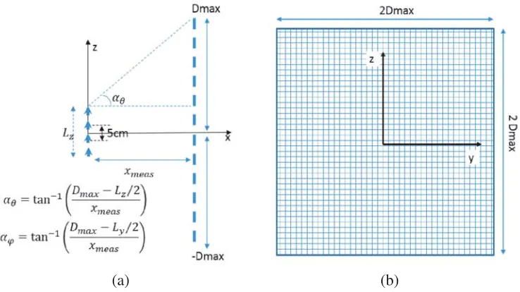
In planar TD near-field antenna measurement, the sampling approach is based on the assumption that the time signal is band-limited to a maximum angular frequency ωmax = 2πc/λmin. This leads to the NF sampling criterion Δy = Δz =λmin/2 and the AUT excitation pulse defines approximately the frequency band of interest (minimum and maximum frequencies). This assumption gives a reduced view of the reality of TD NF measurement practices. Considering the spatial sampling criterion based on the highest frequency of the AUT excitation signal (λmin/2), as presented in [10], does not guarantee the accuracy of the TD far-field calculation. Indeed, the AUTdirectivity depends on the frequency and using the same measurement surface for time-domain FF calculation leads to a frequency dependent truncation error. Also, the NF measurement has to be carried in the radiating NF zone (Fresnel zone). This Fresnel zone distance depends on the AUT dimensions and the operating frequency. For NF TD technique, the measurement distance has to be adapted to avoid the reactive NF zone for low frequencies. These three parameters are responsible of the TD FF errors.

In this paper we propose to determine the AUT TD FF using different sampling criteria and for several NF measurement distances. By comparing the far-field results, we show that the TD FF errors are resulting from NF evanescent modes with low measurement distances, under-sampling and scan surface truncation errors. It is difficult to distinguish between these errors in the TD FF directly. The frequency-domain (FD) comparisons are presented to make out the effect of each error.

In the NF to FF transformation scheme we use the reconstruction formula to rigorously interpolate the NF in the time-domain. We propose a simple and rigorous formulation to calculate the E-field time derivative from the measured E-field as complementary development of the analysis presented in [10]. The computation scheme for NF to FF field transformation is validated using analytic radiating array composed of infinitesimal dipoles. The paper is structured as follows. In Section 2, the NF to FF formalism based on the Green’s function is described and the different formulation needed for our analysis are commented. In Section 3, we present the transformation results and a comparison of the calculated far-field with the actual one in the time and the frequency domains. In Section 4, recommendations and concluding remarks are presented.

2. TIME-DOMAIN NEAR-FIELD TO FAR-FIELD TRANSFORMATION

In this section, we first recall the equations expressing the NF to FF transformation based on the Green’s formulation. The detailed developments can be found in [10]. Then, we present how to calculate rigorously theE-field time derivative using the reconstruction formula. Finally, we present the analytic expressions of infinitesimal dipole radiated field in the TD when it is excited by modulated Gaussian pulse. This infinitesimal dipole is used to generate the TD radiation pattern of our AUT composed of 40 infinitesimal dipoles.

2.1. Time-Domain Near-Field to Far-Field Formalism

the tangential components of the measured NFEmeas.

F(θ, φ, t) =− 1 2πc

+∞

−∞

+∞

−∞ er×

ex×∂ Emeas

∂t (r0, t+er·r0/c)

dy0dz0

with F(θ, φ, t) = lim

r→∞r E(r, t+r/c)

(1)

The measurement surface is defined by−Dmax≤y,z≤Dmax, and (1) is expressed in a truncated form as

F(θ, φ, t) =− 1 2πc

+Dmax

−Dmax

+Dmax

−Dmax

er×

ex×∂ E_∂tmeas (r0, t+er·r0/c)

dy0dz0 (2)

The tangential components of the measured field vector Emeas are collected at a regular grid described by r0 =xmeasex+y ey+z ez with−Dmax≤y,z≤+Dmax. Using the sampling theorem [10], we transform (2) to the following double summation

F(θ, φ, t) =− 1 2πc

Ny

n=−Ny

Nz

m=−Nz

er×

ex×∂ E_∂tmeas(r0mn, t+er·r0mn/c)

Δy0Δz0 (3)

wherer0mn=xmeasex+mΔy ey+nΔz ez,er= cos(φ) sin(θ)ex+ sin(φ) sin(θ)ey+ cos(θ)ez.

We have developed a Matlab routine expressing (3) to calculate the FF using NF data calculated at several measurement distancesx=xmeaswith different sampling criterion Δy, Δz. In (3), the first step

in NF to FF transformation is the calculation of the time derivative of the measured NF at the instant

t+er·r0mn

c . The accuracy of the result depends on the chosen interpolation method. In our analysis,

we will use the reconstruction formula to determine the time derivative of the measured field and to interpolate the field at the required instants.

2.2. The Reconstruction Formula

Let us define a function f(t) where fω is its Fourier transform. f(t) is a band limited function if for

ω≥ωmax

fω =− 1

2π

+∞

−∞ f(t) exp(jωt)dt= 0 (4)

The reconstruction formula allows the exact interpolation of the band limited function f(t) using the discrete points f(t0+lΔt). f(t) is expressed for every t ∈[t0, t0+ (Nt−1)Δt] using the cardinal series as

f(t) =

Nt−1

l=0 sinc

π

t−(t0+lΔt) Δt

f(t0+lΔt) (5)

Using the discrete measurement samples Emeas(t0 +lΔt)1≤l≤N_t−1, one can express accurately

Emeas(t) for everyt∈[t0, t0+ (Nt−1)Δt]. To do this, the Nyquist sampling criterion Δt=π/ωmax has to be respected. The reconstruction formula is used to interpolate the measured E-field as:

Emeas(r0mn, t) =

Nt−1

l=0

h(t)Emeas(r0mn, t0+lΔt) with h(t) = sin

πt−(t0_Δ+_t lΔt)

πt−(t0+lΔt)

Δt

(6)

Fort0 ≤t≤t0+ (Nt−1)Δt, the time derivative of theE-field is expressed rigorously as

∂ Emeas(r0mn, t)

∂t =

Nt−1

l=0

∂h(t)

∂t Emeas(r0mn, t0+lΔt) (7)

where ∂h_∂t(t) = _t−(t1

0+lΔt)(cos(π

t−t0

3 4 5 6 7 8 x 10-9

-1 -0.75 -0.5 -0.25 0 0.25 0.5 0.75 1

0.5 1 1.5 2 2.5 3 3.5 -40

-30 -20 -10 0

(a) (b) (c)

time (s)

s

(

t

) (V)

Excitation Signal Signal Spectrum

Frequency (Hz) _{x 10}9

Magnitude (dB)

Figure 1. (b) The time-domain excitation signal applied to (a) each of the 40 dipoles composing the AUT and (c) the magnitude of the excitation signal spectrum. The maximum of the spectrum is at 2 GHz.

If the sampling Nyquist criterion is respected, (6) and (7) interpolate the E-field and its time derivative. Here, we consider the antenna under test (AUT) composed of infinitesimal dipoles distributed over the planex = 0 as shown in Fig. 1. Each dipole is excited by a pulse and the TD NF is collected over the planex=xmeasat regularly spaced positions. In the next paragraph, we express the analytical

expression of the field radiated by an elemental dipole.

2.3. Transient Radiation of an Infinitesimal Dipole

Let us consider az-polarized elemental dipole placed at the origin of the coordinate system. This dipole is excited bye(t), a sinusoidal current modulated by a Gaussian pulse written as

e(t) =e0sin(βt) exp

−αt2 with α = 2/τ2 (8)

The transient radiated fields Er and Eθ are written in the spherical coordinates system

Er(r, θ, φ, t) = 2η

4πr2 cos(θ)

∂e(t−r/c)

∂t +

c

re(t−r/c)

Eθ(r, θ, φ, t) = _4πrη sin(θ)

∂2e(t−r/c)

c∂t2 +

∂e(t−r/c)

r∂t +

e(t−r/c)

r2

(9)

with

∂e(t)

∂t =e0[βcos(βt)−2αtsin(βt)] exp

−αt2

∂2e(t)

∂t2 =e0

4α2t2−β2−2α sin(βt)−4αβtcos(βt)exp−αt2

(10)

We have used (8)–(10) to generate the tangential componentsEzandEy radiated by 40 elementary

dipoles placed at the plane x = 0. The distance between dipoles is 5 cm, β = 4π109rad/s and

τ = 0.8·10−9s. The dipole distribution is described in Fig. 1. The measurement surface is limited by

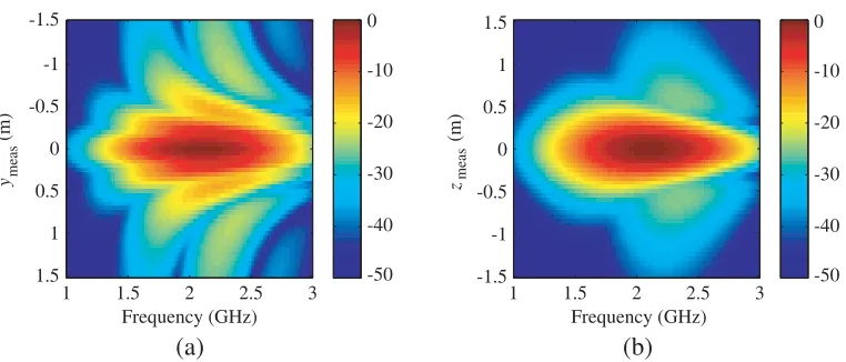
Dmax as shown in Fig. 2 and the TD radiation pattern in the cut planesymeas = 0 and zmeas= 0 are presented in Fig. 3.

3. NUMERICAL RESULTS

In this section we are interested in evaluating the accuracy of the time-domain (TD) FF as a function of the spatial sampling criterion Δyand Δz. The antenna under test (AUT) is composed of 40 elementary dipoles excited by a sinusoidal current modulated by a Gaussian pulse. The NF measured at the distance

(a) (b)

Figure 2. Near-field measurement grid at the distancexmeasfrom the AUT. The tangential components Ey and Ez are regularly recorded over a square surface in thezy plane.

ymeas

(m)

4 6 8 10

-1.5

-1

-0.5

0

0.5

1

1.5 -0.2

-0.1 0 0.1 0.2

zmeas

(m)

4 6 8 10

(a) (b)

time (ns) time (ns)

-1.5

-1

-0.5

0

0.5

1

1.5 -0.2

-0.1 0 0.1 0.2

Figure 3. The Ez (V/m) near-field radiated by the AUT (40 dipoles) as a function of the time. (a) The Ez(V/m) at the plane cutzmeas = 0. (b) TheEz(V/m) at the plane cutymeas= 0.

3.1. The Near-Field Measurement Surface Truncation and the Sampling Criterion

3.1.1. The Time-Domain Far-Field Results Comparison

In the planar rectangular frequency-domain measurement technique, the NF is spatially sampled using the Nyquist rule Δy = Δz = λ/2 with λ being the working wavelength. As presented in [10] the TD NF is spatially sampled based on the AUT excitation signal maximum frequency Δy = Δz = λmin/2 = cπ/ωmax. For a short pulse (UWB antenna), the maximum frequency can beF−3 dB,F−10 dB,F−20 dB,F−30 dB. F−XdB is the frequency for which the magnitude of the excitation pulse spectrum is lower by Xvalue compared with the normalized maximum level (0 dB) of the central frequency. For our case of study, as it is seen in Fig. 1, F−3 dB ≈ 2.3 GHz, F−6 dB ≈ 2.4 GHz,

F−10 dB ≈2.6 GHz,F−20 dB ≈2.8 GHz andF−30 dB≈3 GHz. The maximum magnitude of the excitation signal spectrum corresponds to the central frequency F0 dB = f0 = 2 GHz. We propose to express

Frequency (GHz) 1 1.5 2 2.5 3

-50 -40 -30 -20 -10 0

Frequency (GHz) 1 1.5 2 2.5 3 -1.5

-1 -0.5 0 0.5 1 1.5

ymeas

(m)

-1.5

-1

-0.5

0

0.5

1

1.5

(a) (b)

zmeas

(m)

-50 -40 -30 -20 -10 0

Figure 4. The normalized Ez(dB V/m) NF measured at (xmeas = 50 cm) radiated by the AUT (40

dipoles) as a function of the frequency. (a) The Ez(dB(V/m)) at the plane cut zmeas = 0. (b) The Ez(dB(V/m)) at the plane cut ymeas= 0.

far-field calculated using different χ, we identify the influence of the chosen maximum frequency on the accuracy of the calculated AUT FF. The NF time-axis is sampled using Δt= _3F−1

30 dB to prevent the time-domain aliasing error.

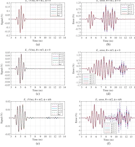
Over the planar surface at the distancexmeas= 50 cm from the AUT, we calculate the near-field at regularly spaced points with Δyχ= Δzχ =λ0/2χand Dmax= 150 cm (10λ0). Then, using (3) and (7), we calculate the FF at the directions (θ=π/2, φ= 0), (θ =π/3, φ= 0), and (θ =π/2, φ=π/6) for

χ= 1.1, 1.2, 1.3, 1.4, 1.5. TheEz component of the FF is presented in Figs. 5(a)–(c)–(e) and compared with the reference FF determined directly from (9) and (10) forr going to infinity. This actual far-field is labeled Ref in Fig. 5. The differences between the calculated FFs and the actual one are quantified using the error expressed in (11). ENFtoFF(θ, φ, t) is the field calculated using NF to FF transformation and ERef(θ, φ, t) is the actual far-field.

Error(θ, φ, t) = 100× ENFtoFF(θ, φ, t)−ERef(θ, φ, t) max (ERef(θ, φ, t))_t0≤t≤t0+(N_t−1)Δt

(11)

The errors of the curves in Fig. 5(a) are presented in Fig. 5(b) for different χ. The errors of the comparisons presented in Fig. 5(c) are plotted in Fig. 5(d). Fig. 5(f) presents the errors of Fig. 5(e). From Figs. 5(b)–(d)–(f) the early-time far-field introduced in [10] as being the part of the radiated FF without the truncation error is visually observed in Fig. 5(e). The measurement surface truncation effect is visible att= 7 ns and 10 ns≤t≤13 ns.

As explained in [10], the effect of the truncation error arrives chronologically after the actual FF signal. This is presented in [10] for a point source. Nevertheless, in Figs. 5(b)–(d)–(f), we notice quantitative differences between the calculated far-fields (FFs) and the actual one even in the time portion of the radiation pattern attributed to early-time far-field (4 ns≤t≤6 ns).

In order to understand the origin of the errors for 4 ns≤t≤6 ns, we have used a larger measurement surface to calculate the FF (Dmax= 300 cm) with the same sampling conditions. The obtained results have shown the same error level for 4 ns ≤ t ≤ 6 ns. These errors are not attributed to the size of the measurement surface. However, we have applied the same analysis (same excitation pulse, same sampling conditions, same measurement distance) for a smaller antenna (4×4) composed of 16 dipoles with 5 cm between dipoles andDmax= 150 cm, the error level is smaller for 4 ns≤t≤6 ns. Moreover, this decreasing tendency is confirmed for 4 dipoles (2×2). The errors for 4 ns ≤ t ≤ 6 ns is directly linked to the size of the AUT.

Signal (V)

-0.15 -0.1 -0.05 0 0.05 0.1 0.15 0.2

χ=1.1 χ=1.2 χ=1.3 χ=1.4 χ=1.5 Ref

Error (%)

-1.25 -1 -0.75 -0.5 -0.25 0 0.25 0.5 0.75 1 1.25

-0.05 -0.04 -0.03 -0.02 -0.01 0 0.01 0.02 0.03 0.04 0.05

Ref

-1.5 -1.25 -1 -0.75 -0.5 -0.25 0 0.25 0.5 0.75 1 1.25 1.5

-0.02 -0.01 0 0.01 0.02

Ref

-8 -6 -4 -2 0 2 4 6 8

(a) (b)

(c) (d)

(e) (f)

Time (ns)

3 4 5 6 7 8 9 10 11 12 13 14

Time (ns)

3 4 5 6 7 8 9 10 11 12 13 14

Time (ns)

3 4 5 6 7 8 9 10 11 12 13 14

Time (ns)

3 4 5 6 7 8 9 10 11 12 13 14

Time (ns)

3 4 5 6 7 8 9 10 11 12 13 14

Time (ns)

3 4 5 6 7 8 9 10 11 12 13 14

-0.2

Signal (V)

Signal (V)

Error (%)

Error (%)

χ=1.1 χ=1.2 χ=1.3 χ=1.4 χ=1.5

χ=1.1 χ=1.2 χ=1.3 χ=1.4 χ=1.5

χ=1.1 χ=1.2 χ=1.3 χ=1.4 χ=1.5

χ=1.1 χ=1.2 χ=1.3 χ=1.4 χ=1.5

χ=1.1 χ=1.2 χ=1.3 χ=1.4 χ=1.5

E z(V/m), θ = π/2, φ = 0

E z (V/m), θ = π/3, φ = 0

E z (V/m), θ = π/2, φ = π/6

E zerror, θ = π/2, φ = 0

E zerror, θ = π/3, φ = 0

E zerror, θ = π/2, φ = π/6

Figure 5. Comparison of the NF to FF transformation results for different sampling criteria Δy= Δz=λ0/2χ, Dmax= 150 cm and xmeas= 50 cm. The TD FF Ez component at (a)θ=π/2 and

φ= 0, (c)θ=π/3 andφ= 0 (e)θ=π/2 andφ=π/6. The errors of Figs. 5(a)–(c)–(e) are respectively (b)θ=π/2 and φ= 0, (d) θ=π/3 andφ= 0 (f)θ=π/2 and φ=π/6.

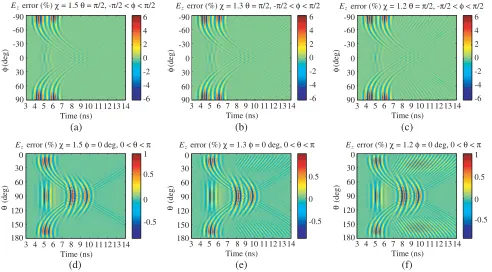
expressed in Fig. 2. This allows an angular FF area free from truncation errors for 30 deg≤θ≤150 deg and −68 deg ≤ φ ≤ 68 deg. This provides an indication and not the exact angular area, especially when the measured field level in the edge of the measurement surface is of comparable levels with the maximum measured field.

φ

(deg)

3 4 5 6 7 8 9 10 11 12 13 14 -90

-60

-30

0

30

60

90 -6

-4 -2 0 2 4 6

θ

(deg)

0

30

60

90

120

150

180

-0.5 0 0.5

(a) (b) (c)

(d) (e) (f)

Time (ns)

3 4 5 6 7 8 9 10 11 12 13 14 Time (ns)

3 4 5 6 7 8 9 10 11 12 13 14 Time (ns)

3 4 5 6 7 8 9 10 11 12 13 14 Time (ns)

3 4 5 6 7 8 9 10 11 12 13 14 Time (ns)

3 4 5 6 7 8 9 10 11 12 13 14 Time (ns)

φ

(deg)

-90

-60

-30

0

30

60

90

φ

(deg)

-90

-60

-30

0

30

60

90

θ

(deg)

0

30

60

90

120

150

180

θ

(deg)

0

30

60

90

120

150

180 -6

-4 -2 0 2 4 6

-6 -4 -2 0 2 4 6

-0.5 0 0.5 1

-0.5 0 0.5 1

E zerror (%) χ = 1.5 θ = π/2, -π/2 < φ < π/2 E z error (%) χ = 1.3 θ = π/2, -π/2 < φ < π/2 E zerror (%) χ = 1.2 θ = π/2, -π/2 < φ < π/2

E z error (%) χ = 1.5 φ = 0 deg, 0 < θ < π E z error (%) χ = 1.3 φ = 0 deg, 0 < θ < π E zerror (%) χ = 1.2 φ = 0 deg, 0 < θ < π

Figure 6. The FFEz component error as a function of time for the plane cutθ=π/2. (a) Forχ= 1.5,

(b) for χ = 1.3, (c) for χ = 1.2. The Ez error as a function of time for the plane cut φ= 0, (d) for

χ= 1.5, (e) forχ= 1.3, (f) for χ= 1.2.

reveal early-time far-field region where the truncation error happens later in time compared with the actual FF. The errors level for 4 ns≤ t≤ 6 ns (actual far-field) is of comparable level with the errors for 7 ns≤t≤10 ns. The errors for 0≤θ≤30 deg, 150 deg≤θ≤180 deg, −90 deg≤φ≤ −68 deg, and 68 deg≤φ≤90 deg are due to the truncation of the measurement surface as predicted byαθ= 70 deg andαφ= 68 deg. In addition, the errors forχ= 1.5 andχ= 1.3 have comparable behavior as it is seen

from Figs. 6(a)–(b)–(d)–(e). Consequently, comparing the TD FF results for this AUT, the weighting factor χ= 1.3 (F−10 dB≈1.3f0) allows a comparable accuracy as χ= 1.5 (F−30 dB≈1.5f0).

3.1.2. The Frequency-Domain Far-Field Results Comparison

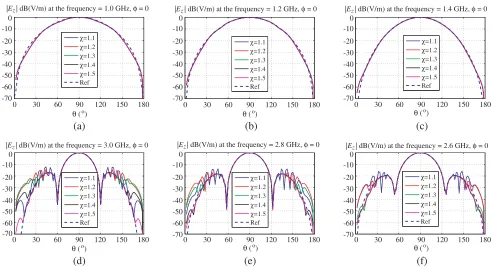
Using the NF sampling criterion Δyχ = Δzχ=λ0/2χ xmeas= 50 cm and Dmax = 150 cm we compare the calculated far-fields in the frequency-domain (FD). These FFs are set by Fourier transforming the previously calculated TD far-fields. The comparisons are carried out at the principal plane cutsθ=π/2 andφ= 0 atF−10 dB(1.4 GHz and 2.6 GHz),F−20 dB(1.2 GHz and 2.8 GHz),F−30 dB(1 GHz and 3 GHz) for different χ.

It is seen in Fig. 4 that the AUT NF truncation level depends on the frequency and the field truncation is more visible in the plane cut zmeas = 0 than the plane cut ymeas = 0. Hence, the

calculated far-field (from NF to FF transformation) is damaged by the truncation error in the cut plane

θ=π/2 more than the cut plane φ= 0. Let us recall that the angular area of the free error FF is for 30 deg≤θ≤150 deg and −68 deg≤φ≤68 deg.

0 30 60 90 120 150 180 χ=1.1

χ=1.2 χ=1.3 χ=1.4 χ=1.5 Ref

χ=1.1 χ=1.2 χ=1.3 χ=1.4 χ=1.5 Ref

χ=1.1 χ=1.2 χ=1.3 χ=1.4 χ=1.5 Ref

χ=1.1 χ=1.2 χ=1.3 χ=1.4 χ=1.5 Ref

χ=1.1 χ=1.2 χ=1.3 χ=1.4 χ=1.5 Ref

χ=1.1 χ=1.2 χ=1.3 χ=1.4 χ=1.5 Ref

(a) (b) (c)

(d) (e) (f)

θ ( )o

0 30 60 90 120 150 180 0 30 60 90 120 150 180

0 30 60 90 120 150 180 0 30 60 90 120 150 180 0 30 60 90 120 150 180

-40 -30 -20 -10 0

-60 -50

-70

-40 -30 -20 -10 0

-60 -50

-70

-40 -30 -20 -10 0

-60 -50

-70

-40 -30 -20 -10 0

-60 -50

-70 -40

-30 -20 -10 0

-60 -50

-70 -40

-30 -20 -10 0

-60 -50

-70

|E z| dB(V/m) at the frequency = 1.0 GHz, φ = 0 |E z| dB(V/m) at the frequency = 1.2 GHz, φ = 0 |E z| dB(V/m) at the frequency = 1.4 GHz, φ = 0

|E z| dB(V/m) at the frequency = 3.0 GHz, φ = 0 |E z| dB(V/m) at the frequency = 2.8 GHz, φ = 0 |E z| dB(V/m) at the frequency = 2.6 GHz, φ = 0

θ ( )o θ ( )o

θ ( )o θ ( )o θ ( )o

Figure 7. Comparison of far-field Ez-component at the plane cut φ = 0 with Dmax = 150 cm,

xmeas = 50 cm and Δy = Δz = λ0/2χ for χ = 1.1, 1.2, 1.3, 1.4, 1.5. (a)–(d) For 1 GHz and 3 GHz (F−30 dB) respectively. (b)–(e) For 1.2 GHz and 2.8 GHz (F−20 dB) respectively. (c)–(f) For 1.4 GHz and 2.6 GHz (F−10 dB) respectively.

The measured NF amplitude at the edge of the measurement surface is only −22.6 dB lower than the maximum NF amplitude in the plane cutzmeas = 0. Consequently, the FF for−68 deg≤φ≤ −40 and 40 deg≤φ≤68 presents important errors.

When the truncation level of the AUT NF measurement data changes significantly as a function of the frequency, the measurement surface has to be adapted to satisfy the same truncation level for every frequency. Otherwise, if the measurement surface stays unchanged, the AUT valuable measurement frequency band is chosen as a function of the truncation level of the measured field. In particular, when measuring the NF of the AUT in the time-domain, we can primarily verify by measuring in the principal cut planesymeas= 0 andzmeas= 0 the level of theE-field truncation level for every measured

frequency by Fourier transforming the time-domain NF. Then, we calculate the NF truncation level by determining the level difference between the maximum E-field and the field level at the measurement surface limit for each frequency. The AUT presents at the cut planezmeas= 0 the truncation levels of

(22.58 dB, 26,18 dB), (33.84 dB, 24.40 dB), (28.78 dB, 33.35 dB) and (27 dB, 26.45 dB) forF−30 dB(1 GHz and 3 GHz), F−20 dB (1.2 GHz and 2.8 GHz), F−10 dB (1.4 GHz and 2.6 GHz) andF−3 dB (1.7 GHz and 2.3 GHz), respectively as presented in Fig. 9.

The AUT NF measurement data guarantee truncation levels less than −30 dB in the plane cut

-90 -60 -30 0 30 60 90 χ=1.1 χ=1.2 χ=1.3 χ=1.4 χ=1.5 Ref χ=1.1 χ=1.2 χ=1.3 χ=1.4 χ=1.5 Ref χ=1.1 χ=1.2 χ=1.3 χ=1.4 χ=1.5 Ref χ=1.1 χ=1.2 χ=1.3 χ=1.4 χ=1.5 Ref χ=1.1 χ=1.2 χ=1.3 χ=1.4 χ=1.5 Ref χ=1.1 χ=1.2 χ=1.3 χ=1.4 χ=1.5 Ref

(a) (b) (c)

(d) (e) (f)

φ ( )o

-40 -30 -20 -10 0 -60 -50 -70

-90 -60 -30 0 30 60 90

φ ( )o

-90 -60 -30 0 30 60 90

φ ( )o

-90 -60 -30 0 30 60 90

φ ( )o

-90 -60 -30 0 30 60 90

φ ( )o

-40 -30 -20 -10 0 -60 -50 -70 -40 -30 -20 -10 0 -60 -50 -70

-90 -60 -30 0 30 60 90

φ ( )o

-40 -30 -20 -10 0 -60 -50 -70 -40 -30 -20 -10 0 -60 -50 -70 -40 -30 -20 -10 0 -60 -50 -70

|E z| dB(V/m) at the frequency = 1.0 GHz, θ = π/2 |E z| dB(V/m) at the frequency = 1.2 GHz, θ = π/2 |E z| dB(V/m) at the frequency = 1.4 GHz, θ = π/2

|E z| dB(V/m) at the frequency = 3.0 GHz, θ = π/2 |E z| dB(V/m) at the frequency = 2.8 GHz, θ = π/2 |E z| dB(V/m) at the frequency = 2.6 GHz, θ = π/2

Figure 8. Comparison of far-field Ez-component at the plane cut θ = π/2 with Dmax = 150 cm,

xmeas = 50 cm and Δy = Δz = λ0/2χ for χ = 1.1, 1.2, 1.3, 1.4, 1.5. (a)–(d) For 1 GHz and 3 GHz (F−30 dB) respectively. (b)–(e) For 1.2 GHz and 2.8 GHz (F−20 dB) respectively. (c)–(f) For 1.4 GHz and 2.6 GHz (F−10 dB) respectively.

-1.5 -1.25 -1-0.75-0.5 -0.25 0 0.25 0.5 0.75 1 1.25 1.5 z_meas (m)

(dB)

F_-30dB 1GHz

F_-30dB 3GHz

F-20dB 1.2GHz

F-20dB 2.8GHz

F_-10dB 1.4GHz

F_-10dB 2.6GHz

F_-3dB 1.7GHz F-3dB 2.3GHz

y_meas (m)

F_-30dB 1GHz

F-30dB 3GHz

F-20dB 1.2GHz

F_-20dB 2.8GHz

F_-10dB 1.4GHz

F_-10dB 2.6GHz

F-3dB 1.7GHz

F-3dB 2.3GHz

-40 -30 -20 -10 0 -50 (a) (b) (dB) -40 -30 -20 -10 0 -50

-1.5 -1.25 -1-0.75-0.5 -0.25 0 0.25 0.5 0.75 1 1.25 1.5

E zdB(V/m) at y meas = 0 E zdB(V/m) at z meas = 0

Figure 9. The normalizedEz NF component forF−30 dB (3 GHz, 1 GHz), F−20 dB (2.8 GHz, 1.2 GHz),

F−10 dB (2.6 GHz, 1.4 GHz), F−3 dB (2.3 GHz, 1.7 GHz). (a) At the plane cut ymeas = 0. (b) At the plane cut zmeas = 0.

3.2. The Near-Field Measurement Distance and the Sampling Criterion

3.2.1. The Time-Domain Far-Field Results Comparison

Let us consider the NF measurement surface with Dmax = 150 cm = 10λ0. We are interested in studying the effect of the NF measurement distances xmeas where the TD NF data are collected with

3 4 5 6 7 8 9 10 11 12 13 14 -5

-4 -3 -2 -1 0 1 2 3 4 5

Time (ns)

Error (%)

x

meas=10cm

x

meas=20cm

x

meas=30cm

x

meas=40cm

x

meas=50cm

3 4 5 6 7 8 9 10 11 12 13 14

Time (ns)

x

meas=10cm

x

meas=20cm

x

meas=30cm

x

meas=40cm

x

meas=50cm

(a) (b)

-4 -3 -2 -1 0 1 2 3 4

Error (%)

E zerror, θ = π/2, φ = 0 E zerror, θ = π/3, φ = 0

Figure 10. The Ez error as a function of time and as a function of the NF measurement distance

(xmeas) for the FF observation points (a) θ=π/2 andφ= 0, (b) θ=π/3 and φ= 0.

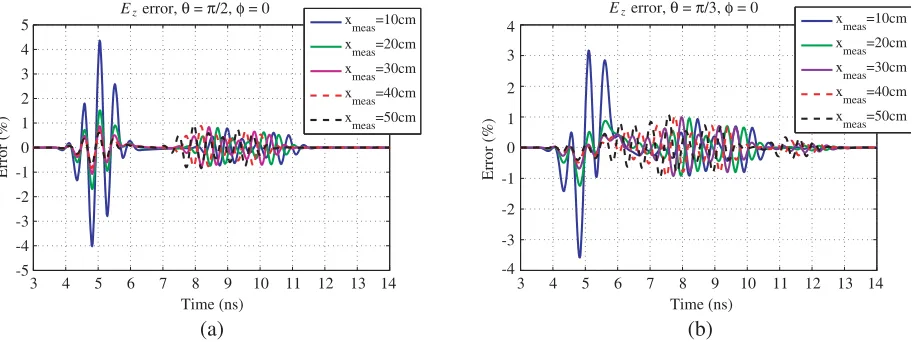
to FF transformation for different measurement distancesxmeas= 10 cm (2λ0/3), 20 cm (4λ0/3), 30 cm (2λ0), 40 cm (8λ0/3) and 50 cm (10λ0/3). The errors resulting from these comparisons are presented in Figs. 10(a) and (b) for the directions (θ=π/2,φ= 0) and (θ=π/3,φ= 0) respectively. As it is seen in Figs. 10(a)–(b), the error depends on the measurement distance, especially for 4 ns≤t≤6 ns. The error values decrease as the measurement distance increases.

Namely, it is difficult to set the limit of the radiating NF zone (Fresnel zone) in the TD NF measurement. The Fresnel zone is defined based on the AUT size and the operating frequency. In TD NF measurement we deal with a frequency band and the NF data measured below the Fresnel zone contain evanescent modes that are probably responsible of the errors for 4 ns ≤t ≤6 ns. Considering smaller antennas, the Fresnel zone is rapidly reached and the errors for 4 ns ≤ t ≤ 6 ns are smaller because less evanescent NF modes are taken into account. In [10] authors have considered a point source and the Fresnel zone is rapidly reached (low evanescent mode) for that case. This explains the early-time far-field free from truncation error as presented in [10].

In addition, from Fig. 10(a), we can isolate the effect of the measurement distance error (4 ns ≤

t≤6 ns) since the truncation error happens later in time and the same error level is observed for every measurement distance for 7 ns ≤ t ≤ 11 ns. If the measurement distance is larger than 2λ0 (30 cm), the error values for xmeas= 2λ0 are equivalent to the error values for xmeas= 50 cm. In contrast with Fig. 10(b), it is difficult to distinguish between the measurement distance error and the truncation error.

3.2.2. The Frequency-Domain Far-Field Results Comparison

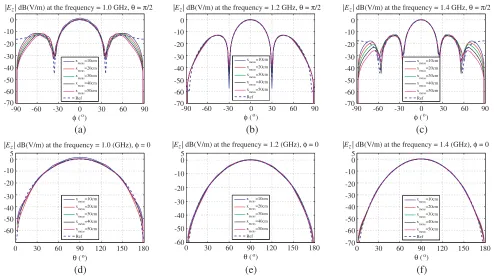
We are interested in studying in frequency-domain the effect of the measurement distance xmeas. The

FF results presented in Fig. 11 are determined by Fourier transforming the time-domain results of the NF to FF transformation of NF data collected atxmeas= 10 cm, 20 cm, 30 cm, 40 cm and 50 cm with the

sampling criterion Δyχ= Δyχ=λ0/3(χ= 1.5). The comparisons presented in Fig. 10 show that TD FF errors decrease as the measurement distance increases. The time-domain errors are helpless to identify which frequency is mostly sensitive to the measurement distance. In contrast, the FD comparisons presented in Figs. 11(a)–(d) show that the frequency (1 GHz) is sensitive to the measurement distance with a maximum difference of 1.47 dB atφ= 0 and 1.45 dB atθ=π/2. The frequency 1.2 GHz presented in Figs. 11(b)–(e) shows a maximum difference of 0.4 dB. The other frequencies (greater than 1.4 GHz) stay unchanged (error≤0.2 dB) since the NF measurement distance is greater than a wavelength.

As a conclusion, usingDmax= 150 cm and xmeas ≥2λ0 the error values are of the same order for

x_meas=10cm x

meas=20cm

x

meas=30cm

x_meas=40cm x_meas=50cm Ref

x

meas=10cm

x

meas=20cm

x_meas=30cm x_meas=40cm x_meas=50cm Ref

x_meas=10cm x meas=20cm x meas=30cm x meas=40cm

x_meas=50cm Ref

x

meas=10cm

x

meas=20cm

x_meas=30cm x_meas=40cm x

meas=50cm

Ref

x_meas=10cm x

meas=20cm

x

meas=30cm

x_meas=40cm x_meas=50cm Ref

x_meas=10cm x_meas=20cm x

meas=30cm

x

meas=40cm

x_meas=50cm Ref

-90 -60 -30 0 30 60 90

(a) (b) (c)

(d) (e) (f)

φ ( )o

-90 -60 -30 0 30 60 90

φ ( )o

-90 -60 -30 0 30 60 90

φ ( )o

0 30 60 90 120 150 180

θ ( )o

0 30 60 90 120 150 180 0 30 60 90 120 150 180

-40 -30 -20 -10 0 -60 -50 -70 -40 -30 -20 -10 0 -60 -50 -70 -40 -30 -20 -10 0 -60 -50 -70 -40 -30 -20 -10 0 -60 -50 5 -40 -30 -20 -10 0 -60 -50 5 -40 -30 -20 -10 0 -60 -50 5 -70

|E _z| dB(V/m) at the frequency = 1.0 GHz, θ = π/2 |E _z| dB(V/m) at the frequency = 1.2 GHz, θ = π/2 |E _z| dB(V/m) at the frequency = 1.4 GHz, θ = π/2

|E z| dB(V/m) at the frequency = 1.0 (GHz), φ = 0 |E z| dB(V/m) at the frequency = 1.2 (GHz), φ = 0 |E z| dB(V/m) at the frequency = 1.4 (GHz), φ = 0

θ ( )o _{θ ( )}o

Figure 11. Comparison of the FF radiation pattern forxmeas= 10 cm, 20 cm, 30 cm, 40 cm and 50 cm at the plane cutθ=π/2, (a) at 1 GHz, (b) at 1.2 GHz, (c) at 1.4 GHz. Comparison of the FF radiation pattern at the plane cutφ= 0, (d) at 1 GHz, (e) at 1.2 GHz, (f) at 1.4 GHz.

in Figs. 5–6–7 it is difficult to predict from TD FF errors the consequences over the AUT radiation pattern in the frequency-domain. For this reason, the frequency-domain (FD) comparisons have been presented to make out the effect of each parameter over the AUT FD FF.

4. CONCLUSION

The effect of three parameters in planar time-domain near-field to far-field transformation have been presented. The followed approach aims to optimize the computation time and memory requirements by studying the near-field sampling measurement criterion. For antennas characterization using the time-domain near-field technique, we have shown that multiple conditions have to be met to correctly calculate the far-field. The size of the measurement surface decides predominantly on the frequency band to consider. The NF spatial truncation is responsible for the frequency limitation. The maximum frequency taken into account depends on the antenna excitation pulse and the behaviour of the AUT near-field directivity as a function of the frequency. Once the maximum frequency is defined, the sampling criterion is based on the Nyquist rate. Specific care has to be applied in choosing the measurement distance which determine the minimum frequency to be considered. Comparisons in TD and FD have been carried out to confirm these assumptions.

REFERENCES

1. Jin, X.-H., X.-D. Huang, C.-H. Cheng, and L. Zhu, “Super-wideband printed asymmetrical dipole antenna,” Progress In Electromagnetics Research Letters, Vol. 27, 117–123, 2011.

3. Akhoondzadeh-Asl, L., M. Fardis, A. Abolghasemi, and G. R. Dadashzadeh, “Frequency and time domain characteristic of a novel notch frequency UWB antenna,” Progress In Electromagnetics Research, Vol. 80, 337–348, 2008.

4. Tuovinen, T., M. Berg, and J. Iinatti, “Analysis of the impedance behaviour for broadband dipoles in proximity of a body tissue: Approach by using antenna equivalent circuits,”Progress In Electromagnetics Research B, Vol. 59, 135–150, 2014.

5. Tsai, C.-L., “A coplanar-strip dipole antenna for broadband circular polarization operation,”

Progress In Electromagnetics Research, Vol. 121, 141–157, 2011.

6. Yaghjian, A. D., “An overview of near-field antenna measurements,” IEEE Transactions on Antennas and Propagation, Vol. 34, No. 1, 30–45, 1986.

7. Blech, M. D., M. M. Leibfritz, R. Hellinger, D. Geier, F. A. Maier, A. M. Pietsch, and T. F. Eibert, “A time domain spherical near-field measurement facility for UWB antennas employing a hardware gating technique,”Adv. Radio Sci., Vol. 8, 243–250, 2010.

8. Jinhwan, K., A. De, T. K. Sarkar, M. Hongsik, W. Zhao, and M. Salazar-Palma, “Free space radiation pattern reconstruction from non-anechoic measurements using an impulse response of the environment,” IEEE Transactions on Antennas and Propagation, Vol. 60, No. 2, 821–831, 2012. 9. Liu, Y. and B. Ravelo, “Fully time-domain scanning of EM near-field radiated by RF circuits,”

Progress In Electromagnetics Research B, Vol. 57, 21–46, 2014.

10. Hansen, T. B. and A. D. Yaghjian,Plane-wave Theory of Time-domain Fields, Near-field Scanning Applications, IEEE Press, New York, 1999.

11. Bucci, O. M., G. D’Elia, and D. Migliore, “Near-field far-field transformation in time domain from optimal plane-polar samples,” IEEE Transactions on Antennas and Propagation, Vol. 46, No. 7, 1084–1088, 1998.

12. Bucci, O. M., G. D’Elia, and D. Migliore, “Optimal time-domain field interpolation from plane-polar samples,”IEEE Transactions on Antennas and Propagation, Vol. 45, No. 6, 989–994, 1997. 13. Bucci, O. M., C. Gennarelli, and C. Savarese, “Representation of electromagnetic fields over

arbitrary surfaces by a finite and nonredundant number of samples,” IEEE Transactions on Antennas and Propagation, Vol. 46, No. 3, 351–359, 1998.

14. Wang, J. J. H., “An examination of the theory and practices of planar near-field measurement,”

IEEE Transactions on Antennas and Propagation, Vol. 36, No. 6, 746–753, 1988.

15. Levitas, B., M. Drozdov, I. Naidionova, S. Jefremov, S. Malyshev, and A. Chizh, “UWB system for time-domain near-field antenna measurement,”2013 European Microwave Conference (EuMC), 388–391, Oct. 6–10, 2013.

16. Serhir, M. and D. Picard, “Development of pulsed antennas measurement facility: Near field antennas measurement in time domain,” 2012 15th International Symposium on Antenna Technology and Applied Electromagnetics (ANTEM), 1–4, Jun. 25–28, 2012.

17. De Jough, R. V., M. Hajian, and L. P. Ligthart, “Antenna time-domain measurement techniques,”

IEEE Antennas and Propagation Magazine, Vol. 39, No. 5, 7–11, 1997.

18. Serhir, M. and D. Picard, “An efficient near field to near or far field transformation in time domain,”