Obtaining and solving systems of equations in
key variables only for the small variants of
AES
Stanislav Bulygin
∗and Michael Brickenstein
†October 9, 2008
Abstract
This work is devoted to attacking the small scale variants of the Advanced Encryption Standard (AES) via systems that contain only the initial key variables. To this end, we introduce a system of equa-tions that naturally arises in the AES, and then eliminate all the inter-mediate variables via normal form reductions. The resulting system in key variables only is solved then. We also consider a possibility to apply our method in the meet-in-the-middle scenario especially with several plaintext/ciphertext pairs. We elaborate on the method fur-ther by looking for subsystems which contain fewer variables and are overdetermined, thus facilitating solving the large system.
Keywords: Algebraic attack, meet-in-the-middle attack, AES, Gr¨obner ba-sis, normal form.
2000 Mathematics Subject Classification: Cryptography 94A60; Poly-nomial ideals, Gr¨obner bases 13P10.
∗Department of Mathematics, University of Kaiserslautern, P.O. Box 3049, 67653
Kaiserslautern, Germany, [email protected]
†Mathematisches Forschungsinstitut Oberwolfach, Schwarzwaldstr. 9-11, 77709
1
Introduction
In this paper we investigate several methods for obtaining and solving key variables only equations, which appear in cryptanalysing the small scale vari-ants of the Advanced Encryption Standard (AES). The cipher Rijndael was chosen as the AES in 2001, and was published as a FIPS 197 standard [30]. AES provides fast and simple symmetric encryptions, while maintaining high resistance to (known) attacks. Simplicity of the AES was criticized since the moment it had appeared, but no one has proposed an attack, which would, at least theoretically, break the AES. We will concentrate on the so-called algebraic attacks. They emerged in the papers of Courtois [21] and Murphy et. al. [29, 18]. The idea is to present the action of the AES block cipher as a system of algebraic equations over a finite field. Then, solving such a system would reveal a secret key. In [21] Courtois and Pieprzyk construct a system over GF(2), whereas in [29] Murphy et. al. propose to consider the system over GF(28). Courtois obtained his system directly from the
AES, wheres Murphy et. al. proposed an embedding of the AES state space to a larger space. Different manipulations and variations of these meth-ods were considered since their appearance. Some works in this area are [17, 16, 12, 13, 32, 29, 18, 19, 1, 2, 21, 15, 31]. So far no method presented any real threat to AES. For better understanding and in order to facilitate experimenting, small scale variants of AES were proposed [19]. We mention also that quite a few multivariate public key cryptosystems and signature schemes were attacked with algebraic methods. Some works in this area in-clude [24, 5, 22, 25].
structures ofPolyBoRi [8], which is the main tool in our experiments, yield an advantage. Also we provide a solid experimental material, which was not done in [32].
The contribution of this paper as we see it is the following two points:
1. Cryptanalytic part. The method of obtaining and solving equations in key variables only coming from the small scale variants of AES. Applying this method in a framework of the meet-in-the-middle-attack, use of several plaintext/ciphertext pairs.
2. Symbolic computations part. Using PolyBoRi as a tool to implement the method in (1). In particular special data structures for operat-ing with Boolean polynomials, computoperat-ing normal forms, and Gr¨obner bases efficiently, supposedly give an advantage against using general purpose computer algebra systems. Therefore the experimental results we present should be considered also from this point.
The paper is organized as follows. In Section 2 we recall necessary notions from computational algebra and give a brief algebraic description of the AES and the small scale variants thereof. In Section 3 we show how corresponding systems of equations over GF(2) are obtained. We note that they actually can be written in different ways. This can result in performance improve-ments, which have partially been presented in [9]. Then we show how to obtain systems with key variables only via normal form computations. Some experiments are discussed. We move further in Section 4 to considering the meet-in-the-middle attack. Some improvements of this attack are then pre-sented in Section 5. We finish with the discussion of obtained results and conclusion.
An extended abstract of a preliminary version of this work is in [7].
2
Background
2.1
Algebraic basics
LetP = GF(2)[x1, . . . , xn] be the polynomial ring over the field GF(2). In
this section we explain notions and state result in terms of GF(2)[x1, . . . , xn],
but most of the things here hold also for a polynomial ring over an arbitrary field. A monomial ordering on P, more precisely, on the set of monomials
{xα =xα1
1 ·. . .·xαnn|α∈ Nn},is a well ordering “>” (i. e. each nonempty set
has a smallest element with respect to “>”) with the following additional property: xα > xβ ⇒ xα+γ > xβ+γ, for γ ∈ Nn. Let f = P
αcα · xα
(cα ∈ GF(2)) be a polynomial. If f 6= 0 then LM(f) denotes the leading
monomial of f, the biggest monomial with respect to “>” occurring in f
with a non-zero coefficient. Denote also by LT(f) the leading termof f, i. e. the leading monomial times the corresponding coefficient. Moreover, we set tail(f) = f−LT(f).
IfF ⊂P is any subset, L (F) denotes theleading idealofF, i. e. the ideal in P generated by {LM(f)|f ∈F\{0}}. A monomial m is called a standard monomial for an ideal I, ifm 6∈L (I).
The S-polynomial of f, g ∈ P\{0} with leading monomials LM(f) = xα
and LM(g) = xβ is defined by
spoly(f, g) = xγ−αf−xγ−βg,
where γ = (max(α1, β1), . . . ,max(αn, βn)). Also, we recall that a finite set
G ⊂ P is called a Gr¨obner basis of an ideal I ⊂ P, if {LM(g)|g ∈ G\{0}}
generates L (I) in the ring P and the inclusion G⊂I holds.
Definition 2.1 (Standard representation, reduced normal form). Let
f, g1, . . . gm ∈P, and let h1, . . . , hm ∈P. Then
f =
m
X
i=1
hi·gi,
is called astandard representation off w. r. t.g1, . . . , gm, ifhi·gi = 0 for alli,
or LM(hi·gi)≤LM(f) otherwise.
Theorem 2.2 (Buchberger’s criterion, cf. e.g Theorem 1.7.3 [26]). Let I be an ideal from GF(2)[x1, . . . , xn] and G = {g1, . . . , gs} ⊂ I. The
following are equivalent:
1. G is a Gr¨obner basis of I.
2. NF(f|G) = 0 for all f ∈I.
3. Each f ∈I has a standard representation with respect to G.
4. G generates I and NF(spoly(gi, gj)|G) = 0 for i, j = 1, . . . , s.
5. Ggenerates I andNF(spoly(gi, gj)|Gij) = 0 for a suitable subsetGij ⊂
G and i, j = 1, . . . , s.
The PolyBoRi framework is designed for Gr¨obner basis computations with the so-calledBoolean polynomials as canonical representatives of residue classes in GF(2)[x1, . . . , xn]/hx21+x1, . . . , x2n+xni. In [10] it is described,
how to apply classical Gr¨obner basis theory for polynomial rings to this quotient ring. On the description and principles of thePolyBoRiframework the reader is referred to [8].
Definition 2.3 (Boolean polynomial). An elementf ∈GF(2)[x1, . . . , xn]
is called a Boolean polynomial, if every variable xi occurs with exponent 0 or
1.
The following two criteria will play a crucial role in explaining our con-struction in Section 3.2.
Proposition 2.4 (Product criterion, cf. e.g. p.63, [26]). Let f, g ∈
GF(2)[x1, . . . , xn] be polynomials such that lcm(LM(f),LM(g)) = LM(f)·
LM(g), then
NF(spoly(f, g)|{f, g}) = 0.
In particular this holds if LM(f) and LM(g) are coprime.
Proposition 2.5 (Linear lead criterion, cf. [8]). Letf ∈GF(2)[x1, . . . , xn]
be a Boolean polynomial such that f =l·g, LM(l) =xi for some iand g any
polynomial, then NF(spoly(f, x2
i +xi)|{f, x21+x1, . . . , x2n+xn}) = 0.
The case g = 1 will be of interest for us.
Definition 2.6 (Elimination orderings). LetR= GF(2)[x1, . . . , xn, y1, . . . ym].
An ordering “>” is called an elimination ordering ofx1, . . . , xn, ifxi > t for
2.2
Description of the AES
For the full description of the AES we refer to [30]. AES in its standard form (the so-called AES-128) operates on rectangular arrays of bytes. So all operations are performed on the 4×4 arrays of bytes. As we have already mentioned, the AES is composed of relatively simple operations in order to ensure its efficient implementation. A set of initial operations that are be-ing executed consecutively composes a round. AES-128 performs 10 rounds, where 9 rounds are the same, and the last 10th round differs a little. We will consider a byte either as an element of GF(28) or as a GF(2)-vector of
length 8 via GF(28) = GF(2)[a]/hm(a)i, where m(a) =a8+a4+a3 +a+ 1
is the Rijndael polynomial. The specifications of such a transformation are given in [30]. The following algebraic description of one round of the AES is from [29].
The AES S-Box. The value of each byte in the array is substituted accord-ing to a table look-up. A result of this table look-up S[·] is the combination of three transformations.
- The input w considered as an element from GF(28) and is mapped to
x=w(−1), where w(−1) is defined by
w(−1) =w254=
w−1 w6= 0,
0 w= 0.
Thus ”AES inversion” is identical to standard field inversion in GF(28) for non-zero field elements with 0(−1) = 0.
- The intermediate value xis regarded as a GF(2)-vector of length 8 and transformed using an (8×8) GF(2)-matrixLA. The transformed vector
LA·x is then regarded in the natural way as an element of GF(28).
- The output of the AES S-Box (substitution box) is (LA·x) + 63 (here
63 is the usual hexadecimal denotation of the byte 11000011), where addition is with respect to GF(2).
The AES linear diffusion (mixing) layer.
- Each row of the array is rotated by a certain number of byte positions.
- Each column of the array is considered to be a GF(28)-vector, and a
In [29] it is shown how to transfer an affine component of an S-Box to the diffusion layer, so that S-Box is represented only by taking the inverse in GF(28). We use this approach in the following discussion.
The AES subkey addition. Each byte of the array is added (with respect to GF(2)) to the corresponding byte from the corresponding array of round keys.
The round key we have just mentioned are created through the so-called
key schedule. Its specification is very similar to the main AES encryption, cf. [30].
2.3
Small scale variants
In [19] C.Cid et. al. proposed the so-called small scaled variants of the AES. The motivation for introducing this notion was that it is very hard to inves-tigate feasibility of algebraic attacks, when one applies them directly to the original AES. So, Cid et. al. proposed to scale down the original cipher AES in terms of:
- the number of rounds n (1≤n≤10);
- the number of rows r in the rectangular representation (r= 1,2,4);
- the number of columns cin the rectangular representation (c= 1,2,4);
- the size e of a word in bits (e= 4,8).
The notation for the scaled-down cipher is SR(n, r, c, e). In this cipher all rounds are the same which is not quite true for the AES: the 10th round differs from the others. But it differs only by an affine mapping, so in principle is the same. Thus we may stick to studying ciphers SR(n, r, c, e). From this prospective, the AES-128 with 10 identical rounds would be the cipher
3
Attacking the AES via composing and
solv-ing a system in key variables only
3.1
Equations over
GF(2)
One can write equations for cryptanalyzing (the small scale variants of) the AES directly bitwise over GF(2). That was an initial proposal of Courtois and Pieprzyk in [21]. There every byte of a 4×4 array is represented by 8 variables (we have 4 variables for the small scale variants with e = 4), each responsible for a corresponding bit in that byte. The equations can then be written in quite a straightforward way. Schematically and abusing notation we can write these equations as
w0 =p+k0, (3.1)
SBOX(xi, wi−1) = 0, i= 1, . . . , n, (3.2)
wi =L(xi) +ki, i= 1, . . . , n, (3.3)
SBOXK(si, ki−1) = 0, i= 1, . . . , n, (3.4)
ki =LK(si) +LK0 (ki−1), i = 1, . . . , n, (3.5)
c=L(xn) +kn. (3.6)
The field equations for all the variables are included. All identifiers are meant to refer to collections of variables (e.g. w0 ={w0,0,0, . . . , w0,0,e−1, . . . , w0,rc−1,0, . . . ,
w0,rc−1,e−1}) except cand p, which are composed of elements in GF(2). Here
SBOX, SBOXK are S-Box transformations for the encryption and the key
schedule resp.; L, LK are affine transformations. Note that operations in
(3.2) and (3.4) are done on each separate byte, whereas in (3.1), (3.3), (3.5), and (3.6) are done on the whole rectangular array. The equations in (3.2) and (3.4) are of degree 2. The equations fromSBOXarise from GF(2e)-equations
xw = 1 translated over GF(2) via x=Pei=0−1xiai and w=Pei=0−1wiai, where
m(a) =a4+a+ 1 = 0 for the casee= 4 andm(a) =a8+a4+a3+a+ 1 = 0
for the case e = 8. So here we suppose that no 0-inversion occurs, which is true with high probability cf. [29]. The equations are listed in the Appendix A.
3.2
Writing the equations differently
cryptanalysis of the AES. Although much effort was put in analyzing the structure of those systems, not much progress is achieved in obtaining com-petitive attacks. In fact, researchers were only able to cryptanalize very ba-sic small scale variants of the AES. For example in [16] and [19] the authors could not go furtherSR(10,1,1,4), SR(2,1,1,8), SR(4,2,1,4), SR(1,2,2,4) for BES equations and SR(10,1,1,4), SR(2,1,1,8) for GF(2)-equations. Al-though it can be shown that one can go a bit further, that does not solve our main goal. The XSL method should also be mentioned here [21]. Initially it was believed that this method might be able to give an attack that could, at least theoretically, break AES, but some evidence afterwards show that probably estimates behind the XSL method were too optimistic ([15]).
Everything said above is a motivation for our present work. We need some preparation. Namely, we will slightly rewrite equations from Section 3.1. In rewriting the equations we aim at the situation where we express every suc-cessive variable via its predecessors. So we rewrite equations (3.1)-(3.6) as follows.
w0 =p+k0, (3.7)
xi =sbox(wi−1), i= 1, . . . , n, (3.8)
wi =L(xi) +ki, i= 1, . . . , n, (3.9)
si =sboxK(ki−1), i= 1, . . . , n, (3.10)
ki =LK(si) +LK0 (ki−1), i= 1, . . . , n, (3.11)
c=L(xn) +kn (3.12)
The field equations on all the variables are added. Here sbox, sboxK are
S-Box transformations for the encryption and the key schedule resp.; L, LK are
affine transformations. How do we achieve the formxi =sbox(wi−1)? Recall
that initially we have degree 2 equations SBOX(xi, wi−1) = 0. Now we
im-pose a block ordering, such thatxi > wi−1 and find a reduced Gr¨obner basis
for these equations. We obtain exactly xi = sbox(wi−1) and one equation
(wi−1,∗,0+ 1). . .(wi−1,∗,e−1+ 1) = 0, which we can drop out by assuming that
the case wi−1,∗,0 = 0, . . . , wi−1,∗,e−1 = 0 does not occur (which is true with
high probability). The same is true for the key schedule. It is interesting to note that actually one can get rid of equations of the type (wi−1,∗,0 +
1). . .(wi−1,∗,e−1 + 1) = 0 without any assumptions on non-occurrence of
0-inversion as above. Recall that an S-Box equation SBOX(x, w) = 0 is written with an assumption that no 0-inversion occurs. Otherwise, one must rewrite GF(2e)-equations x−w2e−2
0-inversions. As we have checked, it turns out that if we write the equa-tions in SBOX this way, we obtain exactly the equations fromsboxwithout
wi−1,∗,0 = 0, . . . , wi−1,∗,e−1 = 0.
Denote now by G the set of polynomials from (3.7)-(3.11) and the com-plete set of field equations for every variable. We denote by the same letter an ideal generated by G. Note thatGcontains both polynomials responsible for encryption/key schedule and the field equations for all the variables. The following holds.
Theorem 3.1. The setGis a Gr¨obner basis of a zero-dimensional ideal with respect to lex ordering induced by k0 < w0 < s1 < x1 < k1 < w1 < · · · <
sn< xn< kn< wn. Variables in each of the variable-blocksk0, w0, . . . , kn, wn
are ordered arbitrarily.
Proof. The claim on dimension follows easily form the fact that the field equations for all the variables are included in G. Now note thatGconsists of the set B of Boolean polynomials with a linear leading term (those coming from encryption/key schedule) and the set F of the field equations. The claim on the Gr¨obner basis follows by applying the product criterion sepa-rately to pairs from the set B and F (Proposition 2.4), and then the linear lead criterion to pairs, where one element is from B and another is from F
(Proposition 2.5).
Remark 3.2. • Other elimination orderings can be used in Theorem 3.1, e.g a block ordering, where each variable-block constitutes one block.
• Clearly the claim thatB is a Gr¨obner basis is trivial due to the product criterion. A distinguishing feature of Theorem above is that we actually work with the field equations included. So a priori it is not clear that
G is a Gr¨obner basis. The result is guaranteed by Proposition 2.5. It is crucial for our method, since field equations are always implicitly included in PolyBoRi.
Note that when e = 4 sbox and sboxK have degree 3 and when e = 8
degree 7. The new equations appear more complex, but the advantage is that we can express each successive variable via its predecessors. See Appendix B for the S-Box equations for both e = 4. For the case e = 8 we have that expressions for x-variables contain resp. 118, 118, 119, 127, 119, 122, 138, 128 monomials.
[4, 17]). It is known that up to now ”a change of the Rijndael polynomial should not affect the strength of the cipher”. It is interesting to see if this is also true in our situation. If we take all 30 irreducible polynomials of degree 8 over GF(2), it can be seen that average number of monomials in the S-Box equations fore= 8 varies from 122 to 139, which is close to 256/2 = 128, half of the number of all Boolean monomials of degree up to 7. So we see that changing Rijndael polynomial to some other irreducible polynomial does not essentially decrease the number of terms in the S-Box equations.
3.3
Gr¨
obner basis shape. Normal forms
Now let us use the Gr¨obner-shape ofGas per Theorem 3.1 to actually obtain equations in initial key variables k0 only. A quite obvious corollary from
Theorem 3.1 shows how to do this.
Corollary 3.3. Denote byR the polynomials (equations) in (3.12). For each
f ∈R,NF(f, G) contains only initial key variables k0.
Note that we can obtain the same result by simply plugging in the vari-ables successively from the beginning to the end and then plugging in in R. Similar approach was proposed for the BES in [32].
For computing a normal form with respect to a system consisting of poly-nomials with pairwise different linear leading terms (and the complete set of field equations), there exist fast, highly specialized algorithms inPolyBoRi. The Buchberger normal form algorithm ([11]) has the disadvantage that it uses iteration over the leading terms of intermediate results and thus its running time gets a quite direct dependency on the number of terms. The special algorithms in PolyBoRi only depend on the ZDD (zero suppressed decision diagram) structure of the involved polynomials [8]. Basically there are two variants:
1. If we have computed the reduced Gr¨obner basis, then all polynomials in it are tail reduced, so the computations are faster. But computing the reduced Gr¨obner basis is quite expensive.
Going back to Corollary 3.3 we see that it is possible to eliminate all variables except the initial key variables.
The following timings that show an application of Corollary 3.3 have been done on a AMD Dual Opteron 2.2 GHz (we have used only one CPU) with 16 GB RAM on Linux using a prerelease version of PolyBoRi 0.5 ([8]). Solving the final system with the key variables is done with the symmgbGF2 algorithm [10] (an advanced version of SlimGB: [6]) implemented in Poly-BoRi. We give the cumulative time for the whole process: normal form reduction and solving.
Cipher time, sec. memory, MB SR(10,2,2,4) 1205 170 SR(10,1,1,4) 0.02 75 SR(10,1,2,4) 0.2 79 SR(10,1,1,8) 2 183
Note that the reduction step takes the lion’s share of the computation, whereas time for the final solving is quite negligible. We could not per-form necessary reductions with F4 implementation in Magma, [23, 14]. We tried NormalForm, Reduce, ReduceGroebnerBasis both with and with-out field equations. The reduction was done with respect to lex ordering.
PolyBoRi- andMagma-examples together with the running scripts can be
downloaded fromhttp://www.mathematik.uni-kl.de/~bulygin/en/files.html. We tried solving systems with Magma and Singular [27] as per
(3.1)-(3.6). We could attack only the full 10 rounds of SR(10,1,1,4) and 3-4 rounds of some 8-bit ciphers. See also results in [19, 16].
We would like to mention an attack based on MRHS linear equations ([31]). In [31] the author was able to break SR(10,1,1,8) in 0.32 sec., which is better than above. Note, however that for key sizes larger than 8, the method of MRHS linear equations needs some bits of a key to be guessed. For instance forSR(10,2,1,8) one needs 8 bits out of 16 to be guessed. Our method does not have such a limitation. It is also notable that for 8 bits known in advance in SR(10,2,1,8) our method needs 4 sec. to execute.
we will have a system ofrceequations inrceunknowns of degreercewith the number of terms approx. 2rce−1 per equation. So solving such a system for
”large” parametersr, c, e is a big challenge. One further point is that Poly-BoRican represent structured polynomials of huge size in a compact way. In this way we can handle carry bits of adders blocks in integrated circuits very efficiently (number of terms 2N −1, memory consumption: 3·N −1·C for
some constant C). For more background about the verification of integrated circuits with computational algebra we refer to [10]. Unfortunately we did not observe such a nice behavior when studying SR-ciphers. In general, we consider block ciphers vulnerable to such a attack, if one of the following conditions, comes true.
1. Some of the equations purely in the key variables are small (in the number of terms and degree).
2. Some of the equations purely in the key variables are structured.
4
Meet-in-the-middle attack
The idea of the meet-in-the-middle attack is not new in cryptanalysis. The ideas of ”meet-in-the-middle” were employed already for attacking DES. The main feature of such attacks is to move from both sides: plaintext and ci-phertext in the ”middle” of a cipher, and there find some binding relations. In algebraic cryptanalysis the technique of ”meet-in-the-middle” is studied in [19, 16] in context of the small scale variants of AES. There the authors propose to divide equations forn rounds into two subsystems: one consisting of equations for rounds 1, . . . , n/2 (here n is assumed to be even), and the one consisting of equations for roundsn/2 + 1, . . . , n. By computing Gr¨obner bases with respect tolexordering the authors get rid of variables that do not appear in rounds n/2 and n/2 + 1. So at the end one deals with a smaller system with the variables from rounds n/2 and n/2 + 1 only. Using also equations from the key schedule it is possible to recover the key. We also mention the use of the meet-in-the-middle principle in [1, 2].
In our approach the meet-in-the-middle attack as described in [19, 16] can be realized in quite a straightforward way. One just has to do ”usual” reductions in rounds 1, . . . , n/2, and then ”reverse” reductions in rounds
n/2 + 1, . . . , n. One then gets equations in k0 and kn from the equations
schedule. In this section our aim will be to illustrate this idea and to see how far can we go in parameters r, c, and e when attacks on two rounds of
SR(2, r, c, e) are considered. Note that here we will essentially use equations obtained from several pairs to make our systems more overdetermined. This is possible, since reduction complexity is not an issue here, see below for the results.
Recall the equations from Section 3.2. Let us write them down again explicitly for the case n = 2 and then discuss how to ”invert” the second round to make the meet-in-the-middle attack possible.
Encryption Key Schedule
w0 =p+k0 (E1) s1 =sboxK(k0) (K1)
x1 =sbox(w0) (E2) k1 =LK(s1) +L0K(k0) (K2)
w1 =L(x1) +k1 (E3) s2 =sboxK(k1) (K3)
x1 =sbox(w0) (E4) k2 =LK(s1) +L0K(k1) (K4)
c=L(x1) +k2 (E5)
The field equations are assumed to be included. Now doing ”usual” reduction in (E1)-(E3) we get equation of the form w1 =”something in k0”, and in
(K1)-(K2) of the form k1 =”someting in k0”. Now we need to ”invert”
equations (E4),(E5),(K3), and (K4) to meet these reduced equations in the middle. The former three equations are easily invertible, namely (E4) inverts as w1 = sbox−1(x2) = sbox(x2), considering that in all SR(n, r, c, e) holds
sbox=sbox−1. Similarly (K3) inverts ask
1 =sbox−K1(s2) =sboxK(s2). Then
(E5) inverts as x2 = L−1(k2 +c), where L−1 is the inverse of the invertible
affine transformation L.
The question remains only with (K4): k2 = LK(s1) +L0K(k1). Let us
represent this linear system in matrix form: (Erce | M | N),
where Erce is a unity matrix rce×rce, and M ∈ M at(GF(2), rce, re), N ∈
M at(GF(2), rce, rce) are full-rank matrices. Obviously, Erce corresponds to
k2-variables, M to s1-, and N to k1-variables. Now if we perform Gaussian
elimination so that matrix M is brought to the diagonal form, we obtain:
T0 | E
re | N0
T00 | 0 | N00
.
HereT0, N0 ∈M at(GF(2), re, rce), T00, N00∈M at(GF(2), rce−re, rce).
0, where A1 is given by matrices T0 and N0, and A2 is given by T00 and N00.
The block s2 = A1(k1, k2) has re equations (the number of components in
s-variables) and the blockA2(k1, k2) = 0 hasrce−reequations. So inverting
equations in this way we get:
Encryption Key Schedule
w0 =p+k0 (E1) s1 =sboxK(k0) (K1)
x1 =sbox(w0) (E2) k1 =LK(s1) +L0K(k0) (K2)
w1 =L(x1) +k1 (E3) k1 =sboxK(s2) (K3’)
w1 =sbox(x2) (E4’) s2 =A1(k1, k2) (K4’)
x2 =L−1(k2+c) (E5’) A2(k1, k2) = 0 (K4”)
Now obviously equations (E3) and (E4’) match through w1-variables which
yields rce equations in k0 and k2 of total degree e−1 from the encryption
part. From the key schedule we getrceequations ink0 andk1 of total degree
e−1 from (K2), re equations in k2 and k1 of total degree e−1 from (K3’)
and rce−relinear equations in k1 and k2 from (K4”). Now note that if we
want to use P plaintext/ciphertext pairs for our attack, then the equations from the key schedule will be the same for all the pairs and the equations from the encryption part will be different. Summarizing we have that using
P pairs we getP rce+rce+re equations of degreee−1 andrce−relinear equations. All these equations are composed of 3rce variables, namely com-ing from k0, k1, and k2.
In order to show how different the meet-in-the-middle representation is from the one we have in Section 3.2, let us compare some important parame-ters of obtained systems, using SR(2,2,2,4) as an example. As is mentioned above, the system in the initial key variables only from Section 3.2 obtained via Corollary 3.3 includes only k0 variables, whereas the one constructed
using the meet-in-the-middle principle includes k0, k1, and k2. The
follow-ing table gives the comparison of some parameters (field equations are not considered):
method # vars # eqs highest deg. av. # of terms ”normal” 1 pair 16 16 9 ≈ 2,500 ”normal” 10 pairs 16 160 9 ≈ 2,500
”m-i-m” 1 pair 48 48 3 10 ”m-i-m” 10 pairs 48 192 3 22
of terms by applying the meet-in-the-middle principle.
We mention here one trick we used in order to reduce size of polynomials in key variables after reductions in the encryption part. Let fi,j denote a
polynomial in key-variables only obtained via equating (E3) and (E4’) for the i-th bit and j-th pair. It turns out that any sum fi,j0+fi,j00 had
approx-imately twice as few terms as any of fi,j (which all have approximately the
same size). So what we do is we replace for every i= 1, . . . , rce each fi,j in
our system by fi,j +fi,j+1 for j = 1, . . . , P −1 and fi,P by fi,P +fi,1. Thus
we obtain an equivalent system where the polynomials responsible for the encryption are reduced in size by a factor of 1.5-4. Note that if fi,j’s were
completely random one would get that any sumfi,j0+fi,j00 has essentially the
same size asfi,j0 orfi,j00. This observation shows that fi,j’s are not quite
ran-dom. But note also that by taking 4-,8-,16-,... sums (i.e. the sums obtained by adding some 4,8,16,.. equations for a given bit positioni) we get the same size as by 2-sums, which one would expect from random polynomials. Also taking 3-sums yields the same size as summands. This phenomenon is to be studied further.
Let us now present some experimental results that were obtained using Poly-BoRi. The timings have been done on a AMD Dual Opteron Processor 242 GB 1.6 GHz (we have used only one CPU) with 8 GB RAM on Linux. The same machine has been used for Magma experiments.
Cipher Key size, bit P tred, sec. ttred, sec. tsolve, sec. mem., MB
SR(2,2,4,4) 32 8 0.1 0.8 1.3 35 SR(2,4,2,4) 32 8 0.2 1.6 1.4 37 SR(2,4,4,4) 64 8 0.3 2.4 3.7 61 SR(2,2,2,8) 32 64 4.0 256 ≈3,300 1,214 SR(2,1,4,8) 32 64 0.4 25.6 ≈950 353 Heretredis time to obtain key-variables-only equations from one pair via
nor-mal form reductions as described above, ttred is the total time for reductions
of all pairs, and tsolve is time to solve the final key-variables-only system.
eight reductions in parallel, and 6 sec. without parallelization. Let us now present some results obtained with Magma 2.14-15.
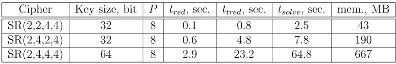
Cipher Key size, bit P tred, sec. ttred, sec. tsolve, sec. mem., MB
SR(2,2,4,4) 32 8 0.1 0.8 2.5 43 SR(2,4,2,4) 32 8 0.6 4.8 7.8 190 SR(2,4,4,4) 64 8 2.9 23.2 64.8 667
We were unable to get any reasonable results forSR(2,2,2,8) andSR(2,1,4,8). Namely it is quite impossible to make reductions as we need. We tried
NormalForm, Reduce, ReduceGroebnerBasis both with and without field equations. Only with
ReduceGroebnerBasis and field equations included could we perform reduc-tions for just one pair’s encryption part in 163 seconds.
Remark 4.1. • In principle it is possible to apply the method for two rounds to the case of three rounds almost with no changes: one just has to do ”forward” reductions in rounds 1-2 and ”reverse” reductions in the third round. We could not break even 32-bit ciphers fore= 4 in any reasonable time with this approach. See the next section on more advanced techniques to tackle the problem.
• The trick on reducing size of polynomials in the encryption part gives a win in efficiency up to 50% for PolyBoRi. Interestingly enough, this tricks considerably slowed down the Magma-computation. So for the table presented above for Magma we did not implement the trick.
• Special data structures employed inPolyBoRi are particularly useful for normal form reductions that we need for obtaining key-variables-only equations. It seems that general purpose computer algebra sys-tems like Magma and Singular are not well suited for the purpose of our approach.
5
Using weak diffusion and guessing some bits
5.1
Overdetermined polynomial systems
in the previous sections to obtain systems in the key variables only, it is pos-sible to get such systems. The relation between variables and equations can be improved by considering more pairs of ciphertext and plaintext. However the number of variables is still quite large.
5.2
Subsets in less variables
The equation systems obtained in Section 4 seem to have more structure than those in Section 3 (at least for a small number of rounds). However most Gr¨obner bases implementations (even if they are optimized for the Boolean case) are quite unaware of this structure. Assuming, that we have have a subsystem, which involves much less variables (which is for certain a result of the weak diffusion layer when working with small number of rounds like 2 or 3), the usual Buchberger’s algorithm would mix them quite strongly with the polynomials that are not included in the considered subsystem, so that their combination would involve more variables. Since more variables usu-ally make computations harder, such an effect is not desirable. So it seems quite appropriate to treat these subsystems in less variables separately to preserve their structure. However, they could describe a complex zero set, whose knowledge might not solve our problem (usually we assume that the complete system has exactly one solution). Actually it is possible in our experiments to overdetermine these subsystems by increasing the number of pairs, so that they will also have only one solution in practice. In this way, solving them will yield the solution for every variable involved in the subsys-tem. Using these values, it will be much easier to solve the complete system by computing a Gr¨obner basis or applying the same trick again. Of course clustering subsystems of polynomials doesn’t seem to be obvious in general. Finding a good (not necessarily the best) solution for identifying such subsystems in polynomial time seems to be related to optimization tech-niques. In our case, we just used a very simple solution: we considered the variable sets of each of the Boolean polynomials that constitute the sys-tem. Let fi, i = 1, . . . , N for some N be polynomials in the key variables
only system. For each i = 1, . . . , N we examine which variables occur in
fi. Denote this set of variables by V ar(fi). Then we collect all the
poly-nomials from the system that contain only variables from V ar(fi) and no
others. Denote the subsystem so obtained by SubSys(fi). Then among all
SubSys(fi), i= 1, . . . , N we look only for overdetermined ones. Among these
oc-curring, i.e. with the smallest |V ar(fi)|. Then for uniqueness of choice we
choose the one subsystem that has among those the most polynomials, i.e. the one with maximal |SubSys(fi)|. This makes the clustering very fast. Of
course, the performance of our computations strongly depends on finding a subsystem in as few variables as possible and also as much overdetermined as possible. While the practical experiments show that the background is quite promising, our method here is quite basic and should be optimized for more complex ciphers to give better results (easier equation systems) to be processed by our solving algorithms.
5.3
Guessing of key bits
Another aspect often applied in cryptanalysis is the guessing of bits in the key. This can be combined quite well with the idea introduced in the pre-vious subsection. Having found a subsystem in less number of variables, we consider small subsets of these variable (preferably some variables out of the initial keyk0). Plugging in trial values for these variables, can yield a system,
which is much easier to solve via Gr¨obner basis computation for each possible value of a trial. This means, that in the presented timings, we really try each combination of these small sets of bits we guess, so no knowledge of them is required for the attack in advance. For example for SR(2,2,2,8) and 64 pairs plugging in just two bits simplified the systems dramatically, such that it was easier to solve four of these systems via the Buchberger’s algorithm, than just one of these systems. While plugging in values provides some speed up, Gr¨obner basis computations can be seen as a good supplement to these search techniques. This is the area, where still much research needs to be done, in a much wider scope: touching both the field of computational al-gebra as well as the very optimized toolset of SAT-solvers. An initial (quite theoretical) publication on these aspects was done in [20].
We don’t have a special selection strategy for the bits at the moment. We tried just taking the first bits of the k0 variables in the subsystem, as well
5.4
Recursion
After having found bits of the key using the techniques in 5.3 and 5.2, we can simplify our key variables only system. This easier system can be analyzed and treated again with the same techniques. In this way, in each step of recursion more bits values will be found. While in this way, a large number of bits might be guessed, the Gr¨obner bases calculation on the subsystems of equations make sure, that we will only continue our search on a specific configuration of guessed bits, if a solution exists.
We next present some results obtained with the method of this section.
Cipher Key size, bit P tred, sec. ttred, sec. tsolve, sec. # b.g.
SR(3,2,4,4) 32 256 0.01 2.56 657 7 SR(2,2,2,8) 32 64 2.7 172.8 356 2 SR(2,2,4,8) 64 256 5.5 1,408 1,131 10
Here ”# b.g.” means the number of bits guessed during the computations.
6
Conclusions and future research
In this paper we presented several methods of obtaining and solving systems of equations coming from algebraic cryptanalysis of small scale variants of AES. The peculiarity of our method in comparison with numerous other at-tempts is that we aim at a situation where only key variables are present in the systems. After showing the method on some small scale variants for 10 rounds we showed how meet-in-the-middle idea can be used in our frame-work. Here also the use of several plaintext/ciphertext pairs facilitated by our method is illustrated. With this approach we could break 2 rounds of e.g.
the small scale variants of AES as well as for other ciphers.
We also would like to mention that application of the described method became possible by using specialized data structures and algorithms imple-mented in PolyBoRi. Examples considered in this paper could be an illus-tration that quite large problems leading to dense systems of equations can still be feasible if optimizations on all levels are made:
• model/problem (combining the equations for several pairs of plaintext/ ciphertext);
• algorithmic (problem specific solving strategies);
• implementation (the PolyBoRi framework).
Acknowledgements
Appendix A: Writing equations as in Section
3.1
Here by (wi) and (xi) we understand the bits coming in and out of an S-Box.
S-Box equations for e= 4:
x2w3+x1w3+x3w2+x2w2+x3w1+x0w0+ 1 = 0,
x3w3+x1w3+x2w2+x3w1+x0w1+x1w0 = 0,
x1w3+x2w2+x0w2+x3w1+x1w1+x2w0 = 0,
x1w3+x0w3+x2w2+x1w2+x3w1+x2w1+x3w0 = 0.
S-Box equations for e= 8:
x7w7+x6w7+x3w7+x2w7+x1w7+x7w6+x4w6 +x3w6+x2w6+x5w5+
+x4w5+x3w5 +x6w4+x5w4+x4w4+x7w3+x6w3+x5w3 +x7w2+x6w2+
+x7w1+x0w0 + 1 = 0,
x6w7+x4w7+x1w7+x7w6+x5w6+x2w6+x6w5 +x3w5+x7w4+x4w4+
+x5w3+x6w2 +x7w1+x0w1+x1w0 = 0,
x7w7+x5w7+x2w7+x6w6+x3w6+x7w5+x4w5 +x5w4+x6w3+x7w2+
+x0w2+x1w1 +x2w0 = 0,
x7w7+x2w7+x1w7+x3w6+x2w6+x4w5+x3w5 +x5w4+x4w4+x6w3+
+x5w3+x0w3 +x7w2+x6w2+x1w2+x7w1+x2w1+x3w0 = 0,
x7w7+x6w7+x1w7+x7w6+x2w6+x3w5+x4w4 +x0w4+x5w3+x1w3+
+x6w2+x2w2 +x7w1+x3w1+x4w0 = 0,
x6w7+x3w7+x1w7+x7w6+x4w6+x2w6+x5w5 +x3w5+x0w5+
+x6w4+x4w4 +x1w4+x7w3+x5w3+x2w3+x6w2+x3w2 +x7w1+
+x4w1+x5w0 = 0,
x7w7+x4w7+x2w7+x5w6+x3w6+x0w6+x6w5 +x4w5+x1w5+x7w4+
+x5w4+x2w4 +x6w3+x3w3+x7w2+x4w2+x5w1+x6w0 = 0,
x7w7+x6w7+x5w7+x2w7+x1w7+x0w7+x7w6 +x6w6+x3w6+x2w6+
+x1w6+x7w5 +x4w5+x3w5+x2w5+x5w4+x4w4+x3w4 +x6w3+x5w3+
Appendix B: Writing equations as in Section
3.2
S-Box equations for e= 4:
x0 =w3w2w1+w2w1w0+w2w1+w2w0+w3+w2+w1 +w0,
x1 =w3w1w0+w3w1+w2w1+w2w0+w1w0+w3,
x2 =w3w2w0+w3w0+w2w0+w1w0+w3+w2,
x3 =w3w2w1+w3w2+w3w1+w3w0+w3+w2+w1.
References
[1] M. Albrecht, C. Cid, ”Algebraic Techniques in Differential Cryptanal-ysis”, available at http://eprint.iacr.org/2008/177.pdf, 2008.
[2] M. Albrecht, C. Cid, ”Algebraic Techniques in Differential Cryptanal-ysis”, Proceedings of the First International Conference on Symbolic Computation and Cryptography, Beijing, China, pp.55–60, 2008.
[3] M. Bardet, J.-C. Faug´ere, and B. Salvy, ”On the complexity of Gr¨obner basis computation of semi-regular overdetermined algebraic equations.” In ICPSS Paris, pp. 71–75, Nov. 2004.
[4] E. Barkan, E. Biham, ”In How Many Ways Can You Write Rijndael?”,
ASIACRYPT 2002, LNCS vol.2501, pp.160–175, 2002.
[5] O. Billet, J. Patain, Y. Seurin, ”Analysis of Intermediate Field Sys-tems”, Proceedings of the First International Conference on Symbolic Computation and Cryptography, Beijing, China, pp.110–117, 2008.
[6] M. Brickenstein, ”Slimgb: Gr¨obner Bases with Slim Polynomials ”,
Zentrum f¨ur Computeralgebra, Kaiserslautern, September, 2005.
[7] M. Brickenstein, S. Bulygin ”Attacking AES via Solving Systems in the Key Variables Only”,Proceedings of the First International Conference on Symbolic Computation and Cryptography, Beijing, China, pp.118– 123, 2008.
[9] M. Brickenstein, A. Dreyer, ”PolyBoRi: A framework for Gr¨obner basis computation with Boolean polynomials”, MEGA’2007, 2007.
[10] M. Brickenstein, A. Dreyer, G. Greuel, M. Wedler, O. Wien-and ”New developments in the theory of Gr¨obner bases and applications to formal verification” Preprint, available at
http://arxiv.org/abs/0801.1177, 2008.
[11] B. Buchberger ”Ein Algorithmus zum Auffinden der Basiselemente des Restklassenrings nach einem nulldimensionalen Polynomideal” Univer-sit¨at Innsbruck, Dissertation, 1965.
[12] J. Buchmann, A. Pyshkin, R.-P. Weinmann, ”A zero-dimensional Groebner basis for AES-128”,FSE 2006, LNCS 4047, pp. 78–88, 2006.
[13] J. Buchmann, A. Pyshkin, R.-P. Weinmann, ”Block Ciphers Sensitive to Groebner Basis Attacks”, CT-RSA 2006, LNCS 3860, pp. 313–331, Springer-Verlag, 2006.
[14] J. J. Cannon, W. Bosma (Eds.) ”Handbook of Magma Functions”, Edition 2.14 (2007).
[15] C. Cid and G. Leurent, ”An Analysis of the XSL Algorithm”, In B.Roy, editor, Advances in Cryptology - ASIACRYPT 2005, vol. 3788 of LNCS, pp.333–352, 2005.
[16] C. Cid, S. Murphy, M.J.B. Robshaw, ”Algebraic Aspects of the Ad-vanced Encryption Standard”, Springer-Verlag, 2006.
[17] C. Cid, S. Murphy and M. Robshaw, ”An Algebraic Framework for Cipher Embeddings”, Proceedings of the 10th IMA International Con-ference on Coding and Cryptography, LNCS 3796, pages 278–289, 2005.
[18] C. Cid, S. Murphy and M. Robshaw, ”Computational and Algebraic Aspects of the Advanced Encryption Standard”,Seventh International Workshop on Computer Algebra in Scientific Computing, CASC 2004, pp. 93–103, St. Petersburg, Russia, 2004.
[20] M. Clegg, J. Edmonds, and R. Impagliazzo, ”Using the Groebner basis algorithm to find proofs of unsatisfiability”, Proceedings of the Twenty-eighth Annual ACM Symposium on the Theory of Computing, pp. 174-183, 1996.
[21] N. Courtois and J. Pieprzyk, ”Cryptanalysis of Block Ciphers with Overdefined Systems of Equations”, in Asiacrypt 2002, LNCS 2501, pp. 267–287, Springer, 2002.
[22] V. Dubois, P.-A. Founque, A.Shamir, J.Stern, ”Practical Cryptanalysis of SFLASH”, Advances in Cryptology - CRYPTO 2007.
[23] J.-C.Faug´ere, ”A new efficient algorithm for computing Gro¨obner bases (F4).” Journal of Pure and Applied Algebra, 139, pp. 61–88, 1999.
[24] J.-C.Faug´ere, A.Joux, ”Algebraic Cryptanalysis of Hidden Field Equa-tion (HFE) Cryptosystem using Gr¨obner Bases”, In Dan Boneh, editor,
Advances in Cryptology - EUROCRYPTO 2003, vol. 2729 of LNCS, pp. 44–60 2003.
[25] J.-C. Faug´ere, L. Perret, ”On the Security of UOV”,Proceedings of the First International Conference on Symbolic Computation and Cryptog-raphy, Beijing, China, pp. 103–109, 2008.
[26] G.-M. Greuel and G. Pfister, ”A SINGULAR Introduction to Commu-tative Algebra”, Springer Verlag, 2008.
[27] G.-M. Greuel, G. Pfister, and H. Sch¨onemann. Singular 3.0. A Computer Algebra System for Polynomial Computations. Cen-tre for Computer Algebra, University of Kaiserslautern (2005).
http://www.singular.uni-kl.de
[28] Martin Albrecht and Gregory Bard, The M4RI Team ”The M4RI Library – Version 20080624”, Website http://m4ri.sagemath.org, 2008.
[30] National Institute of Standards and Technology. Advanced Encryption Standard. FIPS 197. 26 November 2001.
[31] H. Raddum, ”MRHS Equation Systems”, in LNCS 4876, pp. 232–245, 2007.
[32] I. Toli, A. Zanoni, ”An Algebraic Interpretation of AES-128”, in
Advanced Encryption Standard AES: 4th International Conference, AES 2004, Revised Selected and Invited Papers. Hans Dobbertin, Vincent Rijmen, Aleksandra Sowa editors. LNCS 3373, pp. 84–97,