Scholarship@Western
Scholarship@Western
Electronic Thesis and Dissertation Repository
8-29-2019 2:30 PM
New Algorithms for Computing Field of Vision over 2D Grids
New Algorithms for Computing Field of Vision over 2D Grids
Evan Debenham
The University of Western Ontario
Supervisor
Solis-Oba, Roberto
The University of Western Ontario Graduate Program in Computer Science
A thesis submitted in partial fulfillment of the requirements for the degree in Master of Science © Evan Debenham 2019
Follow this and additional works at: https://ir.lib.uwo.ca/etd
Part of the Theory and Algorithms Commons
Recommended Citation Recommended Citation
Debenham, Evan, "New Algorithms for Computing Field of Vision over 2D Grids" (2019). Electronic Thesis and Dissertation Repository. 6552.
https://ir.lib.uwo.ca/etd/6552
This Dissertation/Thesis is brought to you for free and open access by Scholarship@Western. It has been accepted for inclusion in Electronic Thesis and Dissertation Repository by an authorized administrator of
ii
In many computer games checking whether one object is visible from another is very
important. Field of Vision (FOV) refers to the set of locations that are visible from a
specific position in a scene of a computer game. Once computed, an FOV can be used to
quickly determine the visibility of multiple objects from a given position.
This thesis summarizes existing algorithms for FOV computation, describes their
limitations, and presents new algorithms which aim to address these limitations. We first
present an algorithm which makes use of spatial data structures in a way which is new for
FOV calculation. We then present a novel technique which updates a previously
calculated FOV, rather than re-calculating FOV from scratch. We then compare our
algorithms to existing FOV algorithms and show that they provide substantial
improvements to running time and efficiency of memory access.
Keywords
iii
In many computer games checking whether one object is visible from another is very
important. Field of Vision (FOV) refers to the set of locations that are visible from a
specific position in a scene of a computer game. The scene may contain vision-blocking
objects, which prevent some locations within the scene from being visible. Once
computed, an FOV can be used to quickly determine the visibility of multiple objects or
locations from a given position.
This thesis summarizes existing algorithms for FOV computation, describes their
limitations, and presents new algorithms which aim to address these limitations. We first
present an algorithm which uses a more efficient way to store and access vision-blocking
objects within a scene. We then present a novel technique which updates a previously
calculated FOV, rather than re-calculating FOV from scratch. We then compare our
algorithms to existing FOV algorithms and show that they provide substantial
iv
I would like to first express my deepest gratitude to my supervisor, Professor Roberto
Solis-Oba. He has given me constant feedback and guidance throughout the process of
researching and writing this thesis. He did this while offering me the freedom to pursue a
topic outside of his immediate focus of research. I owe a great amount of the final
product of this thesis to his continual commitment and support.
I am also grateful for the help received from other faculty members of the Department of
Computer Science at The University of Western Ontario. In particular I would like to
thank Professor Michael James Katchabaw, whose reading course was a great help
towards the research for this thesis.
I would also like to thank the community of RogueBasin.com for building a collection of
existing open-source work on FOV calculation. Their collection served as the starting
point for this thesis.
Lastly, I would like to thank my parents for their support and advice throughout my
v
Abstract ... ii
Summary for Lay Audience ... iii
Acknowledgements ... iv
Table of Contents ... v
List of Tables ... vii
List of Figures ... viii
Chapter 1 ... 1
1 Background ... 1
1.1 An Introduction to Field of Vision ... 1
1.2 Other Visibility Techniques in Computer Games ... 5
1.3 Existing FOV Algorithms ... 12
1.4 Analysis of Existing FOV Algorithms ... 21
1.5 Correctness Issues with Recursive Shadowcasting ... 28
Chapter 2 ... 30
2 Improving FOV Calculation ... 30
2.1 Grouping Vision-Blocking Cells ... 30
2.2 Splitting Vision-Blocking Groups into Rectangles ... 33
2.3 Storing Rectangles in a Quadtree ... 36
vi
2.6 A Brief Evaluation of Rectangle-Based FOV ... 44
Chapter 3 ... 48
3 Updating an Existing FOV ... 48
3.1 An Overview of FOV Updating ... 48
3.2 Inverting Cones to Update an FOV ... 51
3.3 Ordering Cones for Inversion ... 54
3.4 Checking the Visibility of Cones ... 57
3.5 Rectangle Intersections with a Cone ... 59
3.6 The Cone Inversion Algorithm ... 64
Chapter 4 ... 68
4 Experimental Evaluation of Our FOV Algorithms... 68
4.1 Environments 1 to 4 ... 68
4.2 Environments 5 to 8 ... 77
Chapter 5 ... 87
5 Conclusions and Future Work ... 87
5.1 Conclusions ... 87
5.2 Potential Future Work ... 88
References ... 91
vii
Table 1: Mean running times of our algorithm implementations in environment 1 ... 24
Table 2: Mean running times of Doryen implementations in environment 1 ... 24
Table 3: Mean running times of our algorithm implementations in environment 2 ... 25
Table 4: Mean running times of Doryen implementations in environment 2 ... 25
Table 5: Mean running times of our algorithm implementations in environment 3 ... 26
Table 6: Mean running times of Doryen implementations in environment 3 ... 26
Table 7: Mean running times of Shadowcasting and Rectangle FOV for Figure 22. ... 45
Table 8: Mean running times for Environment 1... 70
Table 9: Mean running times for Environment 2... 70
Table 10: Mean running times for Environment 3... 71
Table 11: Mean running times for Environment 4... 71
Table 12: Mean performance statistics for Environment 1 ... 73
Table 13: Mean performance statistics for Environment 2 ... 74
Table 14: Mean performance statistics for Environment 3 ... 75
Table 15: Mean performance statistics for Environment 4 ... 75
Table 16: Running times for Environment 5. ... 81
Table 17: Running times for Environment 6 ... 82
Table 18: Running times for Environment 7 ... 83
viii
List of Figures
Figure 1: An example of FOV in a game with simple 2D graphics. ... 1
Figure 2: An example of fog of war in League of Legends before image filtering ... 4
Figure 3: A demonstration of shadow mapping. ... 9
Figure 4: A simple grid with a correctly calculated FOV for strict (left), shadowcast (middle), and permissive (right). ... 13
Figure 5: Lines of visibility for shadowcast FOV (left) and strict FOV (right). ... 13
Figure 6: An example of Mass Ray FOV on a simple grid. ... 14
Figure 7: An example of Perimeter Ray FOV on a simple grid. ... 15
Figure 8: An example of Shadowcasting octants, numbered 1-8. ... 16
Figure 9: An example of Recursive Shadowcasting on a simple grid. ... 17
Figure 10: An example of Precise Permissive FOV on a simple grid. ... 19
Figure 11: Examples of each testing environment in a simple 9x9 grid. ... 23
Figure 12: An example of Recursive Shadowcasting producing incorrect output. ... 28
Figure 13: How cells within the region occluded by one vision-blocking cell would be assigned not visible status. ... 31
Figure 14: Cell traversal order of Recursive Shadowcasting for each octant. ... 32
Figure 15: Vision blocking cells (left) being transformed into a rectilinear polygon (center), and then a set of rectangles (right). ... 33
ix
Figure 18: A grid with two vision-blocking cells (left), its quadtree representation with
L=1 (right), and the space represented by each node (middle). ... 36
Figure 19: An example of two adjacent rectangles ... 38
Figure 20: The example from Figure 19, now adjusted to give correct output. ... 39
Figure 21: A figure showing rectangle occlusion and shrinking. ... 41
Figure 22: An example of our testing environment on a 13x13 grid. ... 45
Figure 23: Cones made by a rectangle, S1, and S2. Origins are shown with a dot. ... 49
Figure 24: Rectangle B has cones that are not visible (left), transitioning visible (center), and visible (right). ... 51
Figure 25: A height 2 binary tree of rectangles, approximating a cone. ... 59
Figure 26: Example of a rectangle intersecting both edges of a cone (left), intersecting one edge of a cone (center), and intersecting no edges of a cone (right). ... 62
Figure 27: a primarily horizontal cone with numbered columns ... 63
Figure 28: An example of a rectangle r which may have intersected a binary tree, but not the cone itself ... 64
Figure 29: An example of Environments 1, 2, 3, and 4. ... 69
Figure 30: A simple FOV grid with a single vision-blocking rectangle R. The grid is of size 5x5 on the left and of size 15x15 on the right. ... 78
Figure 31: Environments 5, 6, 7, and 8 on a grid of size 128*128. ... 80
Chapter 1
1
Background
This chapter gives a background on Field of Vision (FOV) and other visibility techniques
in computer games. This includes an explanation of what FOV is, descriptions of several
FOV algorithms, and a brief comparison of them.
1.1
An Introduction to Field of Vision
A field of vision is the set of locations that are visible from a specific position in a scene
of a computer game. FOV is calculated over a two-dimensional finite grid, referred to as
the FOV grid. One grid cell is specified as the source of vision and is referred to as the
FOV sourcecell. Some grid cells are also specified as representing vision-blocking
objects in the game. An FOV algorithm must determine which cells are visible from the
source and which cells are not visible based on the cells that are vision-blocking. The
resulting grid with cells labelled as visible and non-visible is called the field of vision.
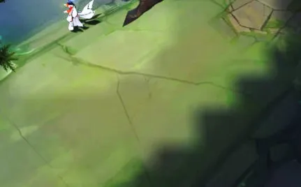
Figure 1 gives an example of FOV in a game. The scene of a simple 2D game is shown
on the left with the FOV grid superimposed in pink. On the right a representation of the
FOV grid is shown: the source cell is marked with an S, vision-blocking cells are marked
with a pattern, and non-visible cells are darkened. FOV grids are usually calculated at a
relatively low resolution, as this provides better performance. In Figure 1 each grid cell
corresponds to a 48x48 pixel region
Calculating an FOV is useful in computer games with a top-down perspective. In these
games the player views the game world from above and thus sees much more of the game
world than an individual character inside the game. This influences game design, and
results in several situations where FOV is useful. For example, these games may wish to
convey to the player which areas of the world their character cannot see by visually
darkening them. This visual effect is referred to as a fog of war and is calculated using
FOV (see Figure 1).
An example of games which use fog of war is the action real-time strategy genre. These
games place two teams of players on a large map with each player controlling one
character. Fog of war is an extremely important visual effect in these games as a player’s
strategy is very dependent on which areas of the game map their character can see. Fog of
war allows a player to quickly see which areas are not visible and make decisions based
on that information. Action real-time strategy games are very popular, the most
significant games in the genre are League of Legends [2] and Defense of The Ancients 2
[3], each with tens of millions of active players.
FOV is also useful for determining visibility, which is a common task for most computer
games. A game environment will likely have objects which obstruct movement and
vision, such as walls or trees, and it is important that game actors interact with these
objects realistically. Actors may need to take visibility into account when making
decisions, such as an enemy checking if it can see the player before attacking them.
The simplest approach to determining visibility is through a line of sight check. For two
points A and B, if the straight line connecting A to B does not intersect any
vision-blocking objects then A can see B. A line of sight check has a non-trivial performance
cost, as there may be many objects within a scene that would need to be checked for
intersection. Despite this, lines of sight can work well in applications where a relatively
Line of sight checks are adequate for calculations involved in actor decision-making, in
games that have a relatively small number of actors who do not need completely accurate
visibility information. As an example, if an enemy turns a corner and wishes to attack the
player, it would not be realistic for them to attack the instant they saw any part of the
player. A game could, for example, perform a single line of sight check from the enemy
to the player once every 250 milliseconds while still maintaining perfectly believable
enemy behavior.
However, games with a top-down perspective may have many actors which need rapid
and accurate visibility information. FOV is useful to these games as it allows visibility
information to be quickly referenced from the FOV grid itself, rather than repeatedly
performing line of sight checks.
Classical real-time strategy games are an example of a genre of game where many
visibility calculations are needed, and line of sight checks are not sufficient. In these
games players control armies of up to hundreds of characters in real-time, and they are
expected to react to player input nearly instantly. Characters may be given an instruction
such as ‘attack the first enemy you see’ and will be expected to immediately attack the
first visible enemy, the moment they become visible, from among hundreds of potential
enemies. Field of vision allows a real-time strategy game to compute the area which a
given character can see once and then check if any enemies are within it, instead of
League of Legends by Riot Games [2] is an excellent example of how FOV grid
resolution affects game quality. The game uses an FOV grid size of 128x128 cells, which
spans the entire game map. This results in a fog of war which is adequate for gameplay
but visually blocky and unrealistic (see Figure 2). The game was originally released in
2009 and has undergone significant development since then, including a visual overhaul
in 2016. As part of that overhaul Riot Games wanted to improve the visual quality of
their fog of war. They experimented with increasing the FOV grid size but deemed it to
be too large of a performance bottleneck [4]. They instead opted to treat the FOV as an
image, and upscale/blur it to increase the perceived quality.
Figure 2 gives an example of FOV in League of Legends before image filtering is
applied. The character at the top-left cannot see the region to the bottom-right because it
is out of its range of visibility. The visible region is circular, but because of the low FOV
resolution the edge of the region appears as a series of jagged lines, rather than a smooth
curve. This is in contrast to the other visual elements of the game, which are well
detailed. This clearly highlights the performance constraints of existing FOV algorithms,
especially as demand for realism in games increases.
1.2
Other Visibility Techniques in Computer Games
There are many other visibility techniques used in computer games which are
conceptually similar to FOV. These problems relate to drawing objects within a game to
the screen. We provide a brief survey of these problems and some of their solutions and
explain why these solutions are not applicable to actor decision-making, where FOV is
useful.
The data which comprises an image displayed on a computer screen is referred to as a
frame buffer. A frame buffer is a two-dimensional array with width and height matching
the resolution of the screen. Each location within this array stores information about one
pixel of an image. Every pixel includes a red, green, and blue component, which combine
to specify the color of that pixel.
Creating a complete frame buffer is a very computationally intensive process, so much so
that specialized hardware is widely available for this sole purpose. This hardware is
referred to as a graphics card, and it contains its own memory and graphics processors
(GPUs) which are designed to rapidly render objects to the frame buffer and then display
that frame buffer on the screen. Graphics cards have led to massive leaps in the number
and complexity of objects which can be rendered on a screen, but their specialized nature
means that they are only suitable for scene rendering within a game. They are not suitable
for processing other aspects of a game, such as actor decision-making, which must be
performed by a computer’s central processor (CPU).
Graphics rendering requires many visibility calculations, and line of sight checks do not
give adequate performance for this task. For instance, if a shadow needs to be drawn, the
computer cannot calculate it with acceptable speed using line of sight, as a line of sight
check would need to be performed for each pixel on the display for every rendered frame.
The most common monitors can display over 2 million pixels at 60 frames per second,
which means that accurately rendering a single shadow would require a ridiculously large
There is a large body of academic work on visibility determination techniques designed
for the graphics card which address various graphical visibility challenges. Examples of
this work include hidden surface removal and shadow calculation. These techniques are
briefly explained below.
If one object is obscured behind another, it is important that the further object is not
rendered to the frame buffer on top of the closer object. Hidden Surface Removal (HSR)
techniques are used to solve this problem, by ensuring that the occluded region of the
further object is not included in the framebuffer for the scene.
The classic approach to correctly rendering objects of varying distances is the painter’s
algorithm [5]. When rendering a scene using the painter’s algorithm, the objects in the
scene are rendered to the frame buffer in order from furthest to closest to the viewpoint.
By rendering objects from furthest to nearest, the painter’s algorithm ensures that closer
objects are always rendered on top of further objects. This approach works well for
simpler scenes but is not useful in modern computer graphics.
Modern GPUs are optimized to render large batches of objects at once, and not one object
at a time. Rendering objects in large batches results in substantially better performance
than rendering individually. Complex scenes are made of many objects, and so batching
them into as few GPU operations as possible is important for performance. This makes
the painter’s algorithm unsuitable for these cases, as it requires that everything be sorted
and then rendered individually.
Modern computer graphics also make use of moving objects and changing terrain. The
painter’s algorithm requires that the objects in a scene be stored in a data structure which
allows for rapid sorting based on the position of the viewpoint, but such data structures
are very slow to build or update. Because of this, the painter’s algorithm is also
unsuitable for scenes with moving objects, as the data structure which stores them would
The more modern approach to correctly and efficiently render objects of varying
distances is to add a per-pixel depth value to the framebuffer, which is called a z-buffer
[6]. When deciding whether to write color values for a given pixel, the GPU compares
the existing z-buffer value for that pixel with the incoming z-buffer value. If the current
z-buffer value is less (i.e. closer) than the incoming value, that pixel is not written to.
Using a z-buffer ensures that distant objects are not rendered over near ones regardless of
the order geometry is rendered in. Z-buffer use is nearly ubiquitous in modern computer
graphics, and it is a standard feature of both GPU hardware and graphics programming
languages [7].
Hidden Surface Removal (HSR) techniques can also improve the performance of
rendering of a 3D scene by identifying which objects in a scene are not visible from the
viewpoint from where the scene is being rendered. As non-visible objects do not affect
the rendered output, skipping the rendering of them improves performance with no
change to the resulting frame buffer. On large complex scenes this provides a substantial
performance improvement over rendering everything regardless of visibility. These HSR
algorithms often make conservative approximations, as it is better to render some small
portion of non-visible objects if it means an HSR algorithm can be much faster. There are
many different HSR algorithms for dealing with different situations in which all or part of
The most simple HSR technique which improves rendering performance is view frustum
culling [8]. The view frustum is the region of space which is visible from the viewpoint
from where the scene is being rendered. Objects which do not intersect the view frustum
can be skipped, as they are guaranteed to not be visible. When testing for intersection
with the view frustum, the shape of objects is often approximated to increase speed, with
the trade-off that objects which are just outside of the frustum will occasionally be
rendered. View frustum culling is universally useful but does not completely remove
non-visible objects on its own. In a scene where closer objects (such as a wall) occlude
further objects, view frustum culling will not be useful for skipping those further objects.
HSR techniques which concern themselves with skipping the rendering of objects which
are occluded behind other objects are called occlusion culling techniques. These
techniques are more complex than techniques like view frustum culling but are very
important for performance in denser environments where a small number of objects may
occlude a large number of objects.
One occlusion culling technique is portal-based occlusion culling [9]. Portal-based
occlusion culling represents a game environment as a number of “rooms” connected via “portals”. Rooms may be any region in 3D space, and Portals are the boundaries between
these regions. This representation can be most intuitively used indoors, where rooms are
actual rooms and portal are doors or windows. These rooms and portals can then be
represented as a graph where rooms are nodes and portals are edges. These rooms are
then pre-processed to generate a ‘potentially visible set’ for a given room R. This
potentially visible set is a collection of all rooms which are visible from at least one point
in R. The set includes at least all nodes adjacent to R in the graph. Then, when rendering
graphics, all rooms which are not in the potentially visible set can be skipped.
Visibility calculations are also useful for rendering shadows in 3D graphics. In computer
graphics, an area is considered to be in shadow if it is not visible from a light source. As
discussed previously, lines of sight are not adequate for this purpose, and so various
Shadow Mapping [10] is the most common technique used for creating shadows cast
from light sources in 3D. To create a shadow map, a z-buffer is rendered from the
perspective of the light source. This z-buffer is then referred to as that light source’s
shadow map. For each pixel of a given surface, its distance from the light source is
compared to the corresponding value on the shadow map, and if the shadow map has a
smaller distance value then that pixel is rendered as being in shadow. A visual example of
this process is shown in Figure 3. This technique is popular due to its performance, but
attaining that performance requires rendering the shadow map at a reduced resolution,
which results in somewhat blocky and imprecise shadows.
Shadow Volumes [11] are an alternative approach to creating shadow effects. A shadow
volume is a representation of the space a shadow occupies, which is created using the
shape of the object casting the shadow. This shadow volume is then used to determine
whether a given surface is in shadow or illuminated. This results in precise (not blocky)
shadows at better performance than high resolution shadow maps, but worse performance
and higher complexity than lower resolution shadow maps.
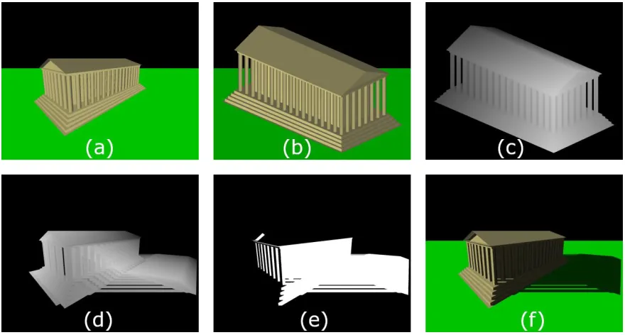
Figure 3: A demonstration of shadow mapping. The images represent:
(a) the scene without shadows, (b) the scene from the perspective of the light source, (c) a visualization of the shadow map (lighter = closer), (d) the shadow map projected onto the scene, (e) a visualization of which pixels are in shadow (white =
Intuitively, it may seem that the above techniques could be suitable for calculating an
FOV. Shadow mapping seems especially suited to this, as it is also a grid-based
representation of visibility from a given source position. However, because these
techniques are designed for GPUs, they are not suitable for processes such as the
computation of actor behavior, which is performed by the CPU.
Algorithms designed for GPUs take advantage of the specialized nature of these
processors and so they would be much slower if they ran on the CPU. Even assuming
these algorithms could produce an FOV, they would not offer competitive performance
when run on the CPU. The output from an FOV algorithm must be available to the CPU,
as it will need to be referenced by other algorithms which run on the CPU, such as those
that control actor behavior.
If algorithms designed for GPUs must be executed on the graphics card, and an FOV
must be available to the CPU, could an FOV be computed on the graphics card, and then
transferred to the CPU? Unfortunately, this will also not offer competitive performance
due to the nature of CPU and graphics card interaction. Graphics cards accept rendering
commands from the CPU, but do not necessarily execute them immediately as they are
received. The CPU does not need to wait while the graphics card does work, so
commands that the CPU issues enter a queue for the graphics card to execute [12]. The
CPU has no access to this queue and cannot know what specific tasks the graphics card is
currently performing. The graphics card may even choose to wait until the queue has
many commands in it before starting execution. Because of this, if the CPU requests an
FOV from the graphics card it has no assurance that the FOV calculation will start in a
timely manner. The CPU may end up waiting until an entire frame buffer is finished
It should be noted that graphics cards can be used for more than just rendering graphics to
a display. Technologies such as Nvidia’s CUDA [13] have enabled graphics cards to run
general-purpose algorithms. These algorithms are faster when run on the graphics card as
they take advantage of its many GPUs. CUDA and similar technologies have enabled
graphics cards to benefit specific areas of Computer Science in a way similar to how they
benefit graphics rendering. Unfortunately, these technologies do nothing to address the
concerns raised previously for FOV calculation using GPUs. This is because there is still
no assurance of when FOV calculations will start, as the graphics card might be busy
with rendering queued graphical operations.
Because of the above limitations, graphical visibility techniques are not able to
effectively calculate an FOV and therefore cannot effectively solve the same problems
which FOV solves. While there is certainly a conceptual overlap between FOV and these
techniques, FOV calculation is a distinct subject with specific applications to processes
1.3
Existing FOV Algorithms
There are several algorithms for calculating FOV. However, these algorithms have not
been formally analyzed to prove their correctness and to compute their complexities.
They are designed by implementors whose primary goals were to produce a game, not
research FOV. To the best of our knowledge this paper is the first effort to perform a
systemic evaluation of these algorithms. Unless otherwise noted, the discussed algorithms
are part of programming folklore, and so have no known author. We summarize the most
popular FOV algorithms and the ones most relevant to our discussion of FOV.
Perhaps the most obvious method for determining the visibility of a cell is to trace a line
from the FOV source to that cell and check for intersection with vision-blocking cells.
Lines cast from the FOV source in a specific direction are a building block of all FOV
algorithms. We refer to these lines as visibility rays, or simply rays.
When describing an FOV algorithm, a rule must be established which dictates the
specific circumstances in which a grid cell is visible from the source cell. By following
such a rule, we can determine whether a calculated FOV is correct. This is important as a
grid discretizes 2D space and implementors may have differing ways that they wish to
define visibility. We refer to these rules as visibility definitions. Consider a source cell S
and destination cell D. We consider the three most common definitions of visibility:
Strict FOV defines that D is visible from S if a ray can be traced from the center of S to
the center of D without intersecting any vision-blocking cells. Many implementors find
this definition overly restrictive, as it results in many non-visible cells.
Shadowcast FOV defines that D is visible from S if a ray can be traced from the center of
S to anywhere on D without intersecting any vision-blocking cells. This definition is
popular as it results in more visible cells than strict FOV and is used by the popular
Recursive Shadowcasting algorithm.
Permissive FOV defines that D is visible from S if a ray can be traced from anywhere on
S to anywhere on D without intersecting any vision-blocking cells. This definition is
It should be noted that the shadowcast and permissive FOV definitions define ‘anywhere
on a cell’ in a way which may not be intuitive. If a ray can reach any point on or in a cell,
including just grazing its edge or corner, then that cell is visible. This behavior comes out
of the desire to have vision-blocking cells be visible, to simulate seeing the face of a wall
or similar vision-blocking object. Strict FOV also accomplishes this by always
considering the destination cell to not be vision-blocking.
Figure 4: A simple grid with a correctly calculated FOV for strict (left), shadowcast (middle), and permissive (right). The rays which define the bounds of visible space
are shown with bolded black lines.
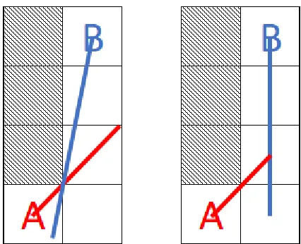
Another important property of an FOV definition is FOV symmetry. An FOV is
symmetrical if visibility, or lack of visibility, is always shared between any two cells (see
Figure 5). This is important for some implementors. Of our three visibility definitions,
strict and permissive are both symmetrical, and shadowcast is not.
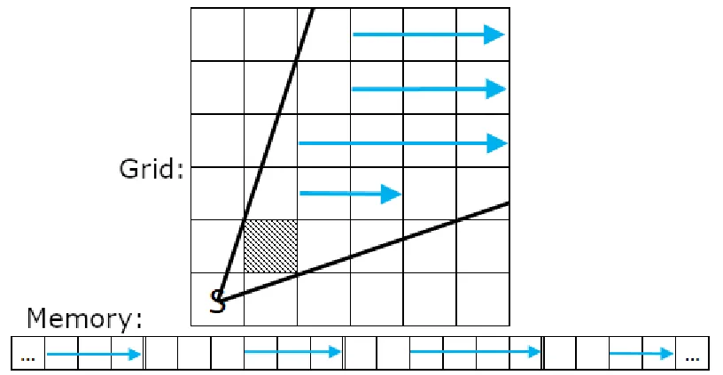
The concept of visibility rays leads to an obvious first FOV algorithm: Mass Ray FOV.
For every cell D within the grid, this algorithm traces a ray from the center of the FOV
source cell to the center of D (see Figure 6). If that ray intersects no vision-blocking cells,
then D is set to visible, otherwise it is set to not visible. Note that a ray is not considered
to intersect with a cell if it just grazes its corner. This produces a correct FOV for the
strict FOV definition.
Figure 6: An example of Mass Ray FOV on a simple grid. Rays cast are on the left, and the calculated FOV grid is on the right. Unobstructed rays are shown in green,
obstructed rays are shown in red.
Mass Ray FOV directly checks for visibility on a per-cell basis. This is in many ways
equivalent to performing a line of sight check for each cell. This leads to very poor
performance, as for an n*n grid, n2 cells must be considered. The number of cells that a
ray intersects increases linearly with n. This gives a total time complexity of O(n3) for
A straightforward optimization to Mass Ray FOV is to assign visibility values to many
cells which intersect a given ray, instead of just the destination cell. An algorithm based
on this approach is Perimeter Ray FOV. Perimeter Ray FOV casts a ray to every cell
along the perimeter of the grid and sets to visible every cell intersected by the ray that is
located between the source and the first vision-blocking cell the ray intersects.
Perimeter Ray FOV has much better performance than mass-ray FOV, as now only 4n-4
rays are cast, instead of n2. This leads to an O(n2) time complexity. However, the
algorithm does check some cells several times. Specifically, cells close to the FOV
source will be set to visible numerous times. This is a large improvement over mass ray
FOV, but shows that there are still ways to improve performance further.
This algorithm produces a result similar to the shadowcast FOV definition, but it is
unfortunately not the same. It is common for there to be some portion of a cell which is
visible from the source, but for the algorithm to not cast a ray in a direction which finds
that visible portion of the cell. This results in Perimeter Ray FOV producing an incorrect
output for the shadowcast FOV definition in many cases (see Figure 7). Increasing the
number of perimeter rays (e.g. one ray cast to each of a cell’s four corners) would reduce
this inaccuracy but would not eliminate it.
Figure 7: An example of Perimeter Ray FOV on a simple grid. Ray casts are on the left, the calculated FOV is in the middle. On the right there is an example of a
As the previous two algorithms have demonstrated, determining visibility by directly
casting a ray to a cell is not ideal. This is not the only way to make use of rays however.
More intelligent FOV algorithms cast rays to the edges of vision-blocking cells, so that
these define the boundary between visible and non-visible space. These algorithms then
traverse through visible cells in increasing order of distance from the FOV source, using
these rays to determine when to stop traversal. This results in few rays being cast and
reduces the number of duplicated cell traversals.
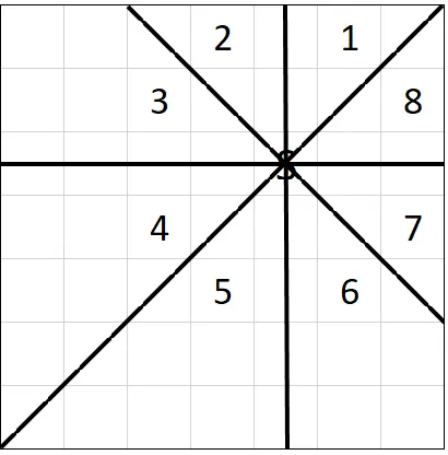
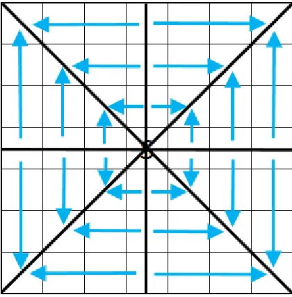
One algorithm based on this approach is Recursive Shadowcasting by Björn Bergström
[14]. This algorithm computes the FOV in 8 iterations, each handling one 45 degree
octant of the FOV grid (see Figure 8). The algorithm described below is written for octant
1, and mirroring operations are performed when accessing cells to process the remaining
7 octants.
Figure 8: An example of Shadowcasting octants, numbered 1-8.
The algorithm for octant 1 processes the cells by rows moving away from the FOV
source. Each row starts at the cell touching the leftmost part of the octant and ends with
the cell touching the rightmost part. When vision blocking cells are encountered, the
algorithm moves the left or right edge of the octant inward for all future rows (see Figure
9). This correctly handles visibility shrinking as vision-blocking cells are encountered. If
the blocking cell is in the middle of a visible region, the algorithm recursively calls itself
to handle the two new visible regions.
Figure 9 shows an example of Recursive Shadowcasting. The algorithm first processes
rows 1 to 3 (shown with blue arrows) without encountering any vision-blocking cells. On
row 4, two vision-blocking cells are encountered, splitting the visible region in two and
causing the algorithm to recursively call itself. The recursive call then processes the
visible region to the left (shown in pink) while the main iteration of the algorithm
continues processing the visible region to the right. Recall that even if a ray just grazes
the edge of a cell, that entire cell must be set to visible.
The algorithm for octant 1 is given below:
Algorithm: recursiveShadowcasting (G, S, T, left, right)
Input: FOV grid G, source cell S, distance integer T, visibility rays left & right
When first called: cells in G are not visible, T is 1, left & right are edges of the octant
Result: cells in G which are visible from S are set to visible
boolean inBlocking = false
for each row R in the part of G between left and right,
starting from T rows away from S {
increment T by 1
for each cell C in R, starting from the cell intersecting left,
and ending with the cell intersecting right {
set C to visible
if C is vision-blocking and inBlocking is false then {
inBlocking = true
recursiveShadowcasting (G, S, T, left,
ray from center of S to top-left corner of C)
} else if C is not vision-blocking and inBlocking is true then {
inBlocking = false
left = ray from center of S to bottom-left corner of C
}
}
if inBlocking is true then return
Another algorithm is Precise Permissive FOV by Jonathon Duerig [15]. This algorithm
produces output for the permissive FOV definition, which makes it an important
alternative to Recursive Shadowcasting for implementors that desire FOV symmetry.
The algorithm has a similar approach to Recursive Shadowcasting. It processes cells
contained within a left and right ray, changes the rays based on encountered
vision-blocking cells, and makes recursive calls when visibility is split. It differs from
Shadowcasting in a few keys ways however:
- Precise Permissive FOV operates on quadrants of the FOV grid, rather than
octants. This means fewer mirroring operations are required.
- Instead of processing the cells by rows, the algorithm uses diagonal lines
(see Figure 10).
- The algorithm performs a recursive call for every blocking cell which is fully
contained between the left and right rays, whereas Shadowcasting performs a
recursive call once for each group of consecutive blocking cells in a row.
- The algorithm casts rays from the edges of the source cell, instead of from the
center, to match the permissive FOV definition.
Figure 10 shows an example of Precise Permissive FOV. First the algorithm moves
though diagonals until it encounters a vision-blocking cell that is fully contained between
the left and right rays. Then, the algorithm recursively calls itself, each iteration now has
its own left and right ray which bound the set of cells that it processes. The final
computed FOV is shown on the right.
The algorithm for quadrant 1 is given below:
Algorithm: precisePermissiveFOV (G, S, T, left, right)
Input: FOV grid G, source cell S, distance integer T, rays left & right
When first called: cells in G are not visible, T is 1, left & right are edges of the quadrant
Result: cells in G which are visible from S are set to visible
for each diagonal line L in the part of G between left and right,
starting from T lines away from S {
increment T by 1
for each cell C in L, starting from the cell intersecting left,
and ending with the cell intersecting right {
Set C to visible
if C is vision-blocking then {
if C is the only cell in L then {
return
} else if C is the first cell in L then {
left = ray from top-left corner of S to bottom-right corner of C
} else if C is the last cell in L then {
right = ray from bottom-right corner of S to top-left corner of C
} else {
precisePermissiveFOV (G, S, T, left,
ray from bottom-right corner of S to top-left corner of C )
left = ray from top-left corner of S to bottom-right corner of C
}
}
}
1.4
Analysis of Existing FOV Algorithms
We now analyze the performance of the four FOV algorithms discussed in Chapter 1.3.
This analysis will help highlight the performance characteristics of these algorithms, so
that we may then propose improvements. The existing research on FOV algorithms is
very limited. To the best of our knowledge, there is a single study of FOV algorithms
made by Jice in 2009 [16]. This study tests several FOV algorithms in a variety of cases
but has several shortcomings which we address below.
Firstly, Jice ran each FOV algorithm multiple times with the same input and reported
statistics on the performance results. Repeatedly running an FOV algorithm may be
problematic because the performance of each run of the algorithm will be affected by the
CPU cache. The CPU cache is a relatively small amount of extremely fast memory which
the computer attempts to populate with recently referenced data. The FOV algorithms
which we have described in Chapter 1.3 perform large numbers of memory accesses, and
so having some or all of the FOV grid stored in the cache will substantially enhance their
performance. However, in a computer game the FOV will be computed as needed, in
between many other computations, and so the FOV grid would not be consistently stored
in the cache. Running FOV algorithms many times without ensuring the grid is not
present in the cache will result in unrealistic performance data. In our analysis each run of
an FOV algorithm uses an entirely new grid. This ensures that the CPU cache will be
filled with old FOV grids which the algorithms are no longer using, thus effectively
clearing it.
The work in [16] also compares the differences in the visibility grid computed by the
tested FOV algorithms. Such an analysis may be helpful to implementors who wish to
decide on a visibility definition, but it is not useful for comparing the performance of
FOV algorithms. Jice assigns a score to each algorithm based on its visual output, but
even Jice admits that the scoring system is largely arbitrary. This is why in our analysis
we use a limited number of visibility definitions and do not attempt to rank them, so as to
The work in [16] uses FOV algorithm implementations present in the Doryen library [12]
(also referred to as LIBTCOD). This library provides many game related functions, but it
is not specifically focused on providing a lightweight or efficient implementation of FOV
algorithms. In [16] no comparisons are made between the implementations in the Doryen
library and other implementations of FOV algorithms. Because of this, the results
presented in [16] may be influenced by inefficiencies present in the Doryen library. We
compare the Doryen library’s implementation of FOV algorithms to our own
implementations to determine if such inefficiencies exist.
Finally, while [16] presents overall performance statistics for each FOV algorithm
studied, it does not examine what causes differences in performance between the
algorithms. Some algorithms are shown to have superior performance in certain
situations, but [16] makes no attempt to determine why. We will choose test cases which
highlight specific performance characteristics in order to better understand differences
between each FOV algorithm.
We tested all four algorithms described in Chapter 1.3. We used our own
implementations of each algorithm as well as the Doryen implementation of Perimeter
Ray FOV, Recursive Shadowcasting, and Permissive FOV. The Doryen library does not
include an implementation of Mass Ray FOV. For all algorithms we did not consider the
Figure 11: Examples of each testing environment in a simple 9x9 grid
We tested using three environments, shown in Figure 11. Each environment was tested at
grid sizes ranging from 128*128 to 4096*4096. These sizes cover a realistic range of
values which game implementors may choose to use. Square grids were chosen as they
are the most common environment shape used by games which use FOV. This range
includes the current grid size of League of Legends [2] (128*128) and the size that
League of Legends visually upscales its grid to (512*512) [4].
Note that while monitors commonly have a display resolution below 4096*4096, game
environments may be much larger in size than the area visible on screen. This means that
if the FOV grid has a size greater than the monitor’s resolution, only a region of the grid
will be visible.
The first environment is an entirely empty FOV grid, which is the worst-case with respect
to the number of cells which must be set to visible. This environment is purely a test of
how efficiently each algorithm assigns visibility statuses to cells.
The second environment is a 5x5 enclosed space with the FOV source in its center. This
is almost a best-case scenario with respect to the number of cells which must be set to
visible. This effectively tests how each algorithm performs when the number of cells
which are visible is very small, regardless of the size of the FOV grid.
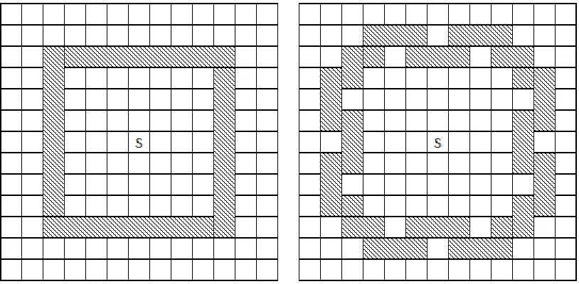
The third environment is a mostly enclosed FOV grid with a three cell wide corridor
extending in each cardinal direction. This environment is designed to be close to a
worst-case scenario for Recursive Shadowcasting and Permissive FOV when compared to other
Table 1: Mean running times of our algorithm implementations in environment 1
Grid Size Mass Ray Perimeter Ray Shadowcasting Permissive
128*128 5,160 μs 257 μs 75 μs 95 μs
256*256 37,965 μs 1,004 μs 343 μs 317 μs
512*512 291,654 μs 4,161 μs 1,744 μs 2,022 μs
1024*1024 2,319,475 μs 21,444 μs 11,720 μs 9,341 μs
2048*2048 19,257,575 μs 112,544 μs 49,381 μs 47,443 μs
4096*4096 178,968,245 μs 636,215 μs 242,105 μs 394,429 μs
Table 2: Mean running times of Doryen implementations in environment 1
Grid Size Perimeter Ray Shadowcasting Permissive
128*128 785 μs 299 μs 728 μs
256*256 3448 μs 1,204 μs 2,911 μs
512*512 13,993 μs 4,566 μs 11,913 μs
1024*1024 65,036 μs 19,592 μs 50,597 μs
2048*2048 264,784 μs 80,121 μs 180,286 μs
4096*4096 1,065,233 μs 339,157 μs 710,267 μs
The O(n3) time complexity of Mass Ray FOV is clearly shown in Table 1: the algorithm
is substantially slower than all others and its running time increases by roughly a factor of
8 each time the dimensions of the FOV grid are doubled. The other algorithms all
demonstrate an O(n2) time complexity, by roughly quadrupling their running time when
the dimensions of the grid double.
Shadowcasting and Permissive FOV have similar performance, with Shadowcasting
performing best at high grid sizes. Both Shadowcasting and Permissive FOV are much
faster than Perimeter Ray FOV in all cases. This difference is explained by the lower
number of duplicated cell assignments performed by Shadowcasting and Permissive
FOV.
The Doryen library implementations of these algorithms exhibit the same O(n2) time
complexity but they are slower than our implementations. In particular, the Doryen
implementation of Permissive FOV is very slow, making it appear much worse than
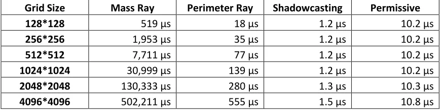
Table 3: Mean running times of our algorithm implementations in environment 2
Grid Size Mass Ray Perimeter Ray Shadowcasting Permissive
128*128 519 μs 18 μs 1.2 μs 10.2 μs
256*256 1,953 μs 35 μs 1.2 μs 10.2 μs
512*512 7,711 μs 77 μs 1.2 μs 10.2 μs
1024*1024 30,999 μs 139 μs 1.2 μs 10.2 μs
2048*2048 130,333 μs 280 μs 1.3 μs 10.3 μs
4096*4096 502,211 μs 555 μs 1.5 μs 10.8 μs
Table 4: Mean running times of Doryen implementations in environment 2
Grid Size Perimeter Ray Shadowcasting Permissive
128*128 112 μs 2 μs 50 μs
256*256 356 μs 2 μs 183 μs
512*512 1,633 μs 1.9 μs 761 μs
1024*1024 8,035 μs 2 μs 3835 μs
2048*2048 33,064 μs 2.1 μs 27.9 μs
4096*4096 144,008 μs 2.3 μs 29.4 μs
While Mass Ray FOV and Perimeter Ray FOV do benefit from only having to assign
visibility statuses to cells in a small area, their running times still increase as the grid size
increases. This is because the number of rays that these algorithms cast is dependent on
the grid size and is not affected by the vision-blocking cells.
The running times of Recursive Shadowcasting and our implementation of Permissive
FOV remain constant as the size of the grid increases because the block of visible cells
which they traverse does not change. For these algorithms an arbitrarily large FOV grid
will produce almost the same running time as the smallest possible grid which is able to
contain all visible cells.
The Doryen implementation of Permissive FOV exhibits unusual behavior in this
environment. Its running time increases as the grid size increases up to 1024*1024
because it allocates and initializes an amount of memory that depends on the size of the
FOV grid. The more memory that is allocated, the larger the running time of the
algorithm becomes. However, the amount of this memory which the algorithm actually
uses depends on the number of visible cells, and so most of the memory is unused in this
At grid sizes of 2048*2048 and above the running time of Doryen Permissive FOV
decreases. We suspect that this is caused by ‘lazy allocation’, which is a technique where
a computer will only allocate or initialize memory when a program actually uses it. At
higher grid sizes the amount of unused memory is large enough for lazy allocation to
trigger, which causes a reduction in the running time of the algorithm.
Table 5: Mean running times of our algorithm implementations in environment 3
Grid Size Mass Ray Perimeter Ray Shadowcasting Permissive
128*128 908 μs 37 μs 19 μs 59 μs
256*256 4,994 μs 115 μs 56 μs 127 μs
512*512 16,758 μs 298 μs 225 μs 327 μs
1024*1024 72,343 μs 845 μs 608 μs 852 μs
2048*2048 333,513 μs 2,545 μs 2,066 μs 2,960 μs
4096*4096 1,450,916 μs 9,470 μs 7,588 μs 8,857 μs
Table 6: Mean running times of Doryen implementations in environment 3
Grid Size Perimeter Ray Shadowcasting Permissive
128*128 166 μs 351 μs 533 μs
256*256 482 μs 1,207 μs 2205 μs
512*512 1,697 μs 4,922 μs 8,305 μs
1024*1024 8,847 μs 20,103 μs 32,638 μs
2048*2048 34,033 μs 72,732 μs 115,242 μs
4096*4096 161,096 μs 306,555 μs 471,515 μs
Environment 3 was chosen specifically to make Shadowcasting and Permissive FOV
perform a large number of ray casts. Both Shadowcasting and Permissive FOV have
much worse performance when compared to Perimeter Ray FOV in this environment
than in environment 1. The more efficient cell traversal of Shadowcasting and Permissive
FOV is less effective here, as the performance of these algorithms is reduced due to the
number of rays they must cast.
The Doryen library implementations of Shadowcasting and Permissive FOV performed
very poorly here. Clearly the Doryen implementation of these algorithms is managing
rays and ray casting in an inefficient manner, as the algorithms are slower than our
implementation by a factor of up to 50. The relative difference in running time increases
From these three test cases, we can make the following conclusions:
In terms of running time Recursive Shadowcasting is the most efficient algorithm,
however Permissive FOV is competitive with it in most cases. Perimeter Ray FOV
generally performs poorly but becomes competitive with Shadowcasting and Permissive
FOV when those algorithms must cast many visibility rays. Mass Ray FOV performs
extremely poorly in all cases and is clearly not a useful FOV algorithm.
The study given in [16] is significantly affected by inefficiencies present in the Doryen
library. The Doryen implementations of FOV algorithms perform almost universally
worse than our own, sometimes by large margins, and in some cases exhibit unusual
behavior which is inconsistent with how the FOV algorithms work. While [16] would be
useful to an implementor who plans to work with the Doryen library, it is not a useful
experimental evaluation of the FOV algorithms themselves.
Existing FOV algorithms are very well suited to environments with few visible cells but
struggle when many cells are visible. The most efficient algorithms are almost
completely unaffected by the size of the FOV grid in environment 2 but have running
times which scale quadratically with grid size in environments 1 and 3. This makes sense
based on the design of Shadowcasting and Permissive FOV, as these algorithms only
scan cells which they will set to visible. As a result their performance is primarily
dependent on how many cells will be visible in an environment.
As performance is most dependent on cell visibility assignments, the algorithms do not
scale well to higher grid sizes. In realtime applications such as computer games, an
algorithm which takes even a few milliseconds to complete may have a negative impact
on the gameplay experience. In the worst-case scenario of environment 1, Recursive
Shadowcasting becomes problematic at grids of size 512*512 and would certainly be
unusable at grids of size 1024*1024 and above. A better FOV algorithm must improve
the process of assigning visibility values to cells, either by assigning fewer visibility
1.5
Correctness Issues with Recursive Shadowcasting
While developing and testing our own implementation of the Recursive Shadowcasting
algorithm, we noticed certain cases where the algorithm as described in [14] produces
incorrect output. We describe this issue and a solution below.
When Recursive Shadowcasting traverses a row of the grid, it scans all cells in that row
which intersect the area defined by its visibility rays. If a cell even just grazes a visibility
ray, it must be set to visible. However, in certain cases a visibility ray will intersect a
vision-blocking cell and become blocked. In the example provided in Figure 12, the
visibility ray on the right intersects a vision-blocking cell at point A and hence it should
not be extended beyond that point. However, the algorithm as described in [14] would
continue the ray all the way to point B and thus incorrectly set cell C to visible. It is
therefore important for an implementation of Recursive Shadowcasting to check for
intersections and handle them appropriately. In the example provided in Figure 12, when
traversing the topmost row the algorithm must stop at the cell intersecting point A,
instead of the cell intersecting point B.
Figure 12: An example of Recursive Shadowcasting producing incorrect output. The visibility rays are shown on the left. The resulting FOV output is shown in the
This error will sometimes cause a single cell to be incorrectly set to visible. To the best of
our knowledge no existing implementation of Recursive Shadowcasting addresses this
problem. This is likely because the error will only affect one vision-blocking cell which
is at the edge of a visible region, and so the error is not easily noticed.
This error can be fixed by modifying the Recursive Shadowcasting algorithm: Rows are
traversed as described in Chapter 1.3, except an additional check occurs when the final
cell of a row is reached. When the algorithm is considering the final cell, before assigning
it a visibility status, it checks if the previous cell (i.e. the second to last cell in the row) is
vision-blocking. If the previous cell is vision-blocking, then the algorithm checks if the
visibility ray intersects it, and if so the algorithm does not assign a status of visible to the
final cell, but ends its current recursive iteration. This check is not performed if the row
being scanned only includes one cell.
Note that while our example of this error uses octant 1, where the algorithm traverses by
rows from left to right, this error may occur in any octant. Because of this, this check
must be performed while calculating the FOV for the other 7 octants as well. In some
octants this traversal will be by columns instead of rows.
Adding this check to the Recursive Shadowcasting algorithm does not significantly affect
performance and ensures that the algorithm always produces correct output according to
the definition of shadowcast visibility. Our implementation of Recursive Shadowcasting
Chapter 2
2
Improving FOV Calculation
This chapter covers our first new approach to FOV calculation: an FOV algorithm based
on a compact and efficient representation of vision-blocking cells.
2.1
Grouping Vision-Blocking Cells
The FOV algorithms which we have discussed perform two essential operations:
determining which cells are visible from the source, and storing this information in the
FOV grid. For both operations, the algorithms scan the entire FOV grid and therefore
have time complexities which at best depend linearly on the number of grid cells. This
results in poor performance at large grid sizes, as the number of cells depends
quadratically on the size of the grid.
We know that each time an FOV algorithm is run the visibility status of some cells must
be different, as otherwise there would be no reason to calculate a new FOV. However, the
positions of vision-blocking cells within the grid can be expected to change infrequently,
or not at all. Therefore, a compact representation for vision-blocking cells could be
computed once and used for many FOV calculations.
We can process blocking cells in an efficient manner by grouping adjacent
vision-blocking cells. The time complexity of determining which areas are visible and which are
not will then depend on the number of vision-blocking groups, and not necessarily on the
number of individual vision-blocking cells. In most environments increasing the FOV
grid size will increase the number of vision-blocking cells but will increase the number of
vision-blocking groups by a smaller amount. Therefore, as grid size increases an
algorithm whose performance depends on the number of vision-blocking groups will
likely have better performance than an algorithm with performance depending on the
This grouping of vision-blocking cells allows us to assign visibility statuses to cells
efficiently as well. Existing FOV algorithms assign visibility status on a per-cell basis.
By grouping vision-blocking cells and computing the area of the FOV grid that the group
occludes, we can determine the visibility of a large region of the grid at once. We can
then store visibility statuses of cells in this region in whichever order we like.
This is important because, as previously discussed in Chapter 1.4, the efficiency of
algorithms which frequently access memory is affected by the CPU cache. In addition to
storing recently accessed data the CPU cache will also store data that is located nearby,
this is called spatial locality. If a program accesses memory in a manner that takes
advantage of this property of caching, it will be significantly faster, and is said to be
taking advantage of spatial locality.
Typically cells in an FOV grid will be laid out from left to right and top to bottom in
adjacent memory locations. In other words, the first row of cells in the grid would be
stored from left to right in consecutive memory locations, then the second row would be
stored immediately after, and so on. This means that if we assign visibility status to cells
by rows from left to right we will take maximal advantage of spatial locality, which will
significantly accelerate the process of writing visibility statuses to cells (see Figure 13).
Figure 13: How cells within the region occluded by one vision-blocking cell would be assigned not visible status. Cells are shown in the grid above and are shown laid out
Some existing FOV algorithms make some use of spatial locality, but only in a limited
way. Mass Ray FOV and Perimeter Ray FOV both access grid cells which intersect the
rays that they cast and so will only incidentally benefit from spatial locality when those
rays happen to intersect cells in the same order in which they are stored in memory.
Permissive FOV traverses the cells of the grid by diagonals, and so it does not
significantly benefit from spatial locality either.
Recursive Shadowcasting does take advantage of spatial locality however. As already
discussed in Chapter 1.3, Recursive Shadowcasting moves by along the cells of the grid
by rows from left to right when processing Octant 1. However, when the Recursive
Shadowcasting algorithm is mirrored on the other 7 octants the cell traversal order
changes as well (see Figure 14). For four of the eight octants the algorithm will traverse
cells by columns and will therefore not take advantage of spatial locality.
Figure 14: Cell traversal order of Recursive Shadowcasting for each octant.
Additionally, while Recursive Shadowcasting will make use of spatial locality when it
traverses by rows, this traversal will be split when the algorithm encounters vision
blocking cells and recursively calls itself. This splitting will reduce the spatial locality of
2.2
Splitting Vision-Blocking Groups into Rectangles
As shown in Figure 15, adjacent vision-blocking cells form vision-blocking rectilinear
polygonal regions. If any holes are inside of these polygonal regions, we can fill them
with vision-blocking cells without affecting the resulting FOV. A rectilinear polygon
without holes is called a simple rectilinear polygon. These simple polygons can be
dissected into rectangles. We show an FOV algorithm that can use these vision-blocking
rectangles to efficiently determine which regions of the grid are non-visible.
Figure 15: Vision blocking cells (left) being transformed into a rectilinear polygon (center), and then a set of rectangles (right).
There are many ways to partition rectilinear polygons into rectangles, but we want to do
so in a way which minimizes the number of rectangles. This is a well-studied problem
which can be solved in polynomial time. We summarize one way to partition simple
rectilinear polygons into a minimal number of rectangles, first described in [18].
All vertices of a rectilinear polygon can be separated into two categories: concave and
convex. A vertex is concave if its internal angle is 270 degrees and convex if that angle is
90 degrees (see Figure 16 (a), where concave vertices are highlighted in red). The internal
angle of a vertex is the angle inside the polygon which is formed by the two edges
touching that vertex. A horizontal or vertical line which is entirely within a rectilinear
polygon and which connects exactly two concave vertices is a chord of that polygon (see
We construct a graph based on all the chords of a given rectilinear polygon: Each chord is
a node of the graph, and chords which intersect each other are connected by an edge. All
horizontal chords can only intersect vertical chords, and vice-versa, which means the
resulting graph will be bipartite. A bipartite graph is a graph where the nodes can be
separated into two groups, such that no nodes in the same group are connected by an
edge.
We then determine a maximum independent set of the bipartite graph, which is the
largest set of nodes no two of which are adjacent to each other (see Figure 15 (c), which
shows a bipartite graph of chords with a maximum independent set highlighted in red).
The problem of finding a maximum independent set of an arbitrary graph is NP-hard,
however for bipartite graphs a maximum independent set can be found in polynomial
time, such as with an algorithm by Hopcroft and Karp [19]. The polygon is then cut
along the chords that are part of the maximum independent set, which creates the smallest
number of rectilinear polygons that do not have any chords [18] (see Figure 16 (d), which
shows only the chords that cut the polygon).
Finally, these chord-less rectilinear polygons are partitioned into rectangles using their
concave vertices. For each concave vertex, a polygon is cut along a horizontal or vertical
line which extends from that vertex to the other side of the polygon (see Figure 16 (e),
which shows these final cuts in green). The choice between horizontal or vertical is
arbitrary, either will result in the same number of rectangles. The polygons which result
from this final process will all be rectangles, and as shown in [18] it is not possible to
partition the original polygon into fewer of them.
Having grouped vision blocking cells into rectangles, we now discuss how to use them to
calculate the FOV. Of the four corner points of a rectangle, two are relevant to
determining the visible space from a given FOV source. We refer to these two points as
the relevant points of a rectangle. The relevant points of a rectangle are the two points
which are farthest apart from each other, among all points which are not occluded behind
that rectangle (see Figure 17). Rays traced from each relevant point away from the FOV
source define the boundary between space which is occluded behind the rectangle, and
space which is not. The area between, but not including, both rays and the visible faces of
a rectangle is all space which is not visible because of that rectangle.
Figure 17: Rays cast from relevant points for two separate source positions. The area occluded by the rectangle is darkened. Two corners of the rectangle are occluded on the left, while only one is on the right. Relevant points are highlighted
in red.
We use rectangles to represent groups of vision-blocking cells instead of other more
complex polygons because rectangles are the only convex polygons which can be
accurately represented on a grid. Convex polygons are useful for representing
vision-blocking cells because, as we have shown, they can easily be processed to determine
2.3
Storing Rectangles in a Quadtree
Vision-blocking rectangles need to be stored in a data structure that allows us to process
them efficiently. We must use a data structure which allows us to represent rectangles
within 2D space. Such data structures are called spatial data structures. The spatial data
structure we have chosen to use is the quadtree [20].
Each node of a quadtree represents a region of the FOV grid and it contains all rectangles
that intersect that region. The quadtree has a parameter L that bounds the minimum
number of rectangles that must intersect the region represented by a node that would
force that region to be split into four quadrants of the same size. The first node of a
quadtree represents the entire grid and is referred to as the root node. If more than L
rectangles are within the grid, the grid is split and the root is given four child nodes which
each represent a quadrant of the grid (see Figure 18). If a node represents a region of the
grid that intersects more than L rectangles, that node is given 4 children each representing
one quadrant of the region represented by the node. Nodes are added to the quadtree and
regions are split into smaller regions until all regions intersect at most L rectangles.
A node which has children is referred to as an internal node, and a node with no children
is a leaf node. Rectangles are stored within leaf nodes; each internal node stores its four
child nodes. It should be noted that a rectangle can be contained within multiple leaf
nodes, as it can intersect more than one leaf node's region.
![Figure 1: An example of FOV in a game with simple 2D graphics [1].](https://thumb-us.123doks.com/thumbv2/123dok_us/1893959.1247648/10.612.111.540.543.699/figure-example-fov-game-simple-d-graphics.webp)