Flexible Compact High-Order FD-FD Algorithm for Computing Mode Fields of Microwave Waveguides with Regular and Reentrant Corners

Flexible Compact High-Order FD-FD Algorithm for Computing

Mode Fields of Microwave Waveguides with Regular

and Reentrant Corners

Sin-Yuan Mu and Hung-Wen Chang*

Abstract—We present a highly accurate frequency-domain finite-difference algorithm for computing mode field solutions of microwave waveguides with regular and reentrant corners. Based on FBS (Fourier-Bessel series)-derived 3-by-3 compact coefficients, our method allows for a flexible layout of the 2-D uniform grids so that distance from the waveguide boundaries to the adjacent unknowns can be arbitrary. Fourth to sixth-order convergent rates of the proposed coefficients are verified by resonance-frequency error analysis for rectangular microwave waveguides for both TE/TM polarizations. We also study the first four Neumann/Dirichlet eigenvalues of the L-shaped MW-WGs calculated by the flexible scheme, and the Neumann results are reported for the first time. Although our results achieve sixth-order accuracy for analytic modes, the sixth-order of accuracy is about one and a third for both fundamental TE and TM modes due to singularity around the reentrant corner.

1. INTRODUCTION

In the past seventy years, researchers had tried various specific techniques to increase the numerical accuracy for modeling a physical waveguide structure with sharp boundary corners, such as H-shaped waveguides, L-shaped waveguides, and waveguides with fin line like a metal knife. Tracing the history, the concept of particular treatment for domain around those corners can be dated back to Motz’s work in 1947 [1]. Motz applied circular harmonics (like-FBS) expansion to obtain better finite-difference (FD) coefficients near the vertices of a reentrant corner and those of a metal knife edge. Around these points, mild and strong singularities occur. Such electromagnetic (EM) fields are related to meromorphic functions [2, 3]. It is strange that most researches focused just on vertices of PEC wedges and had missed possible improvement over the classical 5-point and 9-point FD coefficients for Helmholtz equation in uniform region. In authors’ own view, there are two possible reasons for this. On one hand, conventional frequency-domain finite-difference (FD-FD) methods cannot handle structures with complex geometry, so more people worked on finite element method (FEM) to better treat arbitrary PEC boundaries. On the other hand, finite-difference time-domain (FD-TD) algorithms, unlike FD-FD methods, without having to invert huge sparse matrices, had enjoyed much popularity for complex and large physical problems. As the memory size gets larger and the CPU became faster in the late twentieth century, frequency-domain methods become plausible as they are better suited for high-Q structures and for those frequency-domain phenomena. It was until Hadley’s work (2002) [4] (and independently by Chang and Mu (2010) [5]) that FBS-based technique for grids inside a 2-D uniform region were available. Hadley also derived coefficients for points near dielectric interface, and even for points near dielectric corner through tedious algebraic manipulation [6]. However, rates of convergence for Hadley’s numerical modal indices were less than he had expected, and the reasons were not given in his papers. We will discuss this

Received 18 February 2019, Accepted 24 April 2019, Scheduled 27 April 2019 * Corresponding author: Hung-Wen Chang ([email protected]).

point in detail in subsequent paragraphs. The remedy for solving problems with Dirichlet/Neumann singular boundary by FD-FD and FEM has been proposed by Magura et al. (2017) [7], but it requires much additional computational effort to subtract the singular field from the whole modal fields.

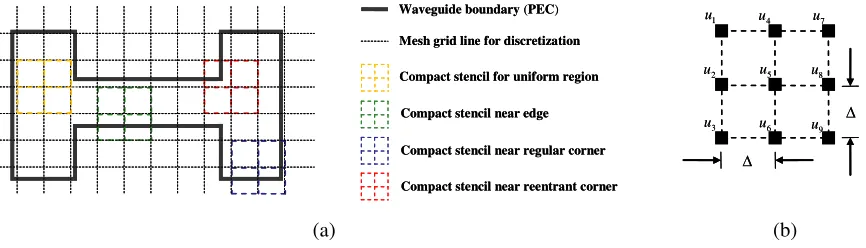
In this paper we take a deep look into the FD-FD method for analyzing microwave waveguide (MW-WG) with regular and reentrant corners made of perfect electric conductors (PEC). Fig. 1 shows an H-shaped MW-WG with the FD-FD grid layout where the FD-mesh lines are represented by dashed lines. EM fields are sampled on mesh line intersections. Some mesh lines meet with the PEC boundary, but others may not. For example, when the width to height ratio of a rectangular MW-WG is not an integral ratio, the bordering field points are not located exactly on or half-a-grid spacing from the PEC boundary. Hence we need high-order customized FD coefficients for these special nodes near boundary edges and corners. Otherwise, it will lead to less accurate simulation results. Four types of such 3-by-3 stencils are also shown in Fig. 1. All FD formulations in this paper adopt the variable order illustrated in the right part of Fig. 1. We will systematically discuss effects of mesh offsets (distance of border grids from the nearby PEC walls) on the simulation accuracy. Our goals are to maintain, under the compact-coefficient framework, high-order accuracy in discretizing Helmholtz equation for both interior grids and those near PEC boundaries with a flexible grid layout.

1 u

2 u

3 u

4 u

5 u

6 u

7 u

8 u

9 u Δ

Δ

Compact stencil near edge

Compact stencil near regular corner

Compact stencil near reentrant corner Waveguide boundary (PEC)

Mesh grid line for discretization

Compact stencil for uniform region

1 u

2 u

3 u

4 u

5 u

6 u

7 u

8 u

9 u Δ

Δ

Compact stencil near edge

Compact stencil near regular corner

Compact stencil near reentrant corner Waveguide boundary (PEC)

Mesh grid line for discretization

Compact stencil for uniform region

(a) (b)

Figure 1. (a) FD-FD mesh layout for an H-shaped MW-WG. (b) A compact 3-by-3, 9-point stencil with numbered nodal fields is given. The grid size for the uniform stencil is Δ.

We will discuss our proposed FBSE-based flexible compact coefficients in FD-FD methods for points near boundary edges, regular corners, and reentrant corners. The effectiveness of the proposed coefficients is verified by local field error analysis and TE/TM modal index computation of a rectangular MW-WG. And for the reentrant corner, it is verified by examining first four Dirichlet/Neumann eigenvalues of an L-shaped WG. Final numerical results of our algorithm demonstrate sixth-order accuracy for analytic modes, but the order of convergence is lowered to about one and a third/two and two third for modes with mild singularity around the reentrant corner.

2. EM FIELDS NEAR LOCAL WEDGES

To compute mode field solutions we may choose Hz component for transverse electric (TE) modes

(Ez ≡ 0) or Ez for transverse magnetic (TM) modes (Hz ≡ 0) [8]. Both Hz and Ez satisfy the

Helmholtz equation given by Eq. (1), where ∇2

t is the transverse Laplacian, and ξ is the transverse

wavenumber. Let the operating angular frequency be ω, and let the mode propagation constant be β. Thenξ2=k2−β2, wherek=ω√μ0ε, withεandμ0 being the permittivity and free-space permeability,

respectively. Note that the waveguide cutoff frequency fc is proportional to the cutoff wavenumber ξ

(sinceβ ≡0).

∇2

t +ξ2u= 0, fc= ₂ξc_π, u≡

Hz, TE

Ez, TM . (1)

can be well approximated by a truncated Fourier-Bessel series (FBS) for both TE and TM cases.

u(ρ, φ) =a0J0(ξρ) + M

m=1

Jm(ξρ) [amcos (mφ) +bmsin (mφ)].(FBS) (2)

On the surface of the perfect electric conductor (PEC) all tangential electric field components should be zero. In the mathematical setup, the scalar function u(ρ, φ, z) representing Hz/Ez satisfies the

Neumann boundary condition (NBC) for a TE case and the Dirichlet boundary condition (DBC) for a TM case. Hence, the particular solutions of Eq. (1) near a PEC wedge shown in Fig. 2 are expressed as Eqs. (3a)–(3b) [9].

u(ρ, φ) =

⎧ ⎪ ⎪ ⎪ ⎪ ⎨ ⎪ ⎪ ⎪ ⎪ ⎩

a0J0(ξρ) + ∞

m=1

aνmfνcm(ρ, φ), TE

∞

m=1

bνmfνsm(ρ, φ), TM

, 0≤φ≤θ0. (3a)

f_νc_m(ρ, φ) =Jνm(ξρ) cos (νmφ)

f_νs_m(ρ, φ) =Jνm(ξρ) sin (νmφ)

, νm= mπ_θ

0 , m∈N.

(3b)

In Eq. (3b),Nindicates the set of natural numbers. Boundary conditions and asymptotic behaviors of all EM components near a PEC wedge of an MW-WG are summarized in Table 1, where all expressions are in terms of local cylindrical coordinates defined in Fig. 2. In Table 1,∂ρu and∂φu represent partial

derivatives of functionuwith respect toρandφ. Note that EM field characteristics near the wedge are dominated by its included angleθ0. When θ0 ≤π, all EM components are continuous and finite at the

vertex. However, mild singularity may still exist at that point unlessθ0takes the form ofπ/n, n∈N [9].

For example, considering the case θ0 = 2π/3, the first TM asymptotic term of u(ρ, φ) is proportional

to ρ3/2, and thus the field itself (Ez) and its first derivative (Eρ and Hφ) are continuous and finite at

the vertex, but its second derivative diverges.

PEC

φ ρ

0

φ= 0

φ θ=

Figure 2. Illustration of a boundary wedge made of perfect electric conductor (PEC) with the included angle denoted byθ0. The cylindrical coordinate system is centered at the wedge vertex.

Table 1. Boundary conditions and asymptotic behaviors of EM components near a PEC wedge of a MW-WG (as shown in Fig. 2).

Transverse Expressions Asymptotic Form Comments on the Limit Value Components TE (u≡Hz,Ez≡0) TM (u≡Ez,Hz≡0) (asρ→0) (asρ→0)

Eφ ξ−2(−¯z ∂_ρu) ξ−2−jβ ρ−1∂_φu A ρπ/θ0−1cos (πφ/θ₀)

Divergent if θ0> π.

Singular when θ0=π/n,

n∈N. Hρ ξ−2(−jβ ∂ρu) ξ−2σ ρ¯ −1∂_φu B ρπ/θ0−1cos (πφ/θ₀)

Eρ ξ−2z ρ¯ −1∂_φu ξ−2(−jβ ∂_ρu) C ρπ/θ0−1sin (πφ/θ₀) Hφ ξ−2−jβ ρ−1∂φu ξ−2(−σ ∂¯ _ρu) D ρπ/θ0−1sin (πφ/θ₀)

B.C.s*

Ez= 0 Automatically satisfying

u(ρ, φ= 0) = 0 u(ρ, φ=θ0) = 0

*B.C.s: boundary conditions. Eρ= 0 ρ−1∂_φu(ρ, φ= 0) = 0

ρ−1_{∂φu(ρ, φ=θ0) = 0}

*Parameter definitions:

3. COMPACT FD-FD ALGORITHMS

Although high-order FD-FD solver may be obtained using non-compact coefficients, they lead to matrices with wider bandwidth which is undesirable due to increased storage and computational costs. A compact 9-point stencil with numbered nodal fields is shown in Fig. 2. The general expression of FD-like algebraic relation for such a stencil is given by Eq. (4), where the interested central fieldu5 is

related to the weighted sum of the immediate surrounding nodal fields.

u5 = 9

m=1, m=5

Wmum =wu,

w= [ W1 W2 W3 W4 W6 W7 W8 W9 ],

u= [ u1 u2 u3 u4 u6 u7 u8 u9 ]T.

(4)

If the nodal field um is located outside the computation domain, the associated coefficient Wm is set to be zero. Compact 3-by-3 stencils enclosing a horizontal or a vertical boundary PEC are discussed in the subsequent sections.

3.1. Coefficients for Uniform Region (UR)

Based on [4] and [5], the sixth-order accurate coefficients for uniform region are given by Eq. (5) (LFE-9). The acronym LFE represents local field expansion.

u5 =W0−1W+(u2+u4+u6+u8) +W0−1W×(u1+u3+u7+u9), W0 =4 (J0W++J0sW×), W+=J4s, W×=J4.(LFE−9)

(5)

In Eq. (5), Ji = Ji(Vt), and J_is = Ji√2Vt (i = 0,4), where Vt = ξΔ, which is the normalized transverse wavenumber.

3.2. Coefficients for Boundary Edge (θ0 =π)

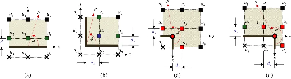
In Figs. 3(a)–3(d) we show four 9-point stencil grid layouts near PEC boundaries. The black squares indicate interior nodes. The green squares and blue ones indicate nodes near edges and near regular corners, respectively. The red squares indicate nodes near reentrant corners. The black crosses indicate nodes outside computation domain. The red circles are vertices of reentrant corners. The offset for the (a) case isd(=tΔ) whereasdx(=txΔ) anddy(=tyΔ) are horizontal and vertical offsets for the other three cases. When 0≤t <1, PEC edges alter the uniform-region coefficients for both TM and TE cases. When t = 0, the case for TM polarization is trivial, and the 4th-order accurate coefficients and the 6th-order accurate ones for Neumann boundary conditions have been proposed in Eq. (40) of [10] and in Eq. (53) of [11], respectively. Evaluating ui ((ρi, φi), i= 1,2,4,5,7,8) by Eq. (6), the truncated

version of Eqs. (3a)–(3b) for the caseθ0=πleads to Eqs. (7a)–(7b) for TE modes and to Eqs. (8a)–(8b)

for TM modes. In Eqs. (7a)–(7b), subscripts e of ue,ae, and be stand for edge. The subscripts N/D

indicate Neumann/Dirichlet BCs. ue = [ u1 u2 u4 u5 u7 u8 ]T, which is the nodal field vector

near edge. wTE

e andwTMe are the weighted coefficient vector to relate u5 to ue for TE and TM modes.

Note thatwTE_e and w_eTM are functions of the offset d.

u(ρ, φ) =

⎧ ⎪ ⎪ ⎪ ⎪ ⎨ ⎪ ⎪ ⎪ ⎪ ⎩

a0J0(ξρ) + M

m=1

amJm(ξρ) cos (mφ), TE

M

m=1

bmJm(ξρ) sin (mφ), TM

, 0≤φ≤π. (6)

PN

FN

ae=

ue u5

ρ x 1 u 2 u 3 u 4 u 5 u 6 u 8 u φ 7 u 9 u y y d x d ρ x 1 u 2 u 3 u 4 u 5 u 6 u 8 u φ 7 u 9 u y y d x d y ρ x 1 u 2 u 3 u 4 u 5 u 6 u 7 u 8 u 9 u

φ dy

x d y ρ x 1 u 2 u 3 u 4 u 5 u 6 u 8 u φ d 7 u 9 u

(a) (b) (c) (d)

Figure 3. Illustration of 9-point stencils near PEC boundaries. (a) Stencil for edge (0< φ < π). (b) Stencil for a regular corner (0 < φ < π/2). (c) Stencil for a reentrant corner (Type I with one node removed) (0< φ <3π/2). (d) Stencil for reentrant corner (Type II with two nodes removed).

PN=

ci_jJ_ji

, ci_jJ_ji Jj(ξρi) cos (j φi), i= 1,2,4,7,8, j= 0,1,2, . . . , M,

FN=

c5_jJ_j5

, ae= [ a0 a1 a2 · · · aM ]T.

(7b)

PD

FD

be=

ue u5

⇒u5=wTMe ue, weTM=FDP−_D1.(EGLFE−TM) (8a)

PD=

si_jJ_ji

, si_jJ_jiJj(ξρi) sin (j φi), i= 1,2,4,7,8, j= 1,2, . . . , M,

FD=

s51J15 s52J25 s53J35 · · · s5_MJ_M5

, be= [ b1 b2 b3 · · · bM ]T.

. (8b)

Considering the simplest case that t = 0, we may simplify Eqs. (7a)–(7b) (EG LFE-TE formulation) as Eq. (9), where W0, W+, and W× are given by Eq. (5). The coefficients given by Eq. (9) can be

equivalently obtained by imposing even symmetry condition (alongy= 0) on those coefficients defined in Eq. (5) for uniform region.

u5 =W0−1W+(u2+ 2u4+u8) +W0−1W×(2u1+ 2u7).(EG LFE-TE for t= 0) (9)

In principle we need all, up to the eighth order, FBS terms to maintain the accuracy of compact coefficients. The local field formulation achieves 8th-order accuracy, and hence FD-discretized Helmholtz equation may enjoy a 6th-order global accuracy (since discretized Helmholtz equation is divided by Δ2). Once in a while we may use fewer terms to achieve same level of accuracy because of structure symmetries as in the case of the uniform region where we only need FBS terms with orders lower than 5 [5].

3.2.1. Local Error Analysis for Edge Grids

Near a PEC edge (denoted as EG) an exact solution of Eq. (1) for the settings given by Fig. 3(a) is expressed as:

ψEG(x, y) =

cos (qy)e−jpx, TE

sin (qy)e−jpx, TM , p=γξ, andq=

1−γ21/2ξ . (10)

In Eq. (10),γis defined as the ratio ofp(tangential wavenumber component) toξ. ψEGis viewed as the

superposition of two opposite evanescent waves in y direction when |γ|>1. The analytic value of the central fieldua5 isψEG evaluated atx= 0 andy=tΔ.The corresponding numerical value un5 is defined

as the weighted sum ofψEGevaluated at the coordinates of surrounding nodal fields according to Eq. (4).

Nλ(= 2π/Vt). Similar techniques for local error analysis have been proposed in previous researches [12, 13]. Corresponding curves are shown in Figs. 4(a)–4(c) and Figs. 5(a)–5(c).

LRE(Nλ, γ, t)u n 5 −ua5

ua5

. (11)

Considering those figures, observations based on LRE analysis are summarized here.

3.2.2. I. Offset Effects

We are surprised to learn that LRE is quite sensitive to the normalized offset. The differences between the minimum and maximum LREs are from 2 to 5 orders for both TE cases (Figs. 4(a)–4(b)) and TM cases (Figs. 5(a)–5(b)). For TE cases, the optimized points are neart= 0.5 andt= 0, but for TM cases, the optimal choices are around t= 0.5 andt= 1. The convergent rate is about 8th-order whent= 0.5 and lower for other offsets. Hence, the optimal choice of offset may be around half-a-grid spacing.

(a) (b) (c)

Figure 4. Local relative errors (LRE) of edge grids using EG LFE-TE (Eqs. (7a)–(7b)) stencils as functions of (a) transverse sampling density (Nλ) (b) normalized offset (t), and (c) normalized tangential

wavenumber (γ =p/ξ). (Neumann boundary conditions are imposed.).

(a) (b) (c)

Figure 5. Local relative errors (LRE) of edge grids using EG LFE-TM formulation (Eqs. (8a)–(8b)) as functions of (a) transverse sampling density (Nλ), (b) normalized offset (t), and (c) normalized

tangential wavenumber (γ =p/ξ). (Dirichlet boundary conditions are imposed.).

3.2.3. II. Angular Spectrum Effects

Effects on spatial angular spectrum dependency are shown in Fig. 4(c) and Fig. 5(c). We see that the overall LREs remain small for propagating plane waves (when γ < 1) and increase rapidly when

3.3. Coefficients for Regular Corner (θ0=π/2)

A compact stencil near regular (right-angled) PEC corner is shown in Fig. 3(b). Between the vertex and central node, an offsetdx(=txΔ) anddy(=tyΔ) lie in the horizontal and vertical directions. When

0 ≤tx < 1 and 0≤ty <1, PEC corner coefficients are adjusted for both TM and TE cases. For TE case, when tx= 1 or ty = 1, the situation is reduced to the edge case discussed in Section 3.2. For TM case, if tx = 0 or ty = 0, then the situation can be ignored as the unknowns on the PEC corner/edge are zeros. Local fields near a regular PEC corner (denoted as PEC-CR) are given by:

u(ρ, φ) =

⎧ ⎪ ⎪ ⎪ ⎪ ⎨ ⎪ ⎪ ⎪ ⎪ ⎩

a0J0(ξρ) + M

m=1

a2mJ2m(ξρ) cos (2mφ), TE M

m=1

b2mJ2m(ξρ) sin (2mφ), TM

, 0≤φ≤π/2. (12)

Referring to Fig. 3(b) we may obtain the PEC-CR compact coefficientswTE

c and wTMc with following:

RN

GN

ac =

uc u5

⇒u5 =wTEc ue, wcTE=GNR−_N1.(CRLFE−TE) (13a)

RD

GD

bc =

uc u5

⇒u5 =wTMc uc, wcTM=GDR−D1.(CRLFE−TM) (13b)

Submatrices are defined in Eq. (14a) and Eq. (14b). RN=

ci2jJ2ij

, ci2jJ2ij J2j(ξρi) cos (2j φi), i= 4,7,8, j= 0,1,2, . . . , M,

GN=

J05 c52J25 c54J45 · · · c52MJ25M

, ac= [ a0 a2 a4 · · · a2M ],

(14a)

RD=

si2jJ2ij

, si2jJ2ij J2j(ξρi) sin (2j φi), i= 4,7,8, j= 1,2, . . . , M.

GD=

s52J25 s54J45 s56J65 · · · s52MJ25M

, bc= [ b2 b4 b6 · · · b2M ].

(14b)

3.3.1. Local Error Analysis for Regular Corner

Exact solutions of local field near a PEC-CR (Fig. 3(b)) can be expressed as products of standing plane waves as shown below:

ψCR(x, y) =

cos (px) cos (qy), TE

sin (px) sin (qy), TM , p=γξ, andq =

1−γ21/2ξ . (15)

The analyticua5 isψCRevaluated atx=txΔ andy =tyΔ.Numerical valueun5 is just the weighted sum

of ψCR evaluated at u4, u7, u8. The weighting factors wTEc and wTMc are given by Eqs. (13a)–(13b).

For simplicity, we only consider the case when tx = ty. Computed local relative errors for PEC-CR

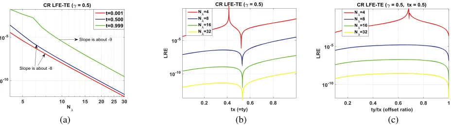
are presented in Figs. 6(a)–6(c) for the TE cases and in Figs. 7(a)–7(c) for the TM cases. As we can see from Figs. 6–7, local errors behave quite distinctively between the two polarizations. As shown in Fig. 6(c) and in Fig. 7(c), minimum LREs occur when the ratioty/tx is around 1.

3.4. Coefficients for Reentrant Corner

There are two distinct grid layouts near a PEC reentrant corner (denoted as PEC-RC) which are shown in Figs. 3(c)–3(d). For the first type only one nodal field, i.e., u3, is outside the computation

domain whereas the second type has two outside nodes u3 and u6. The offset parameters are denoted

by dx(= txΔ) and dy(= tyΔ). When tx = 1 and ty = 1, as illustrated in Fig. 3(c), uniform region

(a) (b) (c)

Figure 6. Plots of local relative errors (LRE) of CR LFE-TE against (a) transverse sampling density (Nλ), (b) normalized offset (t) and (c) offset ratio (tx/ty). (Neumann boundary condition).

(a) (b) (c)

Figure 7. Local relative errors (LRE) of CR LFE-TM as functions of (a) transverse sampling density (Nλ), (b) normalized offset (t) and (c) offset ratio (tx/ty). (Dirichlet boundary condition).

coefficients. Exact FBS-based solutions of the local field near a PEC reentrant corner as illustrated in Figs. 3(c)–3(d), for both TE and TM cases, are given by [9]:

u(ρ, φ) =

⎧ ⎪ ⎪ ⎪ ⎪ ⎨ ⎪ ⎪ ⎪ ⎪ ⎩

a0J0(ξρ) + M

m=1

a2m/3J2m/3(ξρ) cos (2mφ/3), TE M

m=1

b2m/3J2m/3(ξρ) sin (2mφ/3), TM

, 0≤φ≤3π/2. (16)

Here PEC-RC compact coefficients w_RCITE, wTM_RCI, wTE_RCII and wTM_RCII are computed by following expressions:

QN,I

VN

ar =

uRCI u5

⇒u5 =wTERCIuRCI, wTERCI=VNQ−_{N, I}1, (RCLFE−TE−I) (17a)

QD,I

VD

br =

uRCI u5

⇒u5 =wTMRCIuRCI, wTMRCI=VNQ−_N.I1, (RCLFE−TM−I) (17b)

QN, II

VN

ar =

uRC II u5

⇒u5 =wTERCIIuRCII, wTERCII=VNQ−_{N, II}1 , (RCLFE−TE−II) (17c)

QD,II

VD

br =

uRCII u5

where QN,I=

ci_jJ_ji

, ci_j J_jiJj(ξρi) cos (j φi), i= 1,2,4,5,6,7,8, j= 0,1,2, . . . , M,

VN=

J05 c52/3J 5 2/3 c

5 4/3J

5

4/3 · · · c 5 2M/3J

5 2M/3

, ar=

a0 a2/3 a4/3 · · · a2M/3

_T

,

(18a)

QD,I=

si_jJ_ji

, si_jJ_ji Jj(ξρi) sin (j φi), i= 1,2,4,5,6,7,8, j = 1,2, . . . , M,

VD=

s5_2/3J_2/35 s5_4/3J_4/35 s52J25 · · · s52M/3J 5 2M/3

, br=

b2/3 b4/3 b2 · · · b2M/3

_T

.

(18b)

Note that stencil matrices QD,I and matrix QN,I in Eqs. (18a) and (18b) are for PEC-RC type I

configuration. Type II PEC-RC matrix QD,II is obtained from QD,I with the last row removed. The

same rule applies toQN,II.

3.4.1. Local Error Analysis for Reentrant Corner

PEC-EG and PEC-CR structures support (standing) plane wave solutions given by Eq. (10) and Eq. (15), but such solutions do not always exist for PEC-RC shown in Fig. 3(c) and Fig. 3(d). For local error analysis, an exact solution near a PEC-RC,ψRC(x, y), is defined in Eq. (19) by truncating

Eq. (16) at the thirtieth term, and all weighting factors are set to be one.

ψRC(ρ, φ)

⎧ ⎪ ⎪ ⎪ ⎪ ⎪ ⎨ ⎪ ⎪ ⎪ ⎪ ⎪ ⎩

29

m=0

J2m/3(ξρ) cos (2m φ/3), TE

30

m=1

J2m/3(ξρ) sin (2m φ/3), TM

. (19)

The analyticua5 isψRC evaluated atx=txΔ, y=tyΔ.Numerical value un5 is just the weighted sum of ψRC evaluated at u4, u7, u8 for Type I-II reentrant corners. For simplicity, we only consider the case

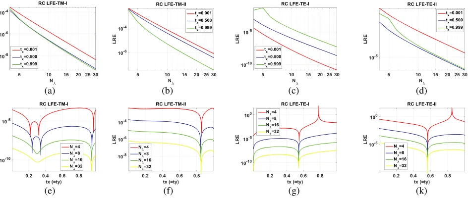
when tx =ty. In Figs. 8(a)–8(d) LREs of RC LFE-TM and RC LFE-TE are plotted against transverse

sampling density (Nλ).In Figs. 8(e)–8(h) they are plotted against the normalized offset (tx/ty). Type

II errors are in general somewhat larger, and the orders of convergent rate are less than those of Type I.

(a) (b) (c) (d)

(e) (f) (g) (k)

4. NUMERICAL SIMULATION OF MW-WG MODES

4.1. Simulation of a Rectangular Waveguide

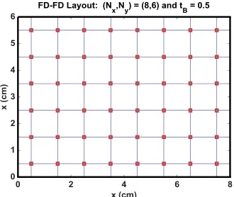
We now turn to the global error study of our proposed LFE-base compact stencils. First, we look at the rectangular waveguide with a flexible mesh layout as illustrated in Fig. 9. Boundary field points next to the left, right, and top PEC walls are fixed at half-a-grid spacing leaving varying grid spacing at the bottom PEC. The normalized bottom offset is denoted by tB. With a fixed waveguide dimension we

continuously change the number of sampling points, Nx, in the x-direction. Computed global relative errors (RErr) of numerical cutoff frequencies versusNx are plotted in Figs. 10(a)–10(c) for TE10, TE01,

and TE11 modes. The results for TM11, TM21, and TM12 modes are shown in Figs. 11(a)–11(c). From

these plots we see that relative TE mode errors are more sensitive to the normalized bottom offset parametertB than those of TM cases. Overall we observed that the minimum error (with a 6-th order accurate convergent rate) occurs when tB equals 0 or 0.5. Convergent rates for the other two cases, tB= 0.25 and tB= 0.75, are only at 5th-order.

Figure 9. Flexible FD-mesh layout for the rectangular MW-WG.

N x

5 10 15 20 25

RErr

10-10 10-8 10-6 10-4

Rectangular MW-WG (TE 10Mode)

tB=0.50 tB=0.25 tB=0.75 tB=0

N x

5 10 15 20 25

RErr

10-10 10-8 10-6 10-4

Rectangular MW-WG (TE 01Mode)

tB=0.50 tB=0.25 tB=0.75 tB=0

N x

5 10 15 20 25

RErr

10-10 10-8 10-6 10-4

Rectangular MW-WG (TE 11Mode)

tB=0.50 tB=0.25 tB=0.75 tB=0

(a) TE Mode10 (b) TE Mode01 (c) TE Mode11

Figure 10. (Rectangular MW-WG) Global relative errors (RErr) of numerical cutoff frequencies for (a) TE10, (b) TE01, and (c) TE11 modes as functions of thex-directional sampling points Nx.

4.2. Simulation of an L-Shaped Waveguide

(a) TM Mode11 (b) TM Mode21 (c) TM Mode12

Figure 11. (Rectangular MW-WG) Global relative errors of numerical cutoff frequencies for (a) TM11,

(b) TM21, and (c) TM12 modes as functions of thex-directional sampling points.

Waveguide boundary (PEC)

Grid line

Interior node for uniform stencil

Node near boundary edge

Node near regular corner

Node near reentrant corner (type I)

Node near reentrant corner (type II)

1

U

t Δ

1

R

t Δ

3

R

t Δ

3

U

t Δ

B

t Δ

L

t Δ

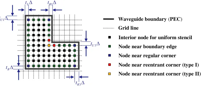
Figure 12. Flexible FD-mesh layout for the L-shaped (made of three unit squares) MW-WG. The number of sampling points in xdirection for the upper left square Nx1 = 5.

SettingL= 1,the number of x-directional sampling points of the upper-left square (Nx1) is related to

the grid spacing Δ asNx1+tL+tR1−1 =L/Δ.OnceNx1 is given, the grid size Δ and the other three

parameters tU1, tB, and tR3 are determined from it. In Fig. 12, LFE-9 formulation is applied to the

nodes marked as black squares. Compact stencils for green and blue nodes are respectively EG LFE stencils (Eqs. (7a)–7(b) and Eqs. (8a)–(8b)) and CR LFE stencils (Eqs. (13a)–(13b) and Eqs. (14a)– (14b)). Stencils for the red and yellow nodes, which are the immediate neighboring grids of the reentrant corner, are adjusted based on Eqs. (17a)–(17d) and Eqs. (18a)–(18b). First ten Dirichlet eigenvalues of Eq. (1) for L-shaped domain can be found in [14], and their square roots serve as the reference values of TM-polarized cutoff frequencies. Later on, a whopping 1001 significant digits of the first Dirichlet eigenvalue for L-shaped domain was given by Jones (2017) [15], where he obtained the result by combing the FHM algorithm [16] with infinite precision floating point arithmetic.

(a) (b)

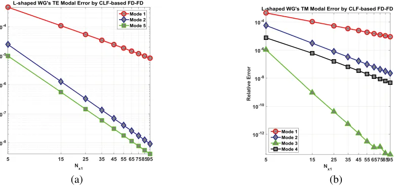
Figure 13. (L-shaped MW-WG) Global relative errors (RErr) of numerical cutoff frequencies for (a) TE modes (left) and for (b) TM modes (right).

convergent rate (about 2.7). Resonant transverse wavelengths of higher order modes are shorter than those of lower order modes, so the singularity field of a higher-order mode attenuates much more as it propagates away from the reentrant corner. Thus, the relative errors of higher order modes are smaller than those of lower ones except for analytic cases as listed in Table 2 and Table 3. When Nx1 = 95

(about 27 thousands variables), our results give 5 significant digits for the fundamental TE/TM modes, and 7 to 8 digits for higher-order singular modes. Nevertheless, the overall convergence orders for the proposed LFE-based FD algorithm are still better than the results reported in [17] where the modified FEM is applied. Since the singularity field spreads out from the reentrant corner, the effect is globalized instead of being localized [7]. This intrinsic limitation impedes numerical performance of solving mode field problems with incoming PEC wedges, or with dielectric corners with high index contrasts, by all FD-FD and FEM algorithms.

Table 2. Numerical TM results (DBC) of the L-shaped MW-WG by LFE-based FD-FD solver.

No. Exact Value ofξ[22] ξ(Nx1= 95) RErr* CO* Comments

1 3.1047904 3.1047620280375 9E-06 1.33 This mode is dominated byρ2/3term. This is the strongest singular mode.

2 3.8983652 3.8983653775956 2E-08 2.66 This mode is dominated byρ4/3term and suffers from less singularity.

3 Exact√2π 4.4428829381582 3E-14 6 No singularity. u(x, y) =Asin (πx) sin (πy).

4 5.4333673 5.4333674078062 4E-09 2.64 High-order singular mode suffers from less singularity.

*RErr: relative error; CO: convergent order

Table 3. Numerical TE results (NBC) of the L-shaped MW-WG by LFE-based FD-FD solver.

No. Reference Value ofξ(N_x1= 500) ξ(N_x1= 95) RErr CO Comments

1 1.21475 1.2147403776183 8E-06 1.33 This mode is dominated by aρ2/3 term and suffers from the strongest singularity. 2 1.8799019 1.8799019744744 2E-08 2.71 This mode is dominated by aρ4/3term. 3 Exactπ 3.1415926539879 1.3E-10 6 No singularity. u(x, y) = Acos (πx) +

Bcos (πy).

5. CONCLUSIONS

Traditional FD schemes are limited in two ways. First, the mesh pattern is rectangular and thus is unsuitable for problems with curved boundaries. Second, the accuracy of FD-FD is optimized when square uniform mesh is implemented resulting in arbitrary grid offsets near PEC walls for general waveguide structures. In this paper, we present a flexible LFE-based FD-FD algorithm for simulating complex microwave waveguides with regular and reentrant corners. We maintain the highest possible orders of accuracy for all customized compact stencils near the PEC borders. The cutoff frequency convergence rates for various rectangular waveguides are always 5th- to 6th-order accurate for both types of polarizations.

In the simulation of a typical L-shaped MW-WG, the resonant Neumann frequencies are reported for the first time. We also demonstrate: (a) The local errors of FBSE-based coefficients for these specialized stencils are at least of 5th order; (b) The order of accuracy of the fundamental WG cutoff frequency is one and a third for both the TE mode and TM mode; (c) Numerical results for higher-order singular modes converge faster than those for the fundamental modes; and (d) The convergent rate for analytic modes achieves sixth-order as expected. Compared with the 8-th order accuracy of the uniform cell (local-error), the loss of accuracy for those customized cells near a PEC wall/corner is due to the loss of grid symmetry in the presence nearby PEC boundary. The overall resonant frequencies are not calculated with expected performance of our proposed LFE-based compact stencils. The loss of global accuracy in these cases is entirely due to the singular field emanating from the reentrant corner.

ACKNOWLEDGMENT

We are grateful for the support of the Ministry of Science and Technology of the Republic of China under the contracts (MOST 107-2221-E-11-045).

REFERENCES

1. Motz, H., “The treatment of singularities of partial differential equations by relaxation methods,”

Quart. Appl. Math., Vol. 4, 371–377, 1947.

2. Arfken, G. B. and H. J. Weber, Mathematical Methods for Physicists, Elsevier Academic Press, 2005.

3. Antipov, Y. A. and V. V. Sivestrov, “Diffraction of a plane wave by a right-angled penetrable wedge,”Radio Science, Vol. 42, RS4006, 2007.

4. Hadley, G. R., “High-accuracy finite difference equations for dielectric waveguide analysis I: Uniform regions and dielectric interfaces,”Journal of Lightwave Technology, Vol. 20, No. 7, 1210–1218, 2002. 5. Chang, H.-W. and S.-Y. Mu, “Semi-analytical solutions of the 2-D homogeneous Helmholtz equation by the method of connected local fields,”Progress In Electromagnetics Research, Vol. 109, 399–424, 2010.

6. Hadley, G. R., “High-accuracy finite difference equations for dielectric waveguide analysis II: Dielectric corners,” Journal of Lightwave Technology, Vol. 20, No. 7, 1219–1231, 2002.

7. Magura, S., S. Petropavlovsky, S. Tsynkov, and E. Turkel, “High-order numerical solution of the Helmholtz equation for domains with reentrant corners,”Applied Numerical Mathematics, Vol. 118, 87–116, 2017.

8. Pozar, D. M., Microwave Engineering, John Wiley & Sons, Inc., 2012.

9. Fox, L. and R. Sankar, “Boundary singularities in linear elliptic differential equations,” J. Inst. Math. Applic., Vol. 5, 340–350, 1969.

10. Singer, I. and E. Turkel, “High-order finite difference methods for the Helmholtz equation,”

Comput. Methods Appl. Mech. Engrg., Vol. 163, 343–358, 1998.

12. Mu, S.-Y. and H.-W. Chang, “Theoretical foundation for the method of connected local fields,”

Progress In Electromagnetics Research, Vol. 114, 67–88, 2011.

13. Mu, S.-Y. and H.-W. Chang, “Dispersion and Local-Error Analysis of Compact LFE-27 Formula for Obtaining Sixth-Order Accurate Numerical Solutions of 3D Helmholtz Equation,” Progress In Electromagnetics Research, Vol. 143, 285–314, 2013.

14. Yuan, Q. and Z. He, “Bounds to eigenvalues of the Laplacian on L-shaped domain by variational methods,” Journal of Computational and Applied Mathematics, Vol. 233, 1083–1090, 2009.

15. Jones, R. S., “Computing ultra-precise eigenvalues of the Laplacian within polygons,”Advances in Computational Mathematics, Vol. 43, 1325–1354, 2017.

16. Fox, L., P. Henrici, and C. Moler, “Approximations and bounds for eigenvalues of elliptic operators,”SIAM J. NUMER. ANAL., Vol. 4, No. 1, 89–102, 1967.