Matrix Method for Far-Field Calculation Using Irregular Near-Field Samples for Cylindrical and Spherical Scanning Surfaces

Matrix Method for Far-Field Calculation Using Irregular Near-Field

Samples for Cylindrical and Spherical Scanning Surfaces

Mohamed Farouq*, Mohammed Serhir, and Dominique Picard

Abstract—A matrix method which takes into account the probe positioning errors in cylindrical and spherical near-field (NF) measurement techniques is proposed. The near-field irregularities made impossible the determination of the cylindrical or spherical wave expansion from the measured data using classical techniques based on 2D Discrete Fourier Transformation (2D-DFT) in cylindrical case (CC) and orthogonality properties in spherical case (SC). The irregularities can be randomly distributed but known and the matrix method expresses the linear relation between the measured near-field and the corresponding cylindrical or spherical modal expansion coefficients. Once the coefficients of the cylindrical and the spherical wave expansions are known the far-field of the antenna under test (AUT) is easily determined. Accuracy of the matrix method is numerically studied as a function of the irregularities magnitude and for different noise levels (data Signal to Noise Ratio). Also, experimental results have shown the efficiency of the proposed technique.

1. INTRODUCTION

The NF techniques offer the possibility to test antennas in a controlled environment for highly accurate antenna characterization. The measured near-field data are then transformed to calculate the AUT far-field. Indeed, the far-field (FF) is assessed through the expansion of the AUT radiated field in terms of modes, i.e., a complete set of solutions of the vector wave equation. Plane, cylindrical, or spherical waves are used and the type of the expansion selected for the field representation is determined according to the near-field scanning surface. The development of planar wave expansion is presented in [1]. The cylindrical formalism is detailed in [2] and the spherical one in [3].

In many circumstances it may not be possible to directly measure the near-field over a regular grid according to a canonical surface (cylindrical or spherical) due to probe positioning errors. These irregularities can be randomly distributed but known (laser tracker). In this situation the application of the modal expansion method based on 2-D DFT in the CC and the orthogonality properties in the SC to determine the FF from the measured NF is not possible. Here we propose a new method to determine the antenna far-field from non-regular NF data collected over a cylindrical or a spherical surface.

The existing solutions in the literature are based on interpolating the irregular NF data into regular grid [4–10]. However, the application of these methods in the case of 3-D irregularities is not possible. As an alternative to the interpolation methods, the irregular NF data is used to assess equivalent electric and magnetic sources [11–16]. These equivalent sources are determined by solving the inverse radiation problem solution of the integral equations relating the sources and the measured NF. Once these equivalent electric and magnetic currents are fully defined, the AUT far-field is determined by reradiating the equivalent sources at far distances. The equivalent sources method can handle NF data measured over irregular but a priori informations about the AUT to characterize (AUT dimensions, location, type...) are needed.

Received 9 April 2015, Accepted 2 June 2015, Scheduled 9 June 2015

* Corresponding author: Mohamed Farouq ([email protected]).

More recently, an interesting approach is presented in [17–19]. The method is derived from a spherical wave expansion (SWE) of the AUT radiated field. The spherical waves are expanded in propagating plane waves with similar properties to equivalent currents method. It determines the far-field of the antenna using near-far-field data measured over an irregular grid. However, the time calculation is the drawback of this method. To overcome this disadvantage a multilevel fast multipole method is used in [20] to perform matrix vector products and accelerate the resolution of the linear system.

In [21], we have proposed a matrix method for antenna plane wave spectrum calculation using irregularly distributed near-field data. The far-field calculation of the matrix method has been compared with the results of the equivalent currents method in front of the AUT. In this paper, we present the matrix method that uses non-regularly spaced near-field samples distributed randomly nearby a cylindrical or a spherical surface for the AUT far-field calculation in all directions. The irregular measured field is expanded in terms of cylindrical or spherical waves and the matrix method uses a matrix notation to describe the linear relation between the measured field and the cylindrical and spherical wave coefficients.

The paper is organized as follows. The mathematical formulation of the matrix method is described in Section 2. In Section 3, numerical investigations of the matrix method are presented using infinitesimal dipoles array. Then, a base station antenna is measured in the cylindrical measurement setup and standard gain horn antenna is measured in the spherical measurement setup for the matrix method experimental validation. Finally, concluding remarks are outlined in Section 4.

2. MATHEMATICAL FORMULATIONS

We propose a method to compute the modal expansion coefficients in order to calculate the AUT radiation FF pattern from an irregularly distributed NF samples in both cylindrical and spherical scanning surfaces. This section details the mathematical formulation of the proposed method for cylindrical and spherical cases. Throughout this paper, exp(jωt) time dependence is suppressed in all the E-field expressions.

2.1. The Cylindrical Formalism

Let us consider a measurement cylinder of radius r0, outside the minimum cylinder of radius rmin surrounding an arbitrary AUT. The measured NF is described in cylindrical coordinates system (r0,φ,

z). Over the measurement cylinder, the tangential components of the electric field can be presented [2] as a truncated summation of cylindrical waves.

E_φre(r0, φp, zq) ≈

Ncyl

n=−N_cyl

M

m=1

bn(kzm)nk m z kr0 H

(2)

n (αmr0)−an(k_zm)∂H

(2)

n ∂r (α

m_r

0)

ejnφp_e−jkmz zq_Δk

z(1)

E_zre(r0, φp, zq) ≈

Ncyl

n=−N_cyl

M

m=1

bn(kmz )α m

k H

(2)

n (αmr0)ejnφpe−jk

m z zq_Δk

z (2)

where, 0 ≤ φp ≤ 360◦ with P = (φmax − φmin)/Δφ + 1 and zmin ≤ zq ≤ zmax with Q = (zmax−zmin)/Δz + 1. Δφ and Δz are respectively the sampling steps in φ and z directions. The number of cylindrical modes is calculated using Ncyl =int(krmin) +n1 withn1 ∈N, the typical value of n1 is comprised between 5 and 10, int is the integer function andrmin is the radius of the minimum cylinder circumscribing the AUT. −π/Δz ≤km_z ≤ π/Δz, with M = (kzmax −kzmin)/Δkz+ 1, H

(2)

n is

the Hankel function of the second kind of ordern with αm =k2_−(km

z )2, an(kz) and bn(kz) are the cylindrical wave coefficients. To calculate the cylindrical wave coefficients an(kz) andbn(kz) we can use a 2D-DFT [2].

Otherwise, let us notice that (1) and (2) can be expressed in a linear matrix form as:

E_φre(r0, φp, zq) =Are1,φan(kzm) +Are2,φbn(kmz )

E_zre(r0, φp, zq) =Are2,zbn(kzm)

where,

an(k_zm) = ⎛ ⎜ ⎝

a−Ncyl(k1z)

.. .

aNcyl(kzM)

⎞ ⎟

⎠ bn(k_zm) = ⎛ ⎜ ⎝

b−Ncyl(kz1)

.. .

aNcyl(kMz )

⎞ ⎟

⎠ (4)

Are1,φ = ⎛

⎝ c1.._.,1 . . ._{. . .} c1,MN.._.

cP Q,1 . . . cP Q,MN ⎞

⎠_{, A}re

2,φ= ⎛

⎝ d1.._.,1 . . ._{. ..} d1,MN.._.

dP Q,1 . . . dP Q,MN ⎞ ⎠

Are2,z = ⎛

⎝ w1.._.,1 . . ._{. ..} w1,MN.._.

wP Q,1 . . . wP Q,MN ⎞

⎠ (5)

with, N = 2Ncyl+ 1

⎧ ⎪ ⎪ ⎪ ⎪ ⎪ ⎪ ⎪ ⎪ ⎪ ⎨ ⎪ ⎪ ⎪ ⎪ ⎪ ⎪ ⎪ ⎪ ⎪ ⎩

c1,1=−

∂H₋(2)_Ncyl ∂r

α1r0

ej(−Ncylφ1−k1zz1)

cP Q,1=−

∂H₋(2)_Ncyl ∂r

α1_r 0

ej(−NcylφP−k1zzQ)

c1,MN=−

∂H_Ncyl(2) ∂r

αMr0

ej(Ncylφ1−kMz z1)

cP Q,MN=−

∂H_Ncyl(2) ∂r

αMr0

ej(NcylφP−kzMzQ) ⎧ ⎪ ⎪ ⎪ ⎪ ⎪ ⎪ ⎪ ⎨ ⎪ ⎪ ⎪ ⎪ ⎪ ⎪ ⎪ ⎩

d1,1=−Ncylk 1

z

kr0 H

(2)

−Ncyl

α1r0

ej(−Ncylφ1−k1zz1)

dP Q,1=−Ncylk 1

z

kr0 H

(2)

−Ncyl

α1r0

ej(−NcylφP−k1zzQ)

d1,MN=Ncylk

M z

kr0 H

(2)

Ncyl

αMr0

ej(Ncylφ1−kzMz1)

dP Q,MN=Ncylk

M z

kr0 H

(2)

Ncyl

αMr0

ej(NcylφP−kMz zQ) ⎧ ⎪ ⎪ ⎪ ⎪ ⎪ ⎪ ⎪ ⎨ ⎪ ⎪ ⎪ ⎪ ⎪ ⎪ ⎪ ⎩

w1,1= α 1

k H−(2)Ncyl

α1_r 0

ej(−N_cylφ1−k1zz1)

wP Q,1 = α 1

kH−(2)Ncyl

α1_r 0

ej(−N_cylφP−kz1zQ)

w1,MN = α

M

k HN(2)cyl

αMr0

ej(Ncylφ1−kMz z1)

wP Q,MN = α_kMH_N(2)_cylαMr0

ej(NcylφP−kMz zQ)

(6)

E_φre= ⎛

⎝ Eφ

(r0, φ1, z1) .. .

Eφ(r0, φP, zQ) ⎞

⎠ _Ere

z =

⎛ ⎝ Ez

(r0, φ1, z1) .. .

Ez(r0, φP, zQ) ⎞

⎠ (7)

As an extension, we generalize the matrix method to deal with the irregular distributed NF data which can due to the position errors caused by the probe displacement. Consequently, the irregular grid provides from a slightly modified regular grid. The Near-Field (NF) data are collected over a 3-D grid defined by (rminir ≤rlir ≤rmaxir ,φirmin ≤φirl ≤φirmax and zminir ≤zirl ≤zirmax), for 1 ≤l≤L, with L is the number of measured points.

In this situation (irregular NF), (3) can be written as follows:

Eir_φ r_lir, φ_lir, z_lir=Air1,φan(kzm) +A2ir,φbn(kzm)

Eir_z r_lir, φir_l , z_lir=Air2,zbn(kmz )

(8)

where,

Air1,φ= ⎛

⎝ c1.._.,1 . . . c_{. ..} 1,MN.._.

cL,1 . . . cL,MN ⎞ ⎠_{, A}ir

2,φ = ⎛

⎝ d1.._.,1 . . . d_{. ..} 1,MN.._.

dL,1 . . . dL,MN ⎞ ⎠

Air2,z= ⎛

⎝ w1.._.,1 . . . w_{. ..} 1,MN.._.

wL,1 . . . wL,MN ⎞

⎧ ⎪ ⎪ ⎪ ⎪ ⎪ ⎪ ⎪ ⎪ ⎪ ⎨ ⎪ ⎪ ⎪ ⎪ ⎪ ⎪ ⎪ ⎪ ⎪ ⎩

c1,1=−

∂H₋(2)_Ncyl ∂r

α1rir1

ej(−Ncylφlir−k1zzir1 )

cL,1 =−

∂H₋(2)_Ncyl ∂r

α1rir_Lej(−NcylφirL−k1zzLir)

c1,MN =−

∂H_Ncyl(2) ∂r

αMr1ir

ej(N_cylφir₁−kM_z zir₁ )

cL,MN =−∂H (2)

Ncyl

∂r

αMrir_Lej(NcylφirL−kMz zLir)

⎧ ⎪ ⎪ ⎪ ⎪ ⎪ ⎪ ⎪ ⎪ ⎨ ⎪ ⎪ ⎪ ⎪ ⎪ ⎪ ⎪ ⎪ ⎩

d1,1= −Ncylk 1

z

krir

1 H

(2)

−Ncyl

α1rir1

ej(−Ncylφ1ir−k1zz1ir)

dL,1= −Ncylk 1

z

krir L H

(2)

−Ncyl

α1rir_Lej(−NcylφirL−k1zzLir)

d1,MN = Ncylk

M z krir 1 H (2) Ncyl

αMrir1

ej(Ncylφir1−kMz z1ir)

dL,MN = Ncyl_krirkzM L H

(2)

Ncyl

αMrir_Lej(NcylφirL−kMz zLir)

⎧ ⎪ ⎪ ⎪ ⎪ ⎪ ⎪ ⎪ ⎨ ⎪ ⎪ ⎪ ⎪ ⎪ ⎪ ⎪ ⎩

w1,1 = α 1

kH−(2)Ncyl

α1r1ir

ej(−Ncylφ1ir−kz1zir1)

wL,1 = α 1

k H−(2)Ncyl

α1rir_Lej(−NcylφirL−k1zzLir)

w1,MN = α

M

k H

(2)

Ncyl

αMrir1

ej(Ncylφir1−kMz z1ir)

wL,MN = α_kMHN(2)cyl

αMr_Lirej(NcylφirL−kzMzirL)

(10)

E_φir = ⎛ ⎜ ⎝

Eφ(rir1, φir1 , z1ir) .. .

Eφ(rir_L, φir_L, z_Lir) ⎞ ⎟

⎠ E_zir= ⎛ ⎜ ⎝

Ez(r1ir, φir1, z1ir) .. .

Ez(r_Lir, φir_L, z_Lir) ⎞ ⎟

⎠ (11)

Solving (3) or (8) the coefficientsan(kz) andbn(kz) are determined and the FF is computed in the

spherical coordinates:

Eθ(r, θ, φ) = −j2ksinθe

−jkr r

n=+N_cyl

n=−N_cyl

jnbn(kcosθ)ejnφ (12)

Eφ(r, θ, φ) = −2ksinθe

−jkr r

n=+N_tr

n=−Ntr

jnan(kcosθ)ejnφ (13)

2.2. The Spherical Formalism

In the case of spherical coordinates (r0, θ, φ) and outside the minimum sphere of radius rmin circumscribing the AUT, the spherical wave expansion of the radiated electric field is expressed in terms of truncated series of spherical vector wave functions [3] as

E(r0, θ, φ)≈ √k

η

2

s=1

Nsph

n=1

n

m=−n

QsmnFsmn(4) (r0, θ, φ) (14)

where,η=0/μ0is the intrinsic admittance, r0 the radius of measurement sphere,Qsmnthe spherical wave coefficients, andFsmn(4) the power normalized spherical wave functions of the outward propagating fields. The expressions of Fsmn(4) are developed in [3]. The truncation numberNsph = int(krmin) +m1 depends on the antenna dimensions and the operating frequency and m1 ∈ N with a typical value comprised between 5 and 10. Introducing an index l such thatl = 2n(n+ 1) +m−1 +s, (14) can be written in the following form

E(r0, θ, φ)≈ √k

η Lmax

l=1

QlFl(4)(r0, θ, φ) (15)

where,Lmax= 2Nsph(Nsph+2). In the classical case of a regular meshing on a spherical surface of radius

these coefficients are known, the electromagnetic field can be evaluated everywhere outside the minimum sphere of radiusrmin enclosing the AUT. Equation (15) can be expressed in a matrix form as

E_θre(r0, θh, φp)

E_φre(r0, θ_h, φp)

=

F_θre F_φre

Q (16)

where, Eθ and Eφ are the tangential components of E(r0, θ, φ)

F_θre = ⎛ ⎜ ⎝

F1θ(r0, θ1, φ1) . . . F_Lθ_max(r0, θ1, φ1) ..

. . . . ...

F1θ(r0, θN_θ, φ2(Nφ−1)) . . . F_Lθ_max(r0, θN_θ, φ2(Nφ−1)) ⎞ ⎟ ⎠

F_φre = ⎛ ⎜ ⎝

F1φ(r0, θ1, φ1) . . . F_Lφ_max(r0, θ1, φ1) ..

. . . . ...

F1φ(r0, θN_θ, φ2(Nφ−1)) . . . F_Lφ_max(r0, θN_θ, φ2(Nφ−1)) ⎞ ⎟

⎠ (17)

E_θre = ⎛ ⎜ ⎝

Eθ(r0, θ1, φ1) .. .

Eθ(r0, θN_θ, φ2(Nφ−1)) ⎞ ⎟

⎠ E_φre= ⎛ ⎜ ⎝

Eφ(r0, θ1, φ1) .. .

Eφ(r0, θN_θ, φ2(Nφ−1)) ⎞ ⎟

⎠ (18)

Q =

⎛ ⎝ Q.._.1

QLmax ⎞

⎠ (19)

where, 0 ≤ θh ≤ 180◦ with Nθ = (θmax− θmin)/Δθ + 1 and 0 ≤ φp ≤ 360◦ with 2(Nφ −1) = (φmax−φmin)/Δφ+ 1. Δθand Δφare respectively the sampling steps inθ andφ directions.

In the case of measured field over an irregular grid, the spherical wave coefficients assessment using the orthogonality properties are not possible. The spherical wave coefficients are in this case determined by solving a system of linear equations. The Near-Field (NF) data are collected over a 3-D grid defined by (rminir ≤rirl ≤rmaxir , θirmin ≤ θlir ≤θmaxir and φirmin ≤ φirl ≤ φirmax), for 1 ≤l ≤ Lsph, with Lsph is the number of measured points. Equation (16) can be re-expressed as follow:

E_θir(rir_l , θ_lir, φir_l )

E_φir(rir_l , θ_lir, φir_l )

=

F_θir F_φir

Q (20)

where,

F_θir = ⎛ ⎜ ⎜ ⎝

F1θ(r1ir, θir1, φir1) . . . FLθ_max(r1ir, θ1ir, φir1) ..

. . .. ...

F1θ(rirL_sph, θLir_sph, φirL_sph) . . . FLθ_max(rirL_sph, θLir_sph, φirL_sph) ⎞ ⎟ ⎟ ⎠

F_φir = ⎛ ⎜ ⎜ ⎝

F1φ(r1ir, θir1 , φir1) . . . F_Lφ_max(r0ir, θir1, φir1 ) ..

. . .. ...

F1φ(rLir_sph, θirL_sph, φirL_sph) . . . FLφmax(rLirsph, θirLsph, φirLsph)

⎞ ⎟ ⎟

⎠ (21)

E_θir = ⎛ ⎜ ⎜ ⎝

Eθ(r1ir, θ1ir, φir1) .. .

Eθ(rLirsph, θirLsph, φirLsph)

⎞ ⎟ ⎟

⎠ E_φir = ⎛ ⎜ ⎜ ⎝

Eφ(r1ir, θ1ir, φir1) ..

.

Eφ(rLirsph, θirLsph, φirLsph)

⎞ ⎟ ⎟

⎠ (22)

Once the spherical wave coefficients Ql are determined the FF is expressed as

E(r, θ, φ) = √k

η

1

√

4π e−jkr

kr Lmax

l=1

where, K_l(4) is the FF radiation pattern developed in [3].

We have developed a Matlab routine solving (3) and (8) for the cylindrical formalism and a Matlab routine solving (16) and (20) for the spherical formalism. These routines are based on the use of LSQR method [22]. In the following study, we aim at evaluating the efficiency of the matrix method for far-field assessment in different situations.

3. RESULTS

3.1. Procedure

The matrix method is tested using three examples comprising numerical simulation and experimental measurements results. In the first example the NF data are computationally generated using analytical expression of an infinitesimal dipoles array. In the second example NF data result from a base station antenna measured in the Supelec cylindrical near-field measurement setup. In the last example, the matrix method is tested using NF data issued from a standard gain horn antenna measured in the spherical near-field system.

The accuracy of the matrix method is evaluated by comparing the reference co-polar FF (Eref) and the co-polar FF resulting from the matrix method (Ecalc) in both cylindrical and spherical configurations. The error(%) is defined as bellow:

error(%) = 100

θ,φ

|Ecalc(θ, φ)−Eref(θ, φ)|2

θ,φ

|Eref(θ, φ)|2

(24)

A parametric study of the matrix method is carried out using an array composed of 40 infinitesimal dipoles. The near-field is calculated analytically over an irregular grid generated as follows. First, a regular near-field grid is defined using constant Δz, Δφ for the cylindrical configuration and constant Δθ, Δφ for the spherical configuration. Then, a weighted random function Ran varying between −1 and +1 are added to each measurement position to create a randomly distributed near-field which is controlled by the weighting factorχ. Finally, we consider for a given measurement radiusr0 a random weighting function Ranr varying between 0 and χr to control the irregularities over the measurement distance. This procedure is summarized in (25).

CC ⎧ ⎪ ⎪ ⎨ ⎪ ⎪ ⎩

rir_l(p,q)=r0+Ranrχr

φir_l(p,q)=pΔφ+Ranφχφ

z_lir_(p,q)=qΔz+Ranzχz

SC ⎧ ⎪ ⎪ ⎨ ⎪ ⎪ ⎩

rir_l(h,p)=r0+Ranrχr

θir_l(h,p)=hΔθ+Ranθχθ

φir_l(h,p)=pΔφ+Ranφχφ

(25)

The proposed parametric study includes 3D irregularities. For a constant measurement radius the irregularities can be corrected using 2-D interpolation algorithms as presented in [10]. These interpolation algorithms can not deal with the irregularities over (r,φ,z) for the cylindrical configuration and (r, θ, φ) for the spherical configuration. In our study the effect of the irregularities over the measurement radius is outlined. Also, the signal to noise ratio is an important parameter to take into account. For this reason, a Matlab function (AWGN: Additive White Gaussian Noise) is used to reduce the SNR of the near-field data used for the far-field calculation resulting from the matrix method.

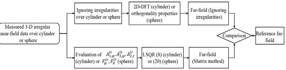
Figure 1. Validation procedure of the matrix method.

3.2. The Cylindrical Case

3.2.1. Numerical Results

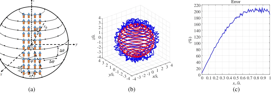
Let us consider the AUT composed of 4×10z-polarized infinitesimal dipoles array placed in theyz-plane (Fig. 2(a)). The array dipoles areλ/2 spaced along they and zdimensions with a constant excitation. The cylindrical NF measurement surface is centered on the axis of the AUT. The field is collected over the cylinder r0= 3λ, 0≤φ≤2π, Δφ= 10◦,zmax=−zmin= 10λand Δz=λ/2.

For this dipoles array, we create an irregular near-field data for different χr values. We aim at

determining the cylindrical wave coefficients (CWC) an andbn consideringNcyl=int(krmin) + 6 = 10 and the FF radiation pattern of each near-field distribution resulting from each χr while ignoring

the irregularities using 2D-DFT. These far-field results are compared with the reference one and the evaluated error is presented in Fig. 2(c). In Fig. 2(c) we present the behavior of the error as a function of the weighting factor χr. It is seen that the error increases as the weighting factor increases. In the

situation of χr/λ = 0.01 the difference between the reference FF and the calculated one is negligible

compared with the case ofχr/λ= 1.

As an example we consider χr = λ, χφ = 2◦ and χz = λ/10 for detailed comparisons. The

cylindrical wave coefficients are calculated while taking into account the irregularities. To do this, the matrix method is used forNcyl = 10. For the same irregular NF data (χr=λ,χφ= 2◦ andχz =λ/10),

the cylindrical wave coefficients are calculated using a 2D-DFT (irregularities are ignored). The results

6 4 2 0 -2 -4 -6 -6 -4 -2 0 2 4 8 10

-2 0 2

-6 -4 4

-10 6

-8

6

0 0.1 0.2 0.3 0.4 0.5 0.6 0.7 0.8 0.9 1 0

20 40 60 80 100 120 140 160

(a) (b) (c)

x/λ

y/λ

z

/

λ

Error

(%)

x r/λ

0 20 40 60 80 100

10 20 30 40 50 60 70 80 90 100 110

10 20 30 40 50 60 70 80 90 100 110

(a) (b) (c)

-10

-8

-6

-4

-2

0

2

4

6

8

10

n

-10

-8

-6

-4

-2

0

2

4

6

8

10

n

-10

-8

-6

-4

-2

0

2

4

6

8

10

n

b n(k z)(W 1/2) b n(k z)(W 1/2) b n(k z)(W 1/2)

-1 -0.75 -0.5-0.25 0 0.25 0.5 0.75 1 k z/k

-1 -0.75-0.5-0.25 0 0.25 0.5 0.75 1 k z/k

-1 -0.75-0.5-0.25 0 0.25 0.5 0.75 1 k z/k

Figure 3. Cylindrical wave coefficientsbn(kz) as a function of nandkz/k. (a) Regular grid, (b) matrix method, (c) ignoring irregularities, for the dipoles array.

-40 -30 -20 -10 0 10 20 30 40 50

Reference

Matrix method

Ignoring irregularities χ /λ=0.01

Ignoring irregularities χ /λ=1

Error = 104%

Error = 0.36%

-20 -10 0 10 20 30 40 50

Reference

Matrix method

20 30 40 50 60 70 80 90 100

3 4 5 6 7 8 9 10 11 12

Cylindrical modes=7 Cylindrical modes=10

-180 -150 -120 -90 -60 -30 0 30 60 90 120 150 180

φ( )o

(a) (b) (c)

Magnitude (dB) Magnitude (dB)

(%)

0 20 40 60 80 100 120 140 160 180

θ( )o

SNR (dB)

Co-polar (θ = 90 )o

Co-polar (φ = 0 )o

Error

Error = 1.8%

Error = 3.1%

Error = 4.3%

Error = 105%

r r

Ignoring irregularities χ /λ=0.01

Ignoring irregularities χ /λ=1

r r

Figure 4. (a), (b) Co-polar FF component in the two main planes for the dipoles array and (c) error versus SNR for the dipoles array.

are compared with the cylindrical wave coefficients issued from regular NF data for Ncyl = 10. This

comparison is carried out in Fig. 3. As it is seen, the cylindrical wave coefficients issued from regular and irregular NF data are visually identical for the matrix method. The use of 2D-DFT is no more acceptable for the far-field calculation (cylindrical wave coefficients) in the case of irregular NF data. Theancoefficients are negligible compared withbncoefficients since the AUT is polarized inz-direction.

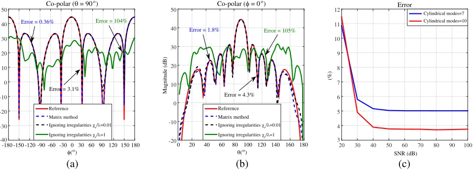
In Figs. 4(a), (b), we compare the reference FF, the FF obtained using the matrix method with

χr/λ = 1 and the calculated one when we ignore to take into account the irregularities in two cases χr/λ= 0.01 andχr/λ= 1 in bothθ= 90◦andφ= 0◦ cut planes. It is seen from Fig. 5(a) and Fig. 5(b) that the matrix method results present an excellent agreement with the reference radiation pattern in both directions (error = 0.36% inθ= 90◦and error = 1.8% inφ= 0◦). The result of the matrix method is the blue curve forχr/λ= 1. If the irregularities are not taken into account in the case ofχr/λ= 0.01 (black curve), the errors are low (error = 3.1% inθ= 90◦ and error = 4.3% inφ= 0◦). However, when we have considered a high irregularities level (χr/λ= 1), results are completely altered and the errors are equal to error = 104% in θ= 90◦ and error = 105% inφ= 0◦.

Fig. 4(c) present the error values as a function of the signal to noise ratio of the near-field data. It is seen from Fig. 4(c) that the error function takes high values for low SNR near-field data. However, beyond the threshold of 40 dB, the error function stays stable. In the case when we decrease the number of considered modes (Ncyl= 7), the error value increases in a controlled way.

3.2.2. Experimental Results

Here we show the matrix method results for a base station antenna (Fig. 5) measured with the cylindrical near-field setup. We consider the operating frequency 1.88 GHz and the antenna dimensions are 65 cm×26 cm×7 cm.

At the first step we measure the tangential NF components over a regular grid cylinder for (−177 cm≤zmeas ≤177 cm and 0≤φmeas≤360◦) with Δz=λ/2.5 and Δφ= 11.25◦ over 3 different

cylinders of radius (rmeas = 45 cm, 49 cm and 53 cm). Then, the used NF in the matrix method is

constructed by choosing randomly the NF samples from the 3 measurement grids to compose the 3D irregular near-field data. For our investigations we useNcyl =int(krmin) + 10 = 15.

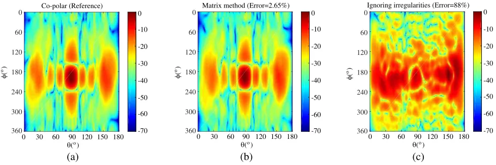
Figure 6 shows the radiation pattern comparison. The reference FF calculated using 2D-DFT for a regular cylinder with rmeas = 49 cm is presented in Fig. 6(a), the FF issued from the matrix

method using irregular grid is shown Fig. 6(b). In Fig. 6(c), the FF results from 2D-DFT of ignored irregularities NF data is presented. It can be seen that the use of the matrix method generate a good

Figure 5. The base station antenna measured in the cylindrical near-field facility.

0

60

120

180

240

300

360 -70

-60 -50 -40 -30 -20 -10 0

-70 -60 -50 -40 -30 -20 -10 0

-70 -60 -50 -40 -30 -20 -10 0

(a) (b) (c)

0 30 60 90 120 150 180

θ( )o 0 30 60 _θ90 120 150 180_{( )}o 0 30 60 _θ90 120 150 180_{( )}o

φ

( )

o

0

60

120

180

240

300

360

φ

( )

o

0

60

120

180

240

300

360

φ

( )

o

Co-polar (Reference) Matrix method (Error=2.65%) Ignoring irregularities (Error=88%)

-50 -45 -40 -35 -30 -25 -20 -15 -10 -5 0

Reference Matrix method Ignoring irregularities

Reference Matrix method Ignoring irregularities

Error = 89% Error = 1.7%

φ( )o

(a) (b)

Magnitude (dB)

θ( )o

Co-polar (θ = 90 )o Co-polar (φ = 180 )o

Error = 1.36% Error = 86%

-50 -45 -40 -35 -30 -25 -20 -15 -10 -5 0

Magnitude (dB)

0 40 80 120 160 200 240 280 320

0 20 40 60 80 100120 140 160180 360

Figure 7. Co-polar FF comparison in the two main planes for the base station antenna.

results (error = 2.65%) compared with the case of ignoring irregularities (error = 88%).

To compare the results of the matrix method and for ignored irregularities with the reference FF, we present the main FF cut planes. We calculate the error values for every comparison. Results are shown in Fig. 7(a) and Fig. 7(b). From these figures, we notice that the radiation patterns for ignored irregularities are considerably distorted (error = 86% in θ = 90◦ and error = 89% in φ = 180◦). Meanwhile, the matrix method results are consistent for the co-polarization cut planes (error = 1.36% inθ= 90◦ and error = 1.7% inφ= 0◦).

3.3. The Spherical Case

3.3.1. Numerical Results

To evaluate the effect of considering the irregularities in spherical formalism, we use the same AUT (4×10 z-dipoles) as the one considered in the previous part. The field generated by (4×10 z-dipoles) is collected over a sphere with r0 = 5λ, 0 ≤ θ ≤ 180◦, 0 ≤ φ ≤ 360◦ with Δθ = Δφ = 7.5◦. These parameters (r0, Δθ, Δφ) are used to generate the irregular NF data and the NF is exploited to calculate the spherical wave coefficients using the matrix method.

To calculate the spherical wave coefficients Ql, we consider Nsph =int(krmin) + 10 = 24. Using

4 3 2 1 0 -1 -2 -3 -4 -4 -3 -2 -1 0 1 2 3 1 2 3 4

0

-4 -3 -2 -1

4

0 0.1 0.2 0.3 0.4 0.5 0.6 0.7 0.8 0.9 1 0

20 40 60 80 100 120 140 160 180 200 220

(a) (b) (c)

x/λ

y/λ

z

/

λ

x r/λ Error

(%)

this parameter, we evaluate the FF radiation pattern of each NF data resulting from each χr while ignoring the irregularities using the orthogonality properties. These far-field results are compared with the reference one and the calculated error is presented in Fig. 8(c). It is seen that the error value grows as the weighting factor increases. Considering the case of χr = 0.01 the error between the reference FF

and the calculated one is insignificant compared with the case of χr= 1.

To demonstrate the effectiveness of the proposed method, we considerχr =λ,χθ = 2◦ andχφ= 2◦

andNsph= 24. These parameters allow us to calculate the spherical wave coefficientsQlusing the matrix

method and the orthogonality properties when the irregularities are ignored. The results are compared with the spherical wave coefficients issued from regular NF data for Nsph = 24. This comparison is

carried out in Fig. 9. As it is seen, the spherical wave coefficients issued from regular and irregular NF data using the matrix method are visually identical. The application of the orthogonality properties are not appropriate for the calculation of spherical wave coefficients (FF) in the case of irregular NF data. We compare the calculated FF using the matrix technique and the reference FF determined from classical NF to FF transformation of regular NF data collected over a spherical surface with (r0 = 5λ, Δθ = 7.5◦, Δφ = 7.5◦ and Nsph = 24). We evaluate the error between the reference FF and the

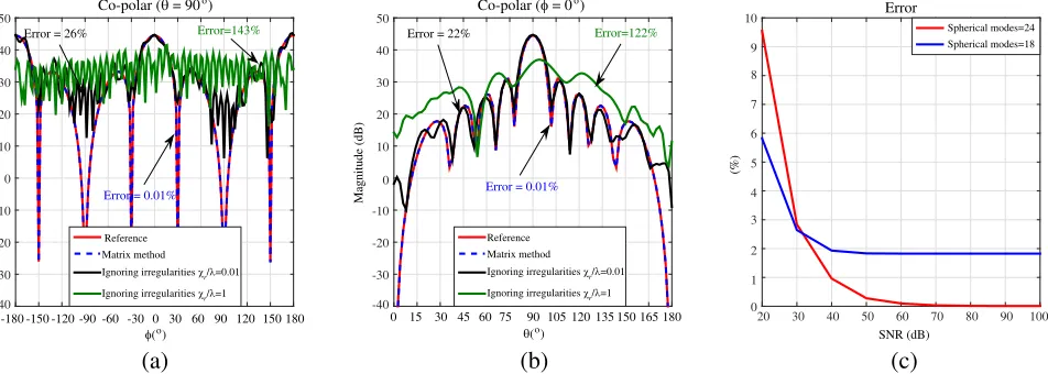
calculated ones. These are presented in Fig. 10(a) and Fig. 10(b).

As it can be seen the matrix method results present a good agreement with the reference radiation pattern (error = 0.01% in θ = 90◦ and error = 0.01% in φ = 0◦). If the irregularities are not taken into account forχr/λ= 1, this leads to high errors as it seen in Fig. 10(a) and Fig. 10(b) (green curve)

0 200 400 600 800 1000 1200 1400

× 105

0 0.5 1 1.5 2 2.5

0 1 2 3 4 5 6 7

l

(a) (b) (c)

0 200 400 600 800 1000 1200 1400

l

0 200 400 600 800 1000 1200 1400

l

|

Q

| (

W

)

l

1/2

0 0.5 1 1.5 2 2.5

|

Q

| (

W

)

l

1/2

|

Q

| (

W

)

l

1/2

× 105 × 105

N sph= 18 N sph= 24

Figure 9. Spherical wave coefficients Q as a function of l. (a) Regular grid, (b) matrix method, (c) ignoring irregularities, for the dipoles array.

20 30 40 50 60 70 80 90 100

-180 -150 -120 -90 -60 -30 0 30 60 90 120 150 180

φ( )o

(a) (b) (c)

0 15 30 45 60 75 90 105120 180

θ( )o

SNR (dB) 135 150 165

-40 -30 -20 -10 0 10 20 30 40 50

3 4 5 6 7 8 9 10

Magnitude (dB)

(%)

Co-polar (θ = 90 )o _{Co-polar (φ = 0 )}o

Error

-40 -30 -20 -10 10 20 30 40 50

Magnitude (dB)

0 Error=143%

Error = 0.01% Error = 0.01%

Error = 26% Error = 22% Error=122%

0 1 2

Reference Matrix method

Ignoring irregularities χ /λ=0.01

Ignoring irregularities χ /λ=1

r r

Reference Matrix method

Ignoring irregularities χ /λ=0.01

Ignoring irregularities χ /λ=1

r r

Spherical modes=24 Spherical modes=18

(error = 143% in θ= 90◦ and error = 122% inφ = 0◦). With ignored irregularities forχr/λ= 0.01 a slight difference is observed (error = 26% in θ= 90◦ and error = 22% in φ= 0◦).

Moreover, we are interested in studying the effect of the SNR over the calculation stability that can influence the accuracy of the matrix method. The NF data are calculated at irregular positions (rir,θir,φir) and contaminated with a controlled additive white Gaussian noise level to reduce the data signal to noise ratio. Fig. 10(c) presents the error between the reference FF and calculated one as a function of the signal to noise ratio of NF data. From Fig. 10(c), the error function takes high values for low SNR data. However, beyond the threshold of 50 dB the error function stays stable. Using less number of modes Nsph= 18 increases the error value.

3.3.2. Experimental Results

The proposed method in spherical coordinates is validated using the Supelec spherical range. The antenna used to determine the far field from 3-D irregular near-field measurements samples is a standard gain horn antenna (Fig. 11) operating at the frequency 8 GHz, the antenna waveguide dimensions are 2.3 cm×1 cm and the size of the aperture is 13 cm×9 cm.

Using the spherical range, we measure the tangential components of the horn antenna radiated NF over a regular grid (0◦ ≤ θmeas ≤ 167◦ and 0◦ ≤φmeas ≤360◦) with Δθ = Δφ= 3◦ over 3 different

spheres of radius (rmeas = 40 cm, 41 cm and 42 cm). Then, the used near-field in the matrix method is

constructed by choosing randomly the NF samples from the 3 spherical measurement grids to compose the 3D irregular near-field data. For this antenna we chose (Nsph=int(krmin) + 10 = 28).

The FF calculated using the matrix method and when ignoring the irregularities are presented in Fig. 12. The reference FF is calculated directly using a near-field to far-field transformation for the full

Figure 11. The standard gain horn antenna measured in the spherical NF facility.

0

60

120

180

240

300

360

-70 -60 -50 -40 -30 -20 -10 0

(a) (b) (c)

0 30 60 90 120 150 180

θ( )o

φ

( )

o

Co-polar (Reference) Co-polar (Matrix method Error=0.3%) Co-polar (Ignoring irregularities Error=233%)

0

60

120

180

240

300

360

φ

( )

o

0

60

120

180

240

300

360

φ

( )

o

0 30 60 90 120 150 180

θ( )o 0 30 60 _θ90 120 150 180

( )o

-90 -80

-70 -60 -50 -40 -30 -20 -10 0

-90 -80

-100

-70 -60 -50 -40 -30 -20 -10 0

-80

Reference Matrix method Ignoring irregularities

Reference Matrix method Ignoring irregularities -40

-35 -30 -25 -20 -15 -10 -5 0

φ( )o

(a) (b)

Magnitude (dB)

θ( )o

Co-polar (θ = 90 )o Co-polar (φ = 180 )o

0 60 120 180 240 300

0 30 60 90 120 150 180 -40 360

-35 -30 -25 -20 -15 -10 -5 0

Magnitude (dB)

Error = 107%

Error = 0.2%

Error = 0.1% Error = 262%

Figure 13. Co-polar FF comparison in the two main planes for the standard gain horn antenna.

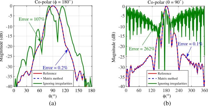
sphere situated at (rmeas= 41 cm). The error between the results from our method and the reference for the co-polarization is equal to (error = 0.3%). When we ignore the irregularities the radiation pattern is completely altered (error = 233%).

The principal cut planes comparison are shown in Fig. 13(a) and Fig. 13(b). As it can be seen, the proposed method presents a good agreement with the reference FF (error = 0.1% inθ = 90◦ and error = 0.2% in φ = 180◦). In contrast, the principal cut planes in case we ignore the irregularities shows huge difference compared to the reference pattern (error = 262% inθ= 90◦ and error = 107% in

φ= 180◦).

4. CONCLUSION

A matrix method in both cylindrical and spherical coordinates to assess the far-field of an AUT from its irregular NF samples has been presented. The proposed method employs an irregular distributed NF data nearby a cylinder or a sphere to calculate the corresponding cylindrical or spherical wave coefficients. Moreover, considering the same situation (irregular distributed NF data), the application of the classical methods (2D-DFT in CC and orthogonality properties in SC) is not possible.

With regular sampling, the use of the fast Fourier transform reduces the computational complexity of near-field to near-field or far-field transform (o(krmin)log(krmin)). However, the matrix method presents a computational complexity of ordero(krmin)3.

Numerical and experimental data are used to illustrate the effectiveness of the proposed method in both cylindrical and spherical coordinates. The numerical simulation results are performed by controlling numerically the irregularities magnitude. In contrast, to generate the experimental results we have measured in more than one corresponding cylindrical or spherical surface using respectively a base station antenna (cylindrical setup) and standard gain horn antenna (spherical setup). It has been shown that the radiation pattern of the antennas under test can be determined accurately using the matrix method. In the case when we ignore to take into account the irregular samples the radiation pattern may be strongly altered.

REFERENCES

1. Joy, E. B. and D. Paris, “Spatial sampling and filtering in near-field measurements,”IEEE Trans. Antennas Propagat., Vol. 34, No. 3, 253–261, 1972.

2. Leach, Jr., W. and D. Paris, “Probe compensated near-field measurements on a cylinder,” IEEE Trans. Antennas Propagat., Vol. 21, No. 4, 435–445, 1973.

4. Yen, J., “On nonuniform sampling of bandwidth-limited signals,” IRE Trans. Circuit Theory, Vol. 3, No. 4, 251–257, 1956.

5. Rahmat-Samii, Y. and R. Cheung, “Nonuniform sampling techniques for antenna applications,”

IEEE Trans. Antennas Propagat., Vol. 35, No. 3, 268–279, 1987.

6. Dehghanian, V., M. Okhovvat, and M. Hakkak, “A new interpolation method for reconstructing non-uniformly spaced samples into uniform ones in planar near-field antenna measurements,”IEEE Antennas and Propagation Society International Symposium, 2003, Vol. 3, 207–210, Jun. 22–27, 2003.

7. Dehghanian, V., M. Okhovvat, and M. Hakkak, “A new interpolation technique for the reconstruction of uniformly spaced samples from non-uniformly spaced ones in plane-rectangular near-field antenna measurements,” Progress In Electromagnetics Research, Vol. 72, 47–59, 2007. 8. Bucci, O. M., C. Gennarelli, and C. Savarese, “Interpolation of electromagnetic radiated fields over

a plane by nonuniform samples,” IEEE Trans. Antennas Propagat., Vol. 41, No. 11, 1501–1508, 1993.

9. Wittmann, R. C., B. K. Alpert, and M. H. Francis, “Near-field antenna measurements using nonideal measurement locations,”IEEE Trans. Antennas Propagat., Vol. 46, No. 5, 716–722, 1998. 10. Marvasti, F., Nonuniform Sampling, Theory and Practice, Kluwer, Norwell, 2001.

11. Petre, P. and T. K. Sarkar, “Planar near-field to far-field transformation using an equivalent magnetic current approach,”IEEE Trans. Antennas Propagat., Vol. 40, No. 11, 1348–1356, 1992. 12. Sarkar, T. K. and A. Taaghol, “Near-field to near/far-field transformation for arbitrary near-field

geometry utilizing an equivalent electric current and MoM,” IEEE Trans. Antennas Propagat., Vol. 47, No. 3, 566–573, 1999.

13. Taaghol, A. and T. K. Sarkar, “Near-field to near/far-field transformation for arbitrary near-field geometry, utilizing an equivalent magnetic current,” IEEE Trans. Electromagnetic Compatibility, Vol. 38, No. 3, 536–542, 1996.

14. Las-Heras, F., M. R. Pino, S. Loredo, Y. Alvarez, and T. K. Sarkar, “Evaluating near-field radiation patterns of commercial antennas,” IEEE Trans. Antennas Propagat., Vol. 54, No. 8, 2198–2207, 2006.

15. Alvarez, Y., F. Las-Heras, and M. R. Pino, “Reconstruction of equivalent currents distribution over arbitrary three-dimensional surfaces based on integral equation algorithms,”IEEE Trans. Antennas Propagat., Vol. 55, No. 12, 3460–3468, 2007.

16. Persson, K. and M. Gustafson, “Reconstruction of equivalent currents using a near-field data transformation with radome application,” Progress In Electromagnetics Research, Vol. 54, 179– 198, 2005.

17. Schmidt, C. H., M. M. Leibfritz, and T. F. Eibert, “Fully probe-corrected near-field far-field transformation employing plane wave expansion and diagonal translation operators,”IEEE Trans. Antennas Propagat., Vol. 56, No. 3, 737–746, 2008.

18. Schmidt, C. H. and T. F. Eibert, “Assessment of irregular sampling near-field far-field transformation employing plane-wave field representation,” IEEE Magazine Antennas Propagat., Vol. 53, No. 3, 213–219, 2011.

19. Qureshi, M. A., C. H. Schmidt, and T. F. Eibert, “Adaptive sampling in multilevel plane wave based near-field far-field transformed planar near-field measurements,” Progress In Electromagnetics Research, Vol. 126, 481–497, 2012.

20. Schmidt, C. H. and T. F. Eibert, “Multilevel plane wave based near-field far-field transformation for electrically large antennas in free-space or above material halfspace,” IEEE Trans. Antennas Propagat., Vol. 57, No. 5, 1382–1390, 2009.

21. Farouq, M., M. Serhir, and D. Picard, “Matrix method for antenna plane wave spectrum calculation using irregularly distributed near-field data: Application to far-field assessment,” Progress In Electromagnetics Research M, Vol. 42, 71–83, 2015.