A Joint Detection and Tracking Algorithm for Unresolved Target
and Radar Decoy
Zhiyong Song*, Fei Cai, and Qiang Fu
Abstract—Miniature Air Launched Decoy (MALD) is an electronic warfare technique for inducing an angular deception in a monopulse radar by recreating glint angular error. MALD flies cooperatively with the true target, forms unresolved group targets within the radar beam, and destroys the detection, tracking and parameter estimation of monopulse radar for the true target. In this paper, a typical scenario for one target and one decoy was discussed, and the measurement model of target and decoy based on the actual non-ideal sampling conditions was established. The joint multi-targets probability density was adopted to dynamically describe the number and state of the targets within the radar beam. Based on the original observation without threshold decision, a joint detection and tracking algorithm for unresolved target and decoy was proposed under the Bayesian framework, and the judgment of existence of jamming and the target state estimation were deduced. Simulation results showed that the proposed method enabled quick detection of the appearance of MALD and estimated the state of target with minimal delay and high precision. Stable tracking of the true target was achieved under severe jamming conditions.
1. INTRODUCTION
The miniature air launched radar decoy is a new kind of angle deception jamming [1]. The decoy flies cooperatively with true target and realistically simulates the flight envelope and echo feature of target. The characteristic difference between the target and decoy is reduced greatly, and the unresolved multiple targets are formed [2–4]. Traditional processing of monopulse radar is suitable for the case where only one target falls within the resolution unit, and when two or more targets fall into the same unit of radar beam, the echoes of them will overlap with each other, and it will cause the uncertainty of radar observation and result in a great deviation of angle measurement [5]. The towed radar decoy, air launched radar decoy, cross-eye jamming and ground-rebound jamming, which are developed from this feature, all have good angle deception effects and bring challenges to target detection, measuring and tracking. Therefore, the detection and tracking of unresolved targets are of great significance for improving the capability of anti-jamming for monopulse radar.
For the detection and tracking problem of unresolved targets in radar beam, various methods have been proposed in the literature. Some involve special antenna configuration [6], array signal processing (beamforming, space-time adaptive processing (STAP), subspace rejection, high resolution spectrum analysis) [7–12], multiple-input multiple-output (MIMO) radar [13, 14], and dual-polarization radar [15, 16]. Nevertheless, these methods require additional configuration and processing for traditional monopulse radar, and their promotion and application are limited. Other methods involve the complete utilization of standard monopulse radar system, through modifying signal and data processing algorithms and software without increasing the hardware cost. Through analyzing and extracting the characteristic variety under two situations when single target and multiple unresolved
Received 31 October 2018, Accepted 11 January 2019, Scheduled 21 January 2019
* Corresponding author: Zhiyong Song ([email protected]).
targets are in radar beam, the detection and tracking of multiple targets are implemented separately. The characteristics to detect the unresolved targets include complex monopulse ratio [17, 18], range glint [19] and sample phase error [20], and the angle estimation methods include moment estimation [21– 23] and maximum likelihood estimation [24–27]. The target detection in these methods refers to detect target multiplicity rather than the detection of presence. On the other hand, multiple target tracking methods such as joint probabilistic data association (JPDA) filter [28, 29] and multiple hypothesis tracker (MHT) [30, 31] are introduced to resolve the continuous tracking of unresolved or merged targets when the tracking interleaving occurs. However, in these multi-targets tracking methods, the unresolved targets are manly in the observation data, not in the signal, and these methods do not control signal processing. All of the above methods considered the detection and tracking of unresolved targets as two separate processes. The estimation and tracking are based on the measurement after the threshold decision, and the information loss caused by threshold detection under low signal-to-noise ratio (SNR) will seriously affect the effectiveness of the methods.
Corresponding to the separated processing of detection and tracking, the joint detection and tracking method that integrates detection processing and tracking processing has great potential to deal with unresolved targets. The rapid development of the finite set statistics (FISST) theory [32, 33] has afforded a new theoretical framework for the joint detection and tracking of a target under complex conditions using a random finite set (RFS) [34]. Some methods adopting probability hypothesis density (PHD) filter [35], labeled PHD filter [36, 37], cardinalized probability hypothesis (CPHD) filter [38], and cardinality balanced multi-target multi-Bernoulli (CBMeMBer) filters [39] were addressed to resolve the detection and tracking of unresolved targets. Unfortunately, the assumption condition of the RFS method for the detection and tracking of unresolved targets is that the targets among the unresolved group do not overlap with each other. This assumption is obviously different from the unresolved situation caused by air launched decoy; therefore, this method is not applicable. Meanwhile, the track before detect (TBD) method based on the original signal without threshold decision can obtain detection and tracking results simultaneously utilizing the motion model of target and realizing the signal accumulating according to the motion law. This kind of method can effectively avoid the information loss caused by threshold decision and improve the detection and tracking performance under low SNR. The common TBD method includes Dynamic Programming (DP) [40, 41], Hough Transform (HT) [42], and particle filter (PF) [43]. Particle filtering techniques that have the advantage of providing computational tractability are applicable under most general circumstances since there is no assumption made on the form of the density. Some methods utilizing particle filter were introduced to detect and track two closely spaced targets [44, 45], and they focused on constructing hypothesis testing for detection based on Akaike information criterion (AIC) and using particles to achieve state estimation [46, 47].
In the present study, a typical scenario of one target launching one radar decoy was used to model the unresolved target and jamming within the radar beam by analyzing the jamming process of the MALD. The joint multi-targets probability density model was used to describe the number of targets in the radar beam and their states under the Bayesian framework. The joint detecting and tracking algorithm for the target and decoy based on particle filter was designed to realize the accurate detection of jamming and stable tracking of target. The effectiveness of this algorithm was experimentally validated. The rest of this paper is organized as follows. Section 2 presents the analysis and signal model of the miniature air launched radar decoy. Section 3 presents the joint detection and tracking algorithm of unresolved targets and deduces its particle realization form, especially the existence detection of jamming and state estimation of targets. Section 4 presents the results of simulation experiments performed using the algorithm. The conclusions of the study are finally presented in Section 5.
2. SIGNAL AND JAMMING MODEL
and decoy is [48]
θ= Δθ 2
ISR2−1
ISR2+ 1 (1)
where Δθ is the angle interval between the target and decoy relative to radar. Eq. (1) shows that the greater the MALD power is, the closer the monopulse radar is to the decoy. When the radar cannot distinguish the target and decoy, their energy centers will be used as the attack point for parameter measurement and tracking and will result in loss of target. The jamming process of a typical MALD is shown in Figure 1. The target gradually deceives the beam point of monopulse radar by releasing the decoy and eventually left only the decoy in the radar beam, and the target successfully escapes from the radar beam.
(a) (b)
(c) (d)
Figure 1. The jamming process of MALD ((a) not releasing MALD, (b) just releasing MALD, (c) cooperative flying, (d) target escape form radar beam).
It can be seen form Figure 1 that there are 4 cases of target number existing during the jamming course for one target with one decoy: the target does not exist; the target exists; the target exists, but the jamming does not exist; the target and decoy both exist. Therefore, the number of targets in the radar beam at timekcan be modeled as a discrete variablemk∈ {0,1,2}, where the jamming is another “target” and therefore counts in the number of targets. During the jamming process, the changes of the target numbermk can be modeled as a Markov process, and the state transformation matrix is
Π =
π00 π01 π02 π10 π11 π12 π20 π21 π22
(2)
whereπij p(mk =i|mk−1 =j).
The state vector of target and decoy is expressed asxjk(j =T, D), whereT represents target, andD
represents decoy. In order to simplify the analysis, only two-dimensional plane is considered. Therefore, the state of single target or decoy is [xjk,x˙jk, ykj,y˙kj]T (j =T, D), where x, y represents the distance in the two dimension, and ˙x,y˙ represents the velocity in two dimension, respectively. The motion of the target and decoy is modeled as an approximate uniform model [49]:
where F is the state transformation matrix; wk ∼ N(0,Q) is processing noise, and assume that it is Gaussian white noise with varianceσ2
w.
When the decoy is not released, there is only on target existing in the radar beam, and when the target releases the decoy, there are unresolved target and decoy in the beam. Therefore, the composition of radar echo varies according to above different conditions. The non-ideal sampling mode in [50] is utilized to model the echo observation in following two cases.
2.1. Case 1: Observation Model with Only One Target in Radar Beam
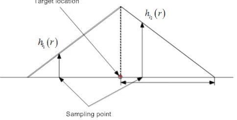
When the target dose not release the decoy, there is only one target in the radar beam and mk = 1. Setting the radar waveform to a rectangular pulse with a width of τ, the output of match filter is a triangular envelop with a width of 2τ. Assuming that the sampling rate of match filter is 1/τ, there are 2 sampling points (l1 and l2) affected by the target, where l1, l2 ∈ {1, . . . , L} and L are the sampling points for interest. The sampling model is shown in Figure 2, and hl1(r) = 1−mod(r,ΔR)/ΔR, hl2(r) = mod(r,ΔR)/ΔR represent the contribution of target to the two sampling points respectively,
where ΔR is the distance unit.
Figure 2. Sampling model with only one target in the radar beam.
The outputs of match filter of sum channel and azimuth channel in sampling points l1 and l2 are sI(l1) =α1cosφ+nsI(l1)
sI(l2) =α2cosφ+nsI(l2) sQ(l1) =α1sinφ+nsQ(l1) sQ(l2) =α2sinφ+nsQ(l2) dI(l1) =γα1cosφ+ndI(l1) dI(l2) =γα2cosφ+ndI(l2) dQ(l1) =γα1sinφ+ndQ(l1) dQ(l2) =γα2sinφ+ndQ(l2)
(4)
where αi (i = 1,2) is the amplitude of sampling point i, and γ is the monopulse ratio. They are correlated with radar pattern and target state through the following formula [51]:
αi= κ √
σhli(r)S2(θ)
r2 , γ =
D(θ)
S(θ), r =
x2+y2, θ= arctan(y/x)−θ
p (5)
whereκis a constant determined by the radar equation;σ is the RCS of target;θis the angle aviation of target; S(θ) and D(θ) are the antenna patterns of sum channel and difference channel, respectively; θp is the radar pointing. nsI(l),nsQ(l),ndI(l),ndQ(l) (l= 1, . . . , L) are the zero mean Gaussian noise with independent uniform distribution, and their variances are E[nsI(l)2] = E[nsQ(l)2] = σs2, E[ndI(l)2] =
E[ndQ(l)2] =σd2.
At this point, a single pulse signal vectorg composed of sum and difference channel signals is
The conditional distribution function ofg is
p(g|Xk, mk= 1) =N(g; 0,P) (7)
whereXk is the target state, and its model isXk= [x,x, y,˙ y˙]
P=
P1 0
0 P1
(8)
and
P1 = ⎡ ⎢ ⎣
α2
01 α01α02 α201γ α01α02γ α202 α01α02γ α202γ
α201γ α01α02γ2 α202γ
⎤ ⎥
⎦+ diag(σs2, σs2, σ2d, σ2d) (9)
whereα0i is the Rayleigh parameter related to αi.
2.2. Case 2: Observation Model with Unresolved Target and Decoy
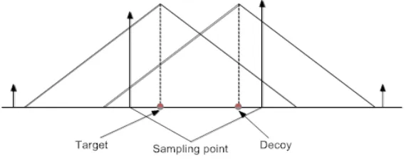
When the target releases the decoy, the number of targets increases to 2, and unresolved target and decoy are both within the same resolution cell. There are also two sampling points affected by the target and decoy, and the signals of these two sampling points are superimposed by the target and jamming signals. Their sampling model is shown in Figure 3.
Figure 3. Sampling model with target and decoy being in same resolution cell.
Similarly, the outputs of match filter of sum channel and azimuth channel in sampling points l1 and l2 are [50]
sI(l1) =α1,TcosφT +α1,DcosφD+nsI(l1) sI(l2) =α2,TcosφT +α2,DcosφD+nsI(l2) sQ(l1) =α1,TsinφT +α1,DsinφD+nsQ(l1) sQ(l2) =α2,TsinφT +α2,DsinφD+nsQ(l2)
dI(l1) =γTα1,TcosφT +γDα1,DcosφD +ndI(l1) dI(l2) =γTα2,TcosφT +γDα2,DcosφD +ndI(l2) dQ(l1) =γTα1,TsinφT +γDα1,DsinφD+ndQ(l1) dQ(l2) =γTα2,TsinφT +γDα2,DsinφD+ndQ(l2)
(10)
where αi,T (i= 1,2) is the amplitude of sampling pointi affected by target, andαi,D (i= 1,2) is the amplitude of sampling point iaffected by decoy.
The form of signal vectorg is
g = [sI(l1), sI(l2), dI(l1), dI(l2), sQ(l1), sQ(l2), dQ(l1), dQ(l2)]T (11)
When mk= 2, the conditional distribution function ofg is
In the same way
P=
P1 0
0 P1
(13)
where
P1 = ⎡ ⎢ ⎢ ⎣
α2
01,a α01,aα02,a α201,aγa α01,aα02,aγa
α202,a α01,aα02,aγa α202,aγa
α201,aγa α01,aα02,aγ2a
α2 02,aγa
⎤ ⎥ ⎥ ⎦
+ ⎡ ⎢ ⎢ ⎣
α201,b α01,bα02,b α012 ,bγb α01,bα02,bγb
α202,b α01,bα02,bγb α202,bγb
α201,bγb α01,bα02,bγb2
α202,bγb ⎤ ⎥ ⎥
⎦+ diag(σ2s, σs2, σd2, σ2d) (14)
3. JOINT DETECT AND TRACK WITH UNKNOWN NUMBER OF TARGETS
3.1. Joint Multi-Targets Probability Density Bayesian Filtering
The detection and tracking of unresolved target and decoy is essentially a joint detect and track for an unknown number of targets within the radar beam. Since the number of targets (include the target and decoy) within the radar beam is unknown and varying, a probability density model can describe the number of targets and targets state [52]. The joint multi-targets probability density
p(x1,k,x2,k, . . . ,xm,k, mk|Zk) is adopted to describe the conditional probability density of mk targets with their states x1,k,x2,k, . . . ,xm,k and the observation set Zk(Zk ={z1,z2, . . . ,zk}), which can be abbreviated asp(Xk, mk|Zk). p(∅, m= 0|Z) represents the posterior probability density when there is no target in the radar beam; p(xT, m= 1|Z) represents the posterior probability density when only one target is in the radar beam; and p(xT,xD, m= 2|Z) represents the posterior probability density when both the target and decoy are in the radar beam.
The dimension of state vector Xk is determined by the number of targets in the beam at time k; therefore, this problem can be transformed into a mixed estimation problem of the number and state of targets. The probability that there aremtargets in radar beam is obtained by the integration of the joint multi-targets probability density.
⎧ ⎪ ⎨ ⎪ ⎩
p(m|Z) = p(x1, . . . ,xm, m|Z)dx1. . . dxm ∞
m=0
p(m|Z) = 1 (15)
According to the Chapman-Kolmogorov equation, the state prediction equation is
p(Xk, mk|Zk−1) =
∞
mk−1=0
p(Xk, mk|Xk−1, mk−1)p(Xk−1, mk−1|Zk−1)dXk−1 (16)
wherep(Xk, mk|Xk−1, mk−1) is the Markov state transfer function. Using the Bayesian criterion, the updated equation for the state is
p(Xk, mk|Zk) = p
(zk|Xk, mk)p(Xk, mk|Zk−1) p(zk|Zk−1)
(17)
It is easy to estimate the number of targets mk and their stateXkaccording top(Xk, mk|Zk), and thus the detection of target or decoy and the tracking of unresolved targets within the radar beam are able to be realized simultaneously.
distribution of the signal vector composed by M pulses G={gm}Mm=1 (where gm is the signal vector of mth pulse) is
p(G|Xk, mk) = M
m=1
p(gm|Xk, mk) (18)
Define the observation vector of the mth pulse as zm = [zmI,zmQ]T, where I means in-phase component, andQmeans quadrature component.
zmI = [sI(1), . . . , sI(L), dI(1), . . . , dI(L)]T
zmQ = [sQ(1), . . . , sQ(L), dQ(1), . . . , dQ(L)]T
(19)
The observation vectors of M pulses constitute a complete measurement of radar at time k:
zk={zm}Mm=1 (20)
If there is no target in the radar beam, the signals of sampling point are background noise, then the likelihood function of single sampling pointl is
p(zm(l)|mk = 0) =N(zm(l); 0,P) (21) whereP = diag(σs2, σd2, σ2s, σd2).
Therefore, the observation likelihood function under the condition of the target number mk and target states Xk can be obtained as
p(zk|Xk, mk) = ⎧ ⎪ ⎪ ⎪ ⎪ ⎪ ⎪ ⎪ ⎪ ⎪ ⎪ ⎨ ⎪ ⎪ ⎪ ⎪ ⎪ ⎪ ⎪ ⎪ ⎪ ⎪ ⎩
M
m=1
L
l=1
N(zm(l); 0,P) if mk= 0
M
m=1
L
l=1
N(zm(l); 0,P) M
m=1
p(gm|Xk, mk)
M
m=1
L
l∈S
N(zm(l); 0,P)
if mk= 1,2
(22)
whereS is the sample point set related to target stateXk.
3.2. Joint Detection and Tracking Based on Particle Filter
The joint multi-targets probability density Bayesian filtering involves integral operations, and direct calculation has high implementation complexity. The sequential importance-resampling particle filtering method can achieve approximate calculation. Utilize N particles {Xk(n), mk(n), w(kn)}Nn=1 to approximate the joint multi-targets conditional probability density functionp(Xk, mk|Zk), and realize the estimation for the target numbermkand corresponding target state vector Xk, wherem(kn)is the number of targets fornth particle, and corresponding to differentm(kn), there are [53]:
Whenm(kn) = 0,Xk(n)=∅, there is no target in the radar beam;
Whenm(kn) =1, Xk(n)={x(k,Tn)}, there is only target in the radar beam;
When m(kn) =2, Xk(n) = {x(k,Tn),x(k,Dn)}, there are target and decoy in the radar beam. T denotes target, and Ddenotes decoy.
The joint detection and tracking algorithm for unknown number of targets based on particle filter is implemented as follows.
3.2.1. Step 1: Initialization
Assume that the target, decoy and target number of initial density p(x0,T), p(x0,D) and
p(m0) 2
x0(n,D) (if exist) in order. The initialization method of m0(n) is: obtain un ∼ U[0,1] through sampling,
then m(0n) set as m ∈ M according
m−1
i=0
< un ≤ m i=0
μi. The initializations of states x(0n,T) and x
(n) 0,D
are the uniform distribution within the radar observation area. If m(0n) > 0 for the nth particle, the state vector of the target and the decoy for this particle are expressed as x(0n,T) = [x(0n,T),x˙
(n) 0,T, y
(n) 0,T,y˙
(n) 0,T]
and x(0n,D) = [x(0n,D),x˙
(n) 0,D, y
(n) 0,D,y˙
(n)
0,D], and they correspond to the distance and velocity in the X and
Y directions, respectively. The above components in the vectors are initialized by the radial range, velocity and angle of the monopulse radar. Assume that the initial antenna pointing of monopulse radar isp0= [r0p, θp0]T, wherer0p is the center of range gate of radar,θp0 the pointing of radar beam, and
BW the half power beamwidth of radar. Therefore, the position component of x(0n,T) and x
(n)
0,D can be obtained through the projection transformation in Cartesian coordinate system.
x(0n,T), y
(n) 0,T
T =r0(n,T)
cos
θ(0n,T)
,sin
θ0(n,T) T
x(0n,D), y
(n) 0,D
T
=r0(n,D)
cos
θ0(n,D)
,sin
θ(0n,D)
T (23)
where r0(n,T) and r0(n,D) are the initial radial ranges of target and decoy, and they follow the uniform
distribution in the range gate. θ0(n,T) and θ
(n)
0,D are the initial angle errors of target and decoy, and they also follow the uniform distribution in the beamwidth. The four components mentioned above can be obtained as
r0(n,T), r
(n) 0,D ∼U
r0p−ΔR·L/2, rp0+ ΔR·L/2
θ(0n,T), θ
(n) 0,D∼U
θ0p−BW/2, θp0+BW/2
(24)
Set the speed range [vmin, vmax] according to the target type and motion characteristics, and the velocity component of x(0n,T) and x(0n,D) can be obtained through the velocity projection as follows.
˙
x(0n,T),y˙
(n) 0,T
T =v0(n,T)
cos
θ(v,n0),T
,sin
θ(v,n0),T T
˙
x(0n,D),y˙
(n) 0,D
T
=v0(n,D)
cos
θv,(n0),D
,sin
θ(v,n0),D
T (25)
where v(0n,T) and v0(n,D) are the initial radial velocity of target and decoy, and they follow the uniform distribution in the speed range.
v(0n,T)v
(n)
0,D∼U[vmin, vmax] (26)
θ(v,n0),T and θv,(n0),D are the initial deviation angle of velocity, and they follow the uniform distribution in [0,2π].
θ(v,n0),T, θ
(n)
v,0,D ∼U[0,2π] (27)
3.2.2. Step 2: Prediction
This step is to predict the number of targets {m(kn|k)−1}Nn=1 and their state x (n)
k|k−1,T and/or x
(n)
k|k−1,D based on the value at the timek−1. With the number of targets {mk(n−)1}Nn=1 at time k−1 and their
transformation matrix in Eq. (2), {mk(n|k)−1}Nn=1, x (n)
k|k−1,T and/or x
(n)
k|k−1,D can be predicted by the following method:
(i) Generate the random value of target numberci(j) from the transformation matrix
(ii) By comparison, predict the target number for every particle: for particle n= 1 :N, generate the random numberuN ∼ U[0,1], simultaneously set i=mk(n−)1. Initial setting m = 1, if ci(m) < un, then m = m+ 1. Loop for every particle until n = N. Output the predicted target number {m(kn|k)−1}Nn=1 for every particle;
(iii) For particle n= 1 :N, if the predicted target numberm(kn|k)−1 > m(kn−)1, declare the newborn of the target or jamming, and newborn of target state is consistent with the initialization stage in Step 1;
(iv) Ifm(kn|k)−1 < m(kn−)1, declare the death of target, and the corresponding target state will be abandoned;
(v) For survival target, the state x(kn|k)−1,T and/or x(kn|k)−1,D are predicted by the state transformation densityfk|k−1(x|x) in (3).
3.2.3. Step 3: Update
The sampling importance resampling (SIR) is used to resample the particles. The likelihood ratio is used as the normalized weight.
˜
w(kn)=l(kn) p
zk|Xk(n|k)−1, m(kn|k)−1
p
zk|Xk(n|k)−1=∅, m(kn|k)−1= 0
(28)
Bring the observation likelihood of Eq. (22) into Eq. (28) will reduce the calculation quantity of likelihood function.
˜
w(kn)= p(zk|X (n)
k|k−1, m (n)
k|k−1) p(zk|Xk|k−1, mk|k−1 = 0)
= ⎧ ⎪ ⎪ ⎪ ⎪ ⎪ ⎪ ⎪ ⎪ ⎨ ⎪ ⎪ ⎪ ⎪ ⎪ ⎪ ⎪ ⎪ ⎩
1 if m(kn|k)−1= 0
M
m=1
p(gm|Xk(n|k)−1, m(kn|k)−1)
M
m=1
L
l∈S
N(zm(l); 0,P)
if m(kn|k)−1= 1,2 (29)
After obtaining the weight of all particles, normalize the weightwk(n|k)−1= ˜wk(n|k)−1/Nn=1w˜ (n)
k|k−1 and get weight {w(kn|k)−1}Nn=1.
3.2.4. Step 4: Resampling
In resampling step, the predicted termXk(n|k)−1andmk(n|k)−1, and the likelihood ratioslk(n)were all retained in the process. By this way, the relationship among these three vectors can be preserved without recomputation and thus save computation.
3.2.5. Step 5: MCMC Move
In order to reduce the degradation of particles, the MCMC move is introduced on the basis of resampling to increase the diversity of particles without changing their original distribution [54]. The Metropolis-Hasting resampling-moving method is used to reduce the degradation in the target error angle estimation: for the particles satisfying m(kn) > 0, select an appropriate recommended distributionqm(θk|θk) =N(θk;θk, σm2), and then obtain the new state θk,T and θk,D through sampling this distribution. Replace the position component of the target and decoy in particle Xkn through Eq. (30) to get a new particle Xk(n).
xk,T(n), yk,T(n)
=
cosθk,T x(k,Tn),sinθk,T yk,T(n)
T
xk,D(n), yk,D(n)
=
cosθk,D x(k,Dn),sinθk,D yk,D(n)
Calculate the likelihood ratio corresponding to following formula and determine whether to accept the new particle or not.
Tmove =
p
zk|Xk(n)
p
zk|Xk(n)
= l
(n)
k
lk(n)
(31)
IfTmove>1, the new particle X
(n)
k will be reserved and replace old particlesX
(n)
k ; otherwise only when U < Tmove, the new particles will be reserved, whereU is one sampling of distribution U(0,1).
3.2.6. Step 6: Detection and State Estimation
The particles before resampling are used to estimate the state of target and decoy. The estimation of target numbermk is
ˆ
mk= N
n=1
w(kn|k)−1m(kn|k)−1 (32)
After ˆmk is obtained, the detection of target and decoy is decided as ⎧
⎨ ⎩
ˆ
mk < T1 ⇒no target T1<mˆk≤T2 ⇒only target
ˆ
mk > T2 ⇒target and decoy
(33)
whereT1 ∈0,1 andT2∈1,2 are two detection thresholds of this hypothesis testing problem. The state estimation of target is obtained as
ˆ xk,T =
n∈N1
w(kn|k)−1x(kn|k)−1,T
n∈N1
wk(n|k)−1 (34)
The state estimation of decoy is obtained as
ˆ xk,D =
n∈N2
w(kn|k)−1x(n)
k|k−1,D
n∈N2 wk(n|k)−1
(35)
whereN1, N2 are the particle set that satisfies mk(n|k)−1 >0.
After above recursive filtering, the detection of target and decoy can be realized timely and accurately, and the state of target and decoy can be estimated correctly after the jamming is detected.
4. SIMULATION AND EXPERIMENT
4.1. Simulation Setting
(a) Trajectory of target and decoy
(b) Range difference (c) Angle error
r
−
r (m)
12
Y (m)
3.2 3.3 3.4 3.5 3.6 3.7 3.8 3.9 4
X (m) 4
3.9
3.7
3.5
3.4
3.2 3.8
3.6
3.3
0 5 10 15 20 25 30 35 40
Time(s) 40
35
25
15
10
0 30
20
5
45 50
DOA (deg)
0.7
0.6
0.4
0.2
0.1 0.5
0.3
0
0 5 10 15 20 25 30 35 40
Time(s)
45 50 Target
Decoy Target
Decoy
Figure 4. Scene setting of simulation.
Mk
5 10 15 20 25 30 35 40 45 50 55 60
Time(s)
2.5
2
1.5
1
0.5
0
estimate truth
Figure 5. The estimation result of target numbers in radar beam when ISR= 2.
y (km)
32 33 34 35 36 37 38 39 40
x (km)
40
39
37
35
34
32 38
36
33
estimate truth
In the experiment, the radar adopts the monopulse model, and the half power beamwidth of radar sum channelBW = 2.4◦. The noise variance of real and imaginary components of sum channel is set to
σ2
s =σd2 = 1, and the SNR of single pulse is defined as
SNR = E(α 2
i)
σ2
s
= E(α 2 i) σ2 d = σκ¯ 2
r4 (36)
where assumehli(r) = 1 andF2 (θ) = 1. The signal power of target and decoy is decided by the average radar cross section (ARCS) ¯σ, and the interference suppression ratio is equal to ¯σT/σ¯D, whereT denote the target and D the decoy. The radar constant κ is equal to the square of the initial range of target:
κ =r2
0,T. Therefore, the SNR is only controlled by the ARCS and the range of the target and decoy. In this scenario, the range between radar and target is approaching gradually, and the SNR increases gradually. The dwell time interval in radar beam is T = 1 s, the number of pulses M = 40, and the range unit ΔR= 45 m.
The motions of target and decoy are approximated as a constant velocity model, where the state transformation matrix and noise covariance are shown as follows.
F= ⎡ ⎢ ⎣
1 T 0 0
0 1 0 0
0 0 1 T
0 0 0 1
⎤ ⎥
⎦, Q=σw2
⎡ ⎢ ⎢ ⎢ ⎢ ⎢ ⎢ ⎢ ⎢ ⎢ ⎢ ⎢ ⎣ T4 4 T3
2 0 0
T3
2 T
2 0 0
0 0 T
4
4
T3
2
0 0 T
3 2 T 2 ⎤ ⎥ ⎥ ⎥ ⎥ ⎥ ⎥ ⎥ ⎥ ⎥ ⎥ ⎥ ⎦ (37)
The initial distribution of m0 is set as μ0= 0.8,μ1 = 0.1 and μ2 = 0.1, and the transfer matrix of mk is set as
Π =
0.8 0.1 0.1 0.1 0.8 0.1 0.1 0.1 0.8
(38)
5. SIMULATION RESULTS
Experiment 1: In the implement of MALD jamming, in order to attract and deceive the radar beamforming to point to the false angle of jamming, usually the power of decoy is greater than that of target echo, and the typical interference suppression ratio is ISR= 2∼8. The joint detection and tracking results with the jamming scene ofISR= 2 are shown in the following figures. 200 times Monte Carlo simulation are utilized to evaluate the performance of the algorithm. The initial SNR is 0 dB, and the detection threshold is set as T1= 0.5 and T2 = 1.5.
Figure 5 shows the mean of estimated number of targets in the radar beam. The number of targets exceeds the threshold T1 at the 12th time step, and this indicates that the target is detected. The reality is that the target appears at the 11th time step, so the detection delay is about one time step. The number of targets exceeds the thresholdT2 at the 32th time step, and this indicates that the decoy is released by the target, and the detection delay is about 2 time step compared to the actual decoy releasing time.
Time(s)
10 15 20 25 30 35 40 45 50 55 60
Range RMSE (m)
0 100 200 300 400 500 600 700 800 900 1000
Target Decoy
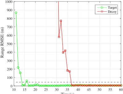
Figure 7. RMSE of range estimation when
ISR= 2.
Time(s)
10 15 20 25 30 35 40 45 50 55 60
Angle RMSE (deg)
0 0.1 0.2 0.3 0.4 0.5 0.6 0.7 0.8 0.9
Target Decoy
Figure 8. RMSE of angle estimation when
ISR= 2.
Time(s)
10 15 20 25 30 35 40 45 50 55 60
Position RMSE (m)
0 500 1000 1500 2000 2500 3000
Target Decoy
Figure 9. RMSE of position estimation when
ISR= 2.
Mk
5 10 15 20 25 30 35 40 45 50 55 60 Time(s)
2.5
2
1.5
1
0.5
0
Figure 10. Estimation results of target number under different ISR.
The simulation results of above experiment show that the proposed joint detection and tracking algorithm of unresolved target and decoy is available to detect the occurrence of MALD jamming, and the detection delay is no more than 5 time steps. The accurate estimation of target and decoy states can be achieved, and the estimation error is small. This ability can meet the needs of stable tracking.
Experiment 2: Based on experiment 1, the performance of joint detection and tracking algorithm for unresolved multi-targets under different ISR conditions is investigated to verify the adaptability of the algorithm to different jamming conditions. Six typical jamming conditions are selected, and 200 times Monte Carlo experiments are also used for performance evaluation. The results of target number estimation in radar beam under different ISR conditions are shown in the following figures.
It can be seen in Figure 10 that the detection delay of target is maintained at one time under different ISR conditions, and the detection of decoy releasing is continuously improved as the ISR increases. The larger the ISR is, the faster the estimated target number rises to 2 after the decoy releasing; therefore, the detection delay is smaller, and the detection performance is better.
The state estimation results of the target and decoy under different ISR conditions are shown in the figures.
(a) Tracking trajectory for all time
y (km)
32 33 34 35 36 37 38 39 40
x (km)
40
39
37
35
34
32 38
36
33
y (km)
32.5 33 33.5 34 34.5 35 35.5 36
x (km)
36
35.5
34.5
33
32.5 .35
33.5
32 34
(b) Detail feature of the tracking trajectory
Figure 11. Tracking trajectory of target and decoy under different ISR conditions.
(a) Target range estimation RMSE (b) Decoy range estimation RMSE
Range RMSE (m)
Time(s)
30 35 40 45 50 55 60
Position RMSE (m)
0 500 1000 1500 2000 2500
3000 Decoy Position Estimation RMSE
ISR=1 ISR=3 ISR=5 ISR=7 Target Range Estimation RMSE
2500
2000
1500
1000
500
0
10 15 20 25 30 35 40 45 50 55 60
Time(s)
Figure 12. Range estimation RMSE of proposed algorithm under different ISR conditions.
(a) Target angle estimation RMSE
Angle RMSE (deg)
(b) Target angle estimation RMSE
Decoy Position Estimation RMSE Target Range Estimation RMSE
0.7
0.6
0.4
0.2
0.1 0.5
0.3
0
10 15 20 25 30 35 40 45 50 55 60
Time(s)
Angle RMSE (deg)
0.9
0.8
0.4
0.2
0.1 0.5
0.3
0 0.7
0.6
Time(s)
30 35 40 45 50 55 60
(a) Target position estimation RMSE (b) Target position estimation RMSE
Decoy Position Estimation RMSE Target Range Estimation RMSE
Position RMSE (m)
2500
2000
1500
1000
500
0
10 15 20 25 30 35 40 45 50 55 60
Time(s) Time(s)
30 35 40 45 50 55 60
Position RMSE (m)
0 500 1000 1500 2000 2500 3000
Figure 14. Position estimation RMSE of proposed algorithm under different ISR conditions.
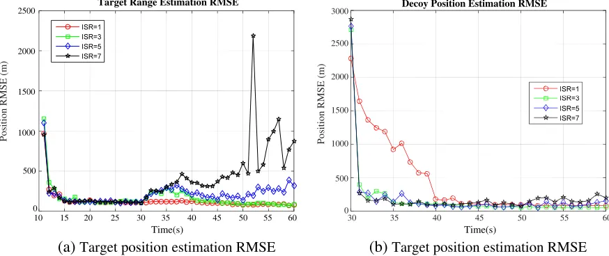
The range estimation RMSEs, angle estimation RMSEs, and position estimation RMSEs of target and decoy under different ISR conditions are shown in Figure 12, Figure 13, Figure 14, respectively.
It can be seen form above figures that the estimation errors of the decoy in the range, angle and position are all small, with the exception of at the beginning of the experiment when the decoy is just released. Different from the decoy, the estimation errors of the true target in range angle and position are related to the ISR conditions, and with the increase of the ISR, the estimation accuracy of target decreases a little. Especially in the condition of strong jamming of ISR= 7, the estimation accuracy of target becomes worse, and the estimation error increases. Overall, the proposed algorithm has a good performance in both detection correctness and estimation accuracy, and can ensure the monopulse radar to always detect and track the target and decoy stably before the target is deceived to exit from the radar beam.
6. CONCLUSIONS
In this study, the counteracting of typical MALD jamming of a monopulse radar was investigated. Through the establishment of measurement model of target and decoy, a joint detection and tracking algorithm of unresolved target and decoy that utilized multi-targets probability density was developed. Simulation results showed that the proposed algorithm was capable of quickly and accurately detecting the existence of the true target and the decoy, and estimating the position of both. The estimation error was observed to be small, and this ensured that the monopulse radar detected and tracked the target stably before the target was deceived to escape form the radar beam.
ACKNOWLEDGMENT
This work was supported in part by the National Natural Science Foundation of China (No. 61401475).
REFERENCES
1. Knowles, J., “MALD-J passes design milestone,”The Journal of Electronic Defense, Vol. 33, No. 2, 16–18, 2010.
2. Goodman, G., “MALD testing successful,” The Journal of Electronic Defense, Vol. 31, No. 4, 16–17, 2008.
4. Zhang, T., Z. Zhou, L. Yu, et al., “Coordinated evasion strategy for MALD and fighter in air combat,”System Engineering and Electronics, Vol. 39, No. 12, 2739–2744, 2017.
5. Mao, Y., Y. Han, Q. Guo, and G. Yu, “Simulation and analysis of MALD blanket jamming,” Modern Radar, Vol. 36, No. 1, 11–14, 2014.
6. Dai, H., H. Han, J. Wang, X. Xu, and H. Qiao, “An improved high angular resolution method by using four-channel jointed monopulse radar,” 2017 Progress In Electromagnetics Research
Symposium — Spring (PIERS), 3056–3061, St Petersburg, Russia, May 22–25, 2017.
7. Wu, J., Z. Xu, Z. Xiong, et al., “Resolution of multiple unresolved targets via dual monopulse with array radar,”Proceeding of 2014 11th European Radar Conference, 1–4, Rome, Italy, 2014.
8. Lu, D. and Y. Li, “Study on resolution limit of space-time 2D joint processing,” Transactions of Beijing Institute of Technology, Vol. 33, No. 2, 203–207, 2013.
9. Wang, L., Z. Xu, X. Liu, et al., “Estimation of unresolved targets number based on Gerschgorin disks,”Proceeding of 2017 IEEE International Conference on Signal Processing, Communications and Computing (ICSPCC), 1–5, Beijing, China, 2017.
10. Bosse, J. and O. Rabaste, “Subspace rejection for matching pursuit in the presence of unresolved targets,”IEEE Transactions on Signal Processing, Vol. 66, No. 8, 1997–2010, 2018.
11. Lu, Z., F. Li, and T. Zeng, “Monopulse radar angle extractor of multiple unresolved targets via matching pursuits,”Proceeding of IET International Radar Conference, 1–5, Xian, China, 2013. 12. Li, Y., T. Zeng, B. Ji, et al., “Angle-tracking for two unresolved targets by high resolution
spectrum analysis and pipeline technique,” Proceeding of 2006 8th international Conference on Signal Processing, 11–14, Guilin, China, 2006.
13. Gorji, A. A., R. Tharmarasa, W. D. Blair, et al., “Multiple unresolved target localization and tracking using colocated MIMO radars,”IEEE Transactions on Aerospace and Electronic Systems, Vol. 48, No. 3, 2498–2517, 2012.
14. Glass, J. D. and L. D. Smith, “Unresolved measurement processing with widely separated radars using sparse modeling,” Proceeding of 2012 IEEE Radar Conference, 940–945, Atlanta, Georgia, USA, 2012.
15. Ma, J., L. Shi, J. Liu, et al., “Improved two-targets resolution using dual-polarization radar with interlaced subarray partition,” Proceeding of 2017 13th IEEE International Conference on Electronic Measurement & Instruments (ICEMI), 397–400, Qingdao, China, 2017.
16. Zhao, Y. N., Z. Q. Zhou, and X. L. Qiao, “Angle estimation for two closely spaced targets with polarization monopulse radar,” Proceeding of 2005 Asia-Pacific Microwave Conference, 3– 8, Suzhou, China, 2005.
17. Blair, W. D. and M. Brandt-Pearce, “Unresolved Rayleigh target detection using monopulse measurements,” IEEE Transactions on Aerospace and Electronic Systems, Vol. 34, No. 2, 543– 552, 1998.
18. Glass, J. D. and W. D. Blair, “Detection of unresolved Rayleigh targets using adjacent bins,” Proceeding of 2016 IEEE Aerospace Conference, 1–7, Big Sky, Montana, 2016.
19. Zhao, F., J. Yang, M. Dan, et al., “Detection of presence of multiple unresolved targets based on range glint,” ACTA Electronica Sinica, Vol. 36, No. 12, 2290–2298, 2008.
20. Zhao, F., L. Bi, and T. Min, “A new method for detecting the presence of multiple unresolved targets,”ACTA Electronica Sinica, Vol. 38, No. 10, 2258–2263, 2010.
21. Blair, W. D. and M. Brandt-Pearce, “Monopulse DOA estimation of two unresolved Rayleigh targets,”IEEE Transactions on Aerospace and Electronic Systems, Vol. 37, No. 2, 452–469, 2001. 22. Lee, S.-P., B.-L. Cho, S.-M. Lee, et al., “Unambiguous angle estimation of unresolved targets
in monopulse radar,” IEEE Transactions on Aerospace and Electronic Systems, Vol. 51, No. 2, 1170–1177, 2015.
23. Li, H., J. Deng, and X. Wang, “Monopulse DOA estimation of two unresolved targets with SNR estimation,” Proceeding of 2015 IEEE Advanced Information Technology, Electronic and
24. Sinha, A., T. Kirubarajan, and Y. Bar-Shalom, “Tracker and signal processing for the benchmark problem with unresolvedtargets,”IEEE Transactions on Aerospace and Electronic Systems, Vol. 42, No. 1, 279–300, 2006.
25. Zhang, X., P. K. Willett, and Y. Bar-Shalom, “Monopulse Radar detection and localization of multiple unresolved targets via joint bin processing,” IEEE Transactions on Signal Processing, Vol. 56, No. 3, 1302–1308, 2005.
26. Wang, Z., A. Sinha, P. Willett, et al., “Angle estimation for two unresolved targets with monopulse radar,”IEEE Transactions on Aerospace and Electronic Systems, Vol. 40, No. 3, 998–1019, 2004. 27. Ehrman, L. M. and W. D. Blair, “Accounting for frequency dilation of the monopulse ratio
when using the joint multiple bin processing,” Proceeding of 2006 Proceeding of the Thirty-Eighth
Southeastern Symposium on System Theory, 230–234, Cookeville, TN, USA, 2006.
28. Jeong, S. and J. K. Tugnait, “Tracking of two targets in clutter with possibly unresolved measurements,” IEEE Transactions on Aerospace and Electronic Systems, Vol. 44, No. 2, 748– 765, 2008.
29. Svensson, D., M. Ulmke, and L. Danielsson, “Joint probabilistic data association filter for partially unresolvedtarget groups,”Proceeding of 13th International Conference on Information Fusion, 1–8, Edinburgh, UK, 2010.
30. Henk, A., P. Blom, and E. A. Bloem, “Bayesian tracking of two possibly unresolved maneuvering targets,”IEEE Transactions on Aerospace and Electronic Systems, Vol. 43, No. 2, 612–627, 2007. 31. Davey, S. J., “Tracking possibly unresolved targets with PMHT,” Proceeding of IEEE 2007
Information, Decision and Control, 47–52, Adelaide, Australia, 2007.
32. Mahler, R., Statistical Multisource Multitarget Information Fusion, Artech House, Norwood, MA, 2007.
33. Mahler, R., Advances in Statistical Multisource-Multitarget Information Fusion, Artech House, Norwood, MA, 2014.
34. Mahler, R., “PHD filters for nonstandard targets, II: Unresolved targets,” Proceeding of 2009 12th International Conference on Information Fusion, 922–929, Seattle, Washington, USA, 2009. 35. Erdinc, O., P. Willett, and Y. Bar-Shalom, “Probability hypothesis density filter for multitarget
multisensor tracking,” Proceeding of 2005 7th International Conference on Information Fusion, 8–15, Philadelphia, PA, USA, 2005.
36. Beard, M., B.-T. Vo, and B.-N. Vo, “Bayesian multi-target tracking with merged measurements using labelled random finite sets,” IEEE Transactions on Signal Processing, Vol. 63, No. 6, 1433– 1447, 2015.
37. Li, Y., H. Xiao, and H. Wu, “Joint tracking and identification of the unresolved towed decoy and aircraft using the labeled particle probability hypothesis density filter,” Proceeding of 2015 8th International Congress on Image and Signal Processing (CISP), 1442–1447, Shenyang, China, 2015.
38. Lian, F., Y. Xiang, and H. Chen, “Tracking unresolved targets using cardinalized probility hypothesis density filter,” System Engineering and Electronics, Vol. 35, No. 12, 2445–2451, 2013. 39. Zhang, G., F. Lian, and C. Han, “CBMeMBer filters for nonstandard targets, II: Unresolved
targets,” Proceeding of 17th International Conference on Information Fusion (FUSION), 1–6, Salamanca, Spain, 2014.
40. Yan, B., L. Xu, M. Q. Li, et al., “Track-before-detect algorithm based on dynamic programming for multi-extended-targets detection,” IET Signal Processing, Vol. 11, No. 6, 674–686, 2017. 41. Chen, H., P. Krishna, T. Kirubarajan, et al., “General data association with possibly unresolved
measurements using linear programming,”Proceeding of 2003 Conference on Computer Vision and
Pattern Recognition Workshop, 103–108, Portland, OR, USA, 2003.
42. Xiong, Y. and X. Wang, “A TBD algorithm to detect slow dim target based on Hough transform,”
6th International Conference on Wireless, Mobile and Multi-Media (ICWMMN 2015), 313–317,
43. Yu, H., G. Wang, Q. Cao, et al., “A fusion based particle filter TBD algorithm for dim targets,” Chinese Journal of Electronics, Vol. 24, No. 3, 590–595, 2015.
44. Isaac, A., X. Zhang, P. Willett, et al., “A particle filter for tracking two closely spaced objects using monopulse radar channel signals,”IEEE Signal Processing Letters, Vol. 13, No. 6, 357–360, 2006.
45. Isaac, A., P. Willett, Y. Bar-Shalom, “MCMC methods for tracking two closely spaced targets using monopulse radar channel signals,” IET Radar, Sonar & Navigation, Vol. 1, No. 3, 221–229, 2007.
46. Isaac, A., P. Willett, and Y. Bar-Shalom, “Quickest detection and tracking of spawning targets using monopulse radar channel signals,” IEEE Transactions on Signal Processing, Vol. 56, No. 3, 1302–1308, 2008.
47. Nandakumaran, N., A. Sinha, T. Kirubarajan, “Joint detection and tracking of unresolved targets with monopulse radar,” IEEE Transactions on Aerospace and Electronic Systems, Vol. 44, No. 4, 1326–1341, 2008.
48. Song, Z., H. Xiao, Y.-L. Zhu, et al., “A novel approach to detect the unresolved towed decoy in terminal guidance,”Chinese Journal of Electronics, Vol. 21, No. 2, 367–373, 2012.
49. Li, X. R. and V. Jilkov, “Survey of maneuvering target tracking: Part I. Dynamic models,” IEEE Transactions on Aerospace and Electronic Systems, Vol. 39, No. 4, 1333–1364, 2003.
50. Zhang, X., P.-K. Willet, and Y. Bar-Shalom, “Monopulse radar detection and localization of multiple unresolved targets via joint bin processing,” IEEE Transactions on Signal Processing, Vol. 53, No. 4, 1225–1236, 2005.
51. Skolnik, M. I., Introduction to Radar Systems, 3rd Edition, McGraw-Hill, New York, 2001.
52. Kreucher, C., K. Kastella, and A. O. I. Hero, “Multitarget tracking using the joint multitarget probability density,” IEEE Transactions on Aerospace and Electronic Systems, Vol. 41, No. 4, 1396–1414, 2005.
53. Cai, F., “Research on detection and tracking technologies for dim targets in radar,” National University of Defense Technology, China, 2015.