Non-Iterative Eigenfunction-Based Inversion (NIEI) Algorithm
for 2D Helmholtz Equation
Nasim Abdollahi*, Ian Jeffrey, and Joe LoVetri
Abstract—A non-iterative inverse-source solver is introduced for the 2D Helmholtz boundary value problem (BVP). Microwave imaging within a chamber having electrically conducting walls is formulated as a time-harmonic 2D electromagnetic field problem that can be modelled by such a BVP. The novel inverse-source solver, which solves for contrast sources, is the first step in a two-stage process that recovers the complex permittivity of an object of interest in the second step. The unknown contrast sources, as well as the (permittivity) contrast, are represented using the eigenfunction basis associated with the chamber’s shape; canonical shapes allowing for analytically defined eigenfunctions. This whole-domain eigenfunction basis allows the imposition of constraints on the contrast-source expansion at virtual spatial points or contours outside the imaging domain. These constraints effectively regularize the inverse-source problem and the result is a well-conditioned matrix equation for the contrast-source coefficients that is solved in a least-squares sense. The contrast-source coefficients corresponding to different illuminating fields are then utilized to recover the contrast expansion coefficients using one more well-conditioned matrix inversion. The performance of this algorithm is studied using a series of synthetic test problems. The results of this study are promising as they compare very well with, and at times out-perform, state-of-the-art inversion algorithms (both in terms of reconstruction quality and computation time).
1. INTRODUCTION
Microwave Imaging (MWI) can be a powerful diagnostic tool in a wide range of applications such as structural health monitoring [1], through-wall imaging [2], remote sensing [3, 4], and biomedical imaging [5–7]. The latter is of interest herein because in many cases the imaging can be performed within an imaging chamber, e.g., breast imaging, and the algorithm we describe is applicable to solving the inverse problem governed by a Helmholtz boundary value problem (BVP). Performing MWI within a conducting chamber can lead to various advantages as described in [8–10]. Although this algorithm is applicable to any Helmholtz BVP, we demonstrate it for the 2D Transverse-Magnetic (TM) formulation of MWI.
Quantitative MWI typically consists of minimizing a cost functional that is nonlinear and ill-posed [11, 12]. The nonlinearity is typically addressed utilizing local optimization techniques such as the Gauss-Newton [13, 14], the Conjugate gradient [15, 16], the Quasi-Newton [17], and the modified gradient [18] techniques, or even global optimization methods [19]. These are computationally intensive iterative procedures for minimizing a nonlinear cost-functional.
Developing robust computational techniques that deal with the ill-posedness remains a challenge [20]. The fundamental difficulty is related to the insufficient amount of information available to reconstruct the physical properties of interest with sufficient accuracy and resolution.
Received 26 March 2019, Accepted 26 June 2019, Scheduled 12 July 2019
* Corresponding author: Nasim Abdollahi ([email protected]).
Regularization methods implicitly or explicitly add information to help mitigate the ill-posedness. Tikhonov regularization is probably the most well-known regularization method [21] but several others have been developed such as those based on Singular Value Decomposition (SVD): Truncated SVD (TSVD) [22, 23], Generalized SVD (GSVD) [24], and the Modified Truncated SVD (MTSVD) [25]. The L-curve technique tries to balance the additional information added to the data-error functional when using Tikhonov regularization [26, 27]. All of these can lead to a well-posed problem with a stabilized good approximate solution of the original ill-posed problem [11, 28].
The non-iterative inversion algorithm described herein addresses the nonlinearity and ill-posedness of the inverse problem by means of a formulation that utilizes, as basis functions, the (whole-domain) eigenfunctions associated with the Helmholtz BVP with homogeneous Dirichlet boundary conditions. This results in one-to-one correspondence between the contrast source and scattered field expansion coefficients. A novel regularization approach that imposes the constraint that the contrast source is zero outside the imaging domain is also introduced. Such a constraint is possible because of the utilization of whole-domain basis functions whose support lies outside the imaging domain. We refer to this new technique as the Non-Iterative Eigenfunction-based Inversion (NIEI) algorithm.
Expanding the unknown contrast function using various types of basis for electromagnetic inverse problems was previously reported in the literature. For example, a modified gradient optimization in conjunction with the distorted Born iterative method has been used with regularization achieved by projecting the unknown contrast onto a finite wavelet basis [29, 30]. A patient-specific Gaussian function basis was introduced to reduce the number of unknowns and enable solving the 3D inverse scattering problem for breast imaging [31]. The efficiency of such projection methods and the accuracy of the solution is influenced by the choice and number of basis functions [30].
The use of eigenfunctions of the Helmholtz BVP has already been shown to provide promising results as reported in [8, 32]. In [8], the eigenfunction basis was discretized on a pixel-based mesh associated with the Contrast Source Inversion (CSI) formulation of a 2D TM inverse problem. In [32], instead of a grid-based discrete representation, the unknowns are projected on a whole-domain eigenfunctions basis, which is iteratively adapted during the optimization procedure. Both of these algorithms are iterative schemes. To the best of our knowledge the NIEI algorithm described herein is the first of its kind to achieve a robust direct non-iterative inversion.
The formulation of the NIEI algorithm for the inverse source problem is presented in Section 2. Two sets of constraints are proposed for regularization allowing the system matrix to be solved non-iteratively for a finite number of terms in the eigenfunction basis. In Section 3, the second stage of the algorithm that recovers the contrast profile is described. Then, in Section 4, an analysis of the NIEI algorithm for a single source inversion is provided. Available options for regularization are evaluated in Section 4.1. Next, in Section 5, we present the results of the contrast recovery stage for four numerical test cases. We quantify the resolution performance of the algorithm by conducting a suitably-designed test, similar to the test presented in [33], to illustrate the separation resolution limit of the system. Finally, the results and the algorithm’s performance are discussed in Section 6.
2. NON-ITERATIVE CONTRAST SOURCE RECOVERY
2.1. Problem Formulation
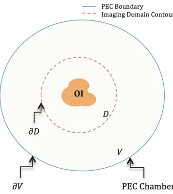
The first stage of the NIEI algorithm is the inverse-source solver for the Helmholtz BVP. As shown in Fig. 1 we consider an object-of-interest (OI) illuminated by a monochromatic point-source both located within a chamber having volume V and perfect electric conducting (PEC) boundary∂V. For each transmitting point-source the field is measured at discreet spatial locations outside the imaging domain,D, having boundary∂D. We assume a 2D TM-polarized problem with only theEzelectric-field component oriented along the axis of the chamber. The Ez field component, which we refer to as u, satisfies the Helmholtz BVP:
Δu(r) +k2(r)u(r) =−S(r); r∈V
u(r) = 0; r∈∂V (1)
where Δ represents the Laplacian operator; k is the wavenumber, defined as k2(r) = ω2
r(r)0μ0; 0
Figure 1. An example of a PEC-enclosed microwave imaging problem domains.
S(r). The final goal is to determine r(r), the complex-valued permittivity of the inhomogeneous OI, from the measurements. The OI is assumed to be non-magnetic.
The incident field, denoted asui, is the known field produced by sourceS(r) in the absence of the OI. The difference between the total field, u(r), and the incident field is defined as the scattered field,
us u−ui. Bothui andus satisfy inhomogeneous Helmholtz equations with different right-hand sides
but with the same constant background wavenumberk2b =ω2b0μ0, and Dirichlet boundary conditions:
Δui(r) +k2bui(r) =−S(r); r∈V
ui(r) = 0; r∈∂V (2)
and
Δus(r) +k2
bus(r) =−w(r); r∈V
us(r) = 0; r∈∂V (3)
Here b is the dielectric constant of the homogeneous background medium which is taken to be a uniform constant value throughout the imaging chamber. The right-hand side of the scattered field partial differential equation (PDE) is the contrast source,w(r), defined asw(r)kb2χ(r)u(r) where the contrast, χ(r), is defined asχ(r)(r(r)−b)/b.
2.2. Eigenfunction Basis
The associated set of eigenfunctions,{vn}, and eigenvalues, {μn}, for the problem satisfy:
Δvn(r) +kb2vn(r) =μnvn(r); r∈V
vn(r) = 0; r∈∂V (4)
These form a complete orthonormal basis which we use to expand all fields as well as the contrast and contrast-source variables:
⎧ ⎪ ⎪ ⎪ ⎪ ⎨ ⎪ ⎪ ⎪ ⎪ ⎩
u=
N
n γt
nvn, ui = N
n γi
nvn, us= N
n γs
nvn
w=
N
n γw
nvn, χ=
N
n γχ
nvn
(5)
(using inner product notation) as
ψ,ΔφV − φ,ΔψV ≡ ψ, ∂nφ∂V − φ, ∂nψ∂V (6) and applying it to the eigenfunctions vn and the scattered field us inside V, taking into account the boundary conditions given in Eqs. (3) and (4), we get
vn,ΔusV − us,ΔvnV = 0. (7)
Substituting for the Laplacian’s from the corresponding Helmholtz equations (3) and (4), gives
μnvn, usV +vn, wV = 0. (8)
Introducing the truncated expansions in Eq. (5) into Eq. (8) and using the orthonormal property of the eigenfunctions, we arrive at the desired fundamental relation
γw =−Mγs (9)
whereM is the diagonal matrix of eigenvalues, and the column vectors γw and γsstore the expansion coefficients. This represents a one-to-one relation between the contrast-source and scattered-field coefficients: if one has access to the coefficients of the scattered field one would automatically have the coefficients of the contrast sources. Via measurements, one typically only has the scattered field at a finite number of discrete spatial locations outside the imaging domain, making the problem ill-posed. None-the-less, as will now be shown, an efficient non-iterative contrast-source inverse solver can be formulated based on this relation.
2.3. Data-equations for the Inverse-Source Solver
Making use of our expansion, data equations can be written in terms of field measurements at locations,
rx:
N
n
γnsvn(rx) = us(rx); rx∈V (10)
N
n
γns∂ζvn(rx) = ∂ζus(rx); rx∈V. (11)
Here ∂ζ is derivative with respect to theζ direction. The latter equation is useful when measurements are made at the PEC boundary of the chamber. On ∂V the tangential electric field is identically zero but the normal derivative, setting ζ = n, is related to the tangential magnetic field at the boundary that is not zero and measurable [34]. That is, from Maxwell’s equation the magnetic-field components for the TM-mode are related to Ez as
∂yEz=−jωμHx
∂xEz =jωμHy (12)
so the normal derivative of the scattered electric-field can be found by measuring the tangential scattered magnetic-field:
∂nEz =jωμ(ˆnxHy−nˆyHx) =jωμHt. (13)
As outlined in [34], collecting the magnetic field at the PEC boundary provides several practical advantages, including a reduction in modeling error.
In matrix form, Eq. (11) can be written as
V∂γs=δ (14)
where V∂ is an R × N matrix with elements consisting of the value of the derivative of the N eigenfunctions at theR receiver locations,
V∂ij =∂nvj(rxi); rx∈∂V (15)
Using the fundamental relation in Eq. (9), Eq. (14) is written as
−V∂M−1γw =δ (16)
providing a linear equation between the contrast-source coefficients and the collected data. The ill-posedness of the linear inverse-source problem means that this matrix equation is ill-conditioned for a large number of unknowns, requiring a regularization scheme.
2.4. Novel Regularization Approach
We have found that conventional regularization techniques, like Tikhonov and SVD, are not effective in mitigating the ill-posedness of the inverse-source problem approximated by the truncated eigenfunction expansion. The truncation already limits the spectrum of the approximation to, possibly, the best that can be achieved, and increasing the truncation number,N, without introducing additional information deteriorates the condition of matrix equation (16). Truncating the eigenfunction expansion to a suitably lowN to obtain a well-conditioned matrix equation does not provide sufficient resolution. Applying SVD to (16) in an attempt to mitigate the ill-condition of the matrix and extend the number of eigenfunctions utilized is not effective. Truncating the eigenfunction representation already limits the spectrum being reconstructed and therefore the SVD technique cannot improve the solution.
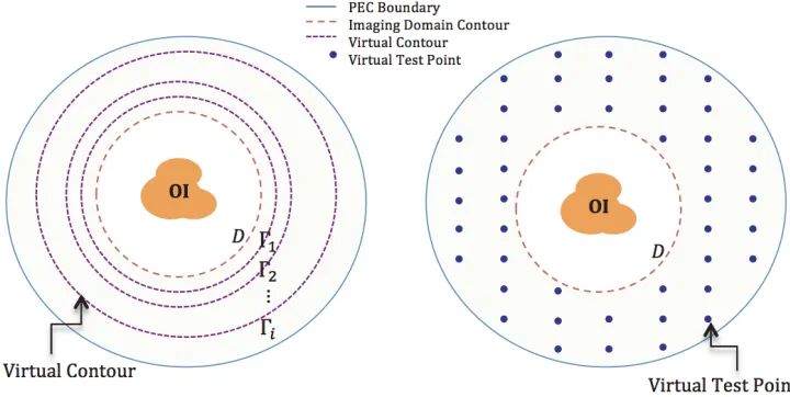
Fortunately, the use of whole-domain basis functions does allow us to introduce additional regularization that is based on incorporating prior knowledge that the contrast source is zero outside the imaging domain. This prior information has been imposed in two different ways; one we call virtual contours, and the other virtual test points (“virtual” because no real measurements are required).
Figure 2. An example of virtual constraints for regularization.
Virtual Contour Constraintsare derived by applying Green’s Theorem tovnandus in a region
V∗
i strictly outside the imaging domain bounded by Γi and ∂V as shown in Fig. 2. Thus, we have μnvn, usV∗
i +vn, wVi∗ =us, ∂nvnΓi − vn, ∂nusΓi, (17)
where∂n is the derivative with respect to the outward normal toVi∗ along Γi. Multiple subdomainsVi∗ can be chosen on which to enforce this constraint. The second term on the left-hand side of Eq. (17) is zero because the contrast source,w, is zero in Vi∗. Therefore, in matrix form, we have
(MKi−Di)γs =0, (18)
where theKmni element of the Ki matrix is defined as the inner product of two eigenfunctions over Vi∗:
Kimn =vn, vmV∗
i . (19)
The elements of theDi matrix are found as the line integrals
Di
Equation (18) can be applied to any arbitrary subdomain bounded by an arbitrary virtual contour Γi and ∂V, as long as contour Γi is inV∗ =V \D. Using the fundamental relation in Eq. (9), Eq. (18) can be written as
(MKi−Di)M−1γw =0, (21)
which represents a constraint on the eigenfunction expansion coefficients for the contrast source.
Virtual Test Point Constraintsare obtained by simply imposing that the contrast-source must be zero at a set of specified virtual test points, again within V∗. This is enforced directly via the contrast-source expansion (5):
N
n
γnwvn(rj) = 0; rj ∈V∗. (22)
In matrix form this becomes
Vγw =0, (23)
whereV is aJ ×N matrix of theN eigenfunctions evaluated atJ chosen test points.
The data and constraint Equations (16), (21), and (23) are solved simultaneously by concatenating the matrices and right-hand-sides into a final matrix equation of the formAγw =b:
⎡ ⎢ ⎢ ⎢ ⎢ ⎢ ⎢ ⎣
−V∂M−1
(MK1−D1)M−1
.. .
(MKI−DI)M−1 V ⎤ ⎥ ⎥ ⎥ ⎥ ⎥ ⎥ ⎦
γw=
⎡ ⎢ ⎢ ⎢ ⎣ δ 0 .. . 0 ⎤ ⎥ ⎥ ⎥ ⎦ (24)
whereI is the number of virtual contours at which the contour constraints are imposed.
Numerical studies show that with a sufficient number of constraints the eigenfunction-expansion truncation number, N, can be increased while retaining a well-conditioned matrix Equation (24). The problem is simply solved in the Least-Square sense:
γw = (ATA)−1ATb (25)
Note that the well-conditioned matrixAis independent of the incident field utilized to interrogate the OI. Thus, it remains the same over the different contrast sources corresponding to the different fields produced by the various transmitters used to interrogate the OI. Only the right-hand side varies with transmitter location and the ATA inversion is performed only once resulting in a very efficient algorithm.
3. NON-ITERATIVE CONTRAST RECOVERY
The second step of the NIEI algorithm recovers the contrast utilizing all the contrast sources reconstructed for each transmitter. The contrast expansion coefficients are linearly related to those of the contrast-sources and can be solved for in a least-squares fashion.
We substitute the expansions (5) into the contrast source definition, w(r)kb2χ(r)u(r), to obtain
p
γpwvp =k2b
n
m
γnχγmt vnvm. (26)
Taking the inner product of Eq. (26) with a particular eigenfunction and utilizing the orthonormality of the eigenfunctions we obtain an interesting relation betweenγw,γχ and γt:
γw p =kb2
n m γχ
nγmt vnvm, vp
V
=kb2
n
m γχ
nγmt vnvm, vpV . (27)
This can be written concisely using a multi-index quantity
as
γw
p =kb2Cnmpγmt γnχ (29)
where summation over repeated indices is implied. It is convenient to write Eq. (29) in vector form by defining a “3D matrix”Cthat is symmetric in its first two indices, only depends on the eigenfunctions for the problem, and can therefore be pre-computed. Thus, we write
γw=kb2Cγtγχ (30)
for the vector of coefficients. Note that the operation Cγtreturns a matrix.
Assuming a total of T transmitters, we denote the total-field expansion coefficients corresponding to transmitter k as, γtk, which can be written in terms of the scattered and incident-field coefficients
for the same transmitter as
γtk =γik+γsk, k= 1, ..., T. (31)
Using Eq. (9), γsk can be written in terms of γwk to give
γtk =γik −M−1γwk (32)
and Eq. (30) becomes
γwk =k2
bC
γik−M−1γwkγχ (33)
One such equation is available for each transmitter, so we simply concatenate all the equations to form the over-determined system:
⎡ ⎢ ⎣
k2
bC(γi1−M−1γw1)
.. .
k2
bC(γiT −M−1γwT) ⎤ ⎥ ⎦γχ= ⎡ ⎢ ⎣
γw1 .. .
γwT ⎤ ⎥
⎦ (34)
that is solved in the least-squared sense for the contrast coefficients γχ. This final equation has been found to be well-conditioned.
4. CONTRAST SOURCE RECONSTRUCTION STUDY
The NIEI algorithm can be applied to chambers of any shape, however, the choice of a canonical shape gives us the ability to formulate the eigenfunction basis functions analytically. The orthonormal eigenfunctions and corresponding eigenvalues for a rectangular chamber defined as the region 0< x < A and 0< y < B are ⎧
⎪ ⎪ ⎨ ⎪ ⎪ ⎩
vn(x, y) = √2
ABsin
p(n)π
A x
sin
q(n)π
B y
μn=k2b −
p(n)π
A
2
−
q(n)π
B
2 (35)
wherep(n) andq(n) are mode numbers alongx and y coordinates respectively.
For the purposes of this study the imaging chamber is chosen to have a square shape with side dimensions of one meter. The receivers are positioned on the PEC boundary as depicted in Fig. 3, where the normal derivative of the electric field is utilized as the data. A total of 40 receivers are employed for collecting data generated from 16 independent transmitters that are placed inside the PEC chamber a distance of 10 cm away from the boundary.
All results are based on synthetically generated data using the Discontinuous Galerkin Method (DGM) as the forward problem solver [35]. For the results presented herein, 648 nodes and 1294 triangular elements of order 8 were utilized to generate the synthetic data. Random noise was added to all synthetic data according to the following formulas:
δnoisy
r = real{δ}+ 5%×Mr×Rr
δnoisy
i = imag{δ}+ 5%×Mi×Ri
(36)
T1 T2 T3 T4 T5 T6 T7 T8 T9 T10 T11 T12 T13 T14 T15 T16
R1 R2 R3 R4 R5 R6 R7 R8 R9 R10 R11 R12 R13 R14 R15 R16 R17 R18 R19 R20 R21 R22 R23 R24 R25 R26 R27 R28 R29 R30 R31 R32 R33 R34 R35 R36 R37 R38 R39 R40 Transmitters Receivers (a) (b)
-0.5 0 0.5
x [m]
-0.5 0 0.5
x [m] -0.5 0 0.5 y [m] -0.5 0 0.5 y [m]
Virtual Test Point
Figure 3. (a) Transmitters and receivers orientation. (b) Imposed constraints in form of virtual test points.
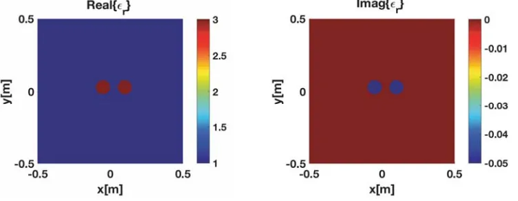
Figure 4. True complex permittivity profile.
The configuration for the first test problem is shown in Fig. 4 where we consider a target consisting of two circular lossy dielectric cylinders both having a radius of 5 cm. This target is placed off-center, towards the top-right corner of the imaging domain, which is chosen as a square region of 40 cm sides centered within the chamber. The cylinders are 5 cm apart and both have a complex permittivity of
r = 3−j0.05. The regularization of the problem was achieved using 1736 virtual test points located
outside the imaging domain. The location of these virtual test points is depicted in Fig. 3.
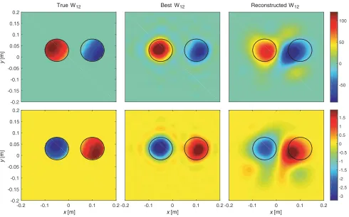
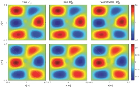
The reconstructed contrast sources associated with transmitter number 12, which is located at the point (−0.3,0.4) within the chamber, are shown in Fig. 5. These results are obtained at 550 MHz, which corresponds to a frequency that is well above the cut-off frequency for the chamber, ∼212 MHz. The left column shows the real and imaginary parts of the “True” contrast source, which are based on the numerically obtained total field from the DGM forward solver. The middle column is the “True” field expanded with the 625 eigenfunction basis; we denote this shows the “Best” representation in the chosen number of eigenfunctions. The reconstructed contrast source, using the same 625 eigenfunction basis, is shown in the right column. The black contours show the location of the cylinders in the forward model. Note that only the 40 cm square imaging domain is shown in these images.
True W12
-0.2 -0.15 -0.1 -0.05 0 0.05 0.1 0.15 0.2
-0.2 -0.1 0 0.1 0.2
-0.2 -0.15 -0.1 -0.05 0 0.05 0.1 0.15 0.2
Best W12
-0.2 -0.1 0 0.1 0.2
Reconstructed W12
-50 0 50 100
-0.2 -0.1 0 0.1 0.2
-3 -2.5 -2 -1.5 -1 -0.5 0 0.5 1 1.5
x [m]
y
[m]
y
[m]
x [m] x [m]
Figure 5. Real (top) and imaginary (bottom) of complex contrast source, w(r). From left to right: “True”: numerically obtained by the DGM forward solver, “Best”: expanded “True” profile with 625 eigenfunction basis, the reconstructedw(r) by recovering 625 unknown coefficients.
contrast source images compared to the “True” and “Best” images. The right most cylinder is reconstructed with a greater shift towards the center of the imaging domain than the left most cylinder. Numerical experiments indicate that this is due to the virtual point constraints being located closer to the right most cylinder. The constraints also seem to reduce the effect of Gibbs phenomenon in the reconstructions: we notice fewer oscillations in the reconstructed contrast sources compared to the “Best” representations using the same number of eigenfunctions.
Figure 6 presents the corresponding reconstructed scattered field. In Fig. 7 the real parts of the “Best” and reconstructed contrast-source and scattered-field coefficients are plotted. An increasing coefficient number generally indicates an increasing spatial frequency content of the eigenfunction although the ordering has not been chosen in such a way that the frequency content increases monotonically with the coefficient number. The plots clearly show that the scattered-field coefficients decay much faster than the contrast-source coefficients; the scattered-field coefficients quickly decay to almost zero while the contrast-source coefficients remain large even for coefficients associated with higher spatial frequency content. The low-pass filtering effect of the fundamental relation in Eq. (9), which relates contrast-source to scattered-field coefficients, is clearly evident. Higher spatial frequency information is not available in the scattered field, which constitutes the data for the inverse problem, and this contributes to the ill-posedness of the problem.
True Us12
-0.5 0 0.5
-0.5 0 0.5
-0.5 0 0.5
Best Us12
-0.5 0 0.5
Reconstructed Us12
-0.5 0 0.5
-0.5 0 0.5
-0.01 -0.005 0 0.005 0.01
x [m]
y
[m]
x [m] x [m]
y
[m]
Figure 6. Real (top) and imaginary (bottom) of complex scattered field, us(r). From left to right: “True”: numerically obtained by the DGM forward solver, “Best”: the expanded “True” scattered field with 625 eigenfunctions, the reconstructed us(r) by recovering 625 unknown coefficients.
according to the formula:
RMSE = F
Best−FRec
FBest (37)
whereFRec and FBestare, respectively, the reconstructed and the “Best” fields or their coefficients. Figure 8 shows the calculated RMSE using 25 to 625 eigenfunctions. The left plot, corresponding to the contrast source error, indicates that increasing the number of eigenfunctions to a certain point, 256, results in a continual reduction of the RMSE. Increasing N past 256 increases the error. This is quite different in the right plot, which corresponds to the scattered field, where the RMSE remains low after again reaching a minimum around 256. This, again, quantitatively illustrates the low-pass filtering effect of the fundamental relation in Eq. (9). It can be shown analytically that the relative errors in the contrast-source and scattered-field coefficients are identical, but because the high-frequency content of the scattered fields is much less than that of the contrast sources these relative errors contribute much more to the RMSE of the contrast sources.
4.1. Evaluation of the Two Regularization Schemes
To illustrate the remarkable impact that imposing virtual constraints has on regularizing the system matrix, we evaluate the algorithm’s performance under three different scenarios utilizing one or more of the four different sets of constraints depicted in Fig. 9. The number of virtual test points and contours for each constraint set are given in Table 1. For all three test scenarios, results for transmitter 12, depicted in Fig. 3, are reported but the results are independent of which transmitter is considered.
100 200 300 400 500 600
Coefficient Number
-2 -1.5 -1 -0.5 0 0.5 1 1.5 2
Best Real { w} Reconstructed Real { w}
100 200 300 400 500 600
Coefficient Number
-0.05 0 0.05 0.1 0.15 0.2 0.25
Reconstructed Real { s} Best Real { s}
Figure 7. Real part of the “Best” and reconstructed coefficients of contrast source (top) and scattered field (bottom).
(a) (b)
Figure 8. (a) RMSE of reconstructed contrast source and its corresponding coefficientsγw. (b) RMSE of reconstructed scattered field and its corresponding coefficients γs.
N. A larger N introduces higher spatial frequencies into the approximation and generally results in a more poorly conditioned system matrix leading to numerical instability in the approximated solution. Therefore, a trade-off between resolution and stability needs to be considered.
Constraint Set I Constraint Set II Constraint Set III Constraint Set IV
x [m]
y
[m]
-0.5 0 0.5
x [m]
-0.5 0 0.5
x [m]
-0.5 0 0.5
x [m]
-0.5 0 0.5
0.5 0.4 0.3 0.2 0.1 0 -0.5 -0.4 -0.3 -0.2 -0.1 0.5 0.4 0.3 0.2 0.1 0 -0.5 -0.4 -0.3 -0.2 -0.1 0.5 0.4 0.3 0.2 0.1 0 -0.5 -0.4 -0.3 -0.2 -0.1 0.5 0.4 0.3 0.2 0.1 0 -0.5 -0.4 -0.3 -0.2 -0.1
Figure 9. Different sets of constraints. Blue dots represent the virtual test points and red contours are the virtual contours.
100 200 300 400 500 600 Number of Eigenfunction Basis
30 25 20 15 10 0 5
log (cond(A A))
10
T
Before Regularization After Regularization
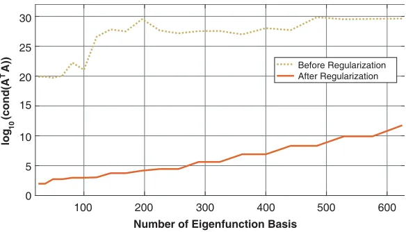
Figure 10. Condition number of matrix ATA for 25≤N ≤625 at 550 MHz using constraint Set III.
from the figure, for the same number of data points, increasing the eigenfunction expansion truncation number results in a higher condition number, however, by introducing the regularization we are able to considerably improve the condition numbers by an order of almost 1020, resulting in a stabilized well-conditioned solution.
Scenario Two: In this case, for a fixed number of data points and number of eigenfunctions, 40
and 625, respectively, the four different sets of virtual constraints are imposed to regularize the system matrix. The condition number of this matrix before regularization is 4.23×1029. The condition number
Table 1. Virtual constraints, number of constraint equations, and condition number ofATAat contrast source recovery stage of solving for 625 eigenfunction coefficients at 550 MHz. Constraint sets I, II, III and IV correspond to results presented in Fig. 11.
Constraint Virtual Test Points Virtual Contours Number of Constraint Equations A matrix size Initial Condition Number∗ Condition Number after Regularization
Set I 336 0 336 376×625 4.23×1029 1.87×10¹⁸
Set II 336 3 2211 2251×625 4.23×1029 2.66×10¹⁵
Set III 1736 0 1736 1776×625 4.23×1029 5.75×10¹¹
Set IV 8400 0 8400 8440×625 4.23×1029 1.74×10¹⁰
Best W 12
Reconstructed W12 with Constraint Set I
Reconstructed W12 with Constraint Set II
Reconstructed W12 with Constraint Set III
Reconstructed W12 with Constraint Set IV
-50 0 50 100 -3 -2 -1 0 1 2
x [m]
y [m] 0.2 0.1 0 -0.2 -0.1 0.2 0.1 0 -0.2 -0.1
x [m]
0.2 0.1 0 -0.2 -0.1
x [m]
0.2 0.1 0 -0.2 -0.1
x [m]
0.2 0.1 0 -0.2 -0.1
x [m]
0.2 0.1 0 -0.2 -0.1 y [m] 0.2 0.1 0 -0.2 -0.1 0.15 0.05 -0.05 -0.15
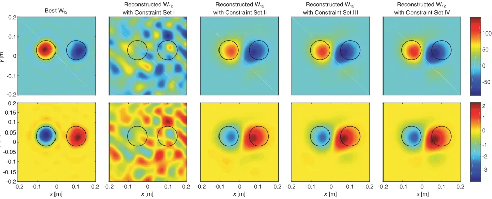
Figure 11. Real (top) and imaginary (bottom) parts of contrast source,w(r), when different constraint sets are imposed. From left to right: “Best”, reconstruction results, recovering 625 unknown coefficients, with constraint set I, II, III and IV shown in Fig. 9.
of the system matrix after imposing these constraint sets are shown in Table 1, which also includes the number of constraint equations that are added to the data equations. The reconstructed contrast sources for these four cases are shown in Fig. 11. It can be seen that when constraint Set I, consisting of only 336 virtual test points, is imposed, although the condition number has gone down from 4.23×1029 to 1.87×10¹⁸, the system matrix is not regularized to the point that accurate results can be reconstructed. By adding three square virtual contours to the 336 test points, that is, using constraint Set II, we add a total number of 2211(= 336 + 3×625) constraint equations, which results in a substantially reduced condition number of 2.66×10¹⁵. In other words, the result of concatenating these constraint equations to the data equations is to effectively create more linear independence between the columns of the system matrix, A, thereby reducing the condition number of the ATA matrix product. The result of imposing constraint Set III indicates that adding more virtual contours also leads to an improvement in the condition number.
Studying the algorithm’s performance for different combinations of constraints, it is observed that, for stabilizing the system, one has the choice of either imposing a large number of virtual test points or keeping the number of test points low and adding virtual contours. There was not a significant difference in the obtained results employing either of these techniques. However, the computational time for obtaining an inversion was generally found to be less when only virtual test points are imposed than when, in addition, one introduces virtual contours. This can be seen, e.g., for the case of Constraint Set III, where the number of constraint equations concatenated with the main data equations is less compared with imposing Constraint Set II. From the results of imposing Constraint Sets III and IV, it can be seen that although the number of virtual test points are almost 5 times more in Constraint Set IV than in III, the condition number has not changed significantly. The images in the two right-most columns of Fig. 11 provide confirmation that the improved condition number may not be warranted for this case. This also confirms the important fact that imposing too many virtual constraints does not have a negative impact on the contrast-source reconstruction.
Scenario Three: Now, the eigenfunction-based regularization approach is compared with the
0 100 200 300 400 500 600 -2
-1.5 -1 -0.5 0 0.5 1 1.5 2
-0.05 0 0.05
Coefficients Number
Coefficients Number
0 100 200 300 400 500 600
Real{γ }
Imag{γ }
W
W
Best
Eigenfunction-based Tikhonov SVD
Best
Eigenfunction-based Tikhonov SVD
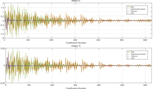
Figure 12. Real (top) and imaginary (bottom) parts of reconstructed contrast source coefficients of 625 eigenfunction basis at 550 MHz by means of eigenfunction-based, Tikhonov and SVD regularization methods.
coefficients are also included in this plot. It can be seen that all three regularization approaches result in comparable coefficients with the “Best” coefficients for a few first coefficients. However, the Tikhonov and SVD results are very small and close to zero for remaining coefficients. That is, the high spatial frequency details are suppressed. With eigenfunction-based regularization more non-zero coefficients are reconstructed. The resulting contrast source global profiles are illustrated in Fig. 13, which again confirms that the Tikhonov and SVD regularization approaches control the ill-posedness with the price of suppressing the higher spatial frequency components.
5. CONTRAST RECOVERY STAGE STUDY
The performance of the contrast recovery stage is studied next by presenting some numerical test cases for various targets. Utilizing the reconstructed contrast source coefficients for several interrogating fields one can form the well-conditioned matrix equation (34). We first present the recovered contrast profiles obtained when different virtual constraints are imposed for regularization as discussed in Section 4.1. Then for the test case introduced in Section 4, a separation resolution study similar to the one reported in [33] is conducted. We compare the eigenfunction inversion results with the results of a Discontinuous Galerkin Method Contrast Source Inversion (DGM-CSI) algorithm [36]. In addition, for the same test case and three other test cases, results of varying the truncation numberN are presented.
x [m] 0.2 0.1 0 -0.2 -0.1 y [m] 0.2 0.1 0 -0.2 -0.1 -50 0 50 100 -3 -2 -1 0 1 2 x [m] 0.2 0.1 0 -0.2 -0.1 x [m] 0.2 0.1 0 -0.2 -0.1 x [m] 0.2 0.1 0 -0.2 -0.1 y [m] 0.2 0.1 0 -0.2 -0.1
Best Eigenfunction-based Tikhonov SVD
Figure 13. Real (top) and imaginary (bottom) parts of contrast source profile, w(r), when different regularization methods are employed. From left to right: “Best”, eigenfunction-based regularization, Tikhonov regularization, SVD regularization.
Best (r)
Reconstructed (r) with Constraint Set I
Reconstructed (r) with Constraint Set II
Reconstructed (r) with Constraint Set III
Reconstructed (r) with Constraint Set IV
x [m]
0.2 0.1 0 -0.2 -0.1 y [m] 0.2 0.1 0 -0.2 -0.1 y [m] 0.2 0.1 0 -0.2 -0.1
x [m]
0.2 0.1 0 -0.2 -0.1
x [m]
0.2 0.1 0 -0.2 -0.1
x [m]
0.2 0.1 0 -0.2 -0.1
x [m]
0.2 0.1 0 -0.2 -0.1 3.5 3 2.5 2 1.5 1 0 -0.01 -0.02 -0.03 -0.04 -0.05 -0.06
Figure 14. Real (top) and imaginary (bottom) parts of permittivity, r(r), when different constraint sets are imposed. From left to right: “Best”, reconstruction results, recovering 625 unknown coefficients, with constraint set I, II, III and IV shown in Fig. 9.
5.1. Regularization Study
important observation that confirms that one has flexibility in choosing an appropriate virtual constraint set, with various sets producing acceptable results as compared to the “Best” obtainable solution. As was mentioned in Section 3, as long as regularization is achieved the only difference between these approaches is the required computational time.
5.2. Separation Resolution Study
The algorithm’s resolution performance is next quantified by performing a set of simple tests. One method of evaluating a MWI system’s performance is to measure its ability to resolve two dielectric targets, each of which individually produces a scattered field of similar strength, called the separation resolution [33, 37]. For MWI the separation resolution is target-dependent due to the nonlinearity of inverse scattering problem. However, this measure can provide a good indicator of the system’s performance. The separation resolution utilizes Rayleigh’s criterion as a metric for determining the performance of the system [38]. To determine if two targets are resolved, we consider the line connecting the centres of targets. Let Umin be the minimum reconstruction value between targets along the line
and Umax be the first maximum on the line closest to Umin. According to the Rayleigh’s criterion, the
targets are resolved if the ratioUmin/Umaxis less than 0.81.
The test case considered here consists of two circular cylinders each having a radius of 5 cm (∼λ/11, whereλis the free-space wavelength atf = 550 MHz). The two cylinders are placed off-center within the MWI system as depicted in Fig. 3. The background medium is free space and the complex permittivity of both objects is r = 3−j0.05. The separation between the two objects is varied from a maximum of λ/5 (∼ 11 cm) to a minimum of λ/60 (∼ 0.9 cm). The line in the image upon which the Rayleigh criterion is applied in the image is the line that passes through centers of two objects. Fig. 15 plots the resolution ratio that is obtained for all separation distances. In this plot the dashed line is the indicator of resolvability, 0.81. As can be seen, the algorithm was able to achieve the “Best” possible resolution of λ/45 in the image of the real part of the permittivity, whilst the resolution ratio in the image of the imaginary part of the permittivity was always below 0.81.
Figure 15. The resolution ratio of the real and imaginary parts.
The real and imaginary parts of the “Best” and reconstructed images with a separation ofλ/10 and
(a)
(b)
Figure 16. Real and imaginary parts of complex permittivity for two separation distances of 5.5 cm ∼ λ/10 and 1.6 cm ∼ λ/35. From left to right: “True”, “Best” (true permittivity expanded with 625 eigenfunctions), Reconstructed (results of NIEI using 625 coefficients, DGM-CSI after 150 iterations, (a) separation distance: 5.5 cm∼λ/10, (b) separation distance: 1.6 cm∼λ/35.
5.3. Eigenfunction Expansion Truncation Study
Contrast recovery performance is studied next for four test cases using different truncations of the eigenfunction basis,N = 121,225,361 and 625.
Figure 17. Test I — Real (first two rows) and imaginary (second two rows) of complex permittivity profile. “True” (left column), “Best” and reconstructed with 121, 225, 361 and 625 eigenfunctions (from second left column to right).
of the complex permittivity profile and the second set of two rows show the imaginary part. The first row in each set is the “Best” representation of “True” complex permittivity profile expanded with 121, 225, 361, and 625 eigenfunctions from left to right respectively, and the second row in each set shows the reconstructed images with 121, 225, 361, and 625 eigenfunctions, from left to right respectively. All reconstructions are obtained at 550 MHz. In general, there is good agreement between the best and reconstructed images for both the real and imaginary parts under different truncation numbers. A close look at the reconstructions reveals that increasing the truncation number not only helps one to obtain a better resolution by reconstructing coefficients for eigenfunctions containing higher spatial frequency information but also reconstructs the permittivity closer to the true value.
Similar to the results shown in Fig. 5, one can see the right most object is reconstructed with a greater shift towards the center of the imaging domain than the left most object, which is due to the fact that the virtual test point constraints are located closer to the right most object than the left most object.
Figure 18. Test II — Real (first two rows) and imaginary (second two rows) of complex permittivity profile. “True” (left column), “Best” and reconstructed with 121, 225, 361 and 625 eigenfunctions (from second left column to right).
This Forward model consists of two square cylinders, one with sides of 9 cm (∼λ/6) and one with sides of 7 cm (∼λ/8) at 550 MHz. As before free space is taken as the background medium. The larger square has a complex permittivity of r1 = 2−j0.05 while the smaller one has r2 = 1.3−j0.03. The real
and imaginary parts of the forward model, the “Best” and reconstructed permittivity profile images with 121, 225, 361 and 625 eigenfunctions are illustrated in Fig. 18. Similar observations can be made as in Test I, the reconstructed images for both the real and imaginary parts of the permittivity are comparable with the “Best” for different truncation numbers. It can be seen that reconstructing the smaller object having a smaller contrast is more difficult. This is expected due to the presence of the larger object that scatters greater electromagnetic energy.
Test III — same size adjacent circular cylinders with same electrical properties embedded in third
medium: This model includes two circular cylinders, each having a radius of 5 cm and complex
permittivity of r1 = 3−j0.05, that are bounded by a third circular cylinder having a radius of
15 cm placed off-center with respect to the two interior cylinders. The outer embedding cylinder has a complex permittivity of r2 = 1.4−j0.01. The background medium is again free space and the test is
Figure 19. Test III — Real (first two rows) and imaginary (second two rows) of complex permittivity profile. “True” (left column), “Best” and reconstructed with 121, 225, 361 and 625 eigenfunctions (from second left column to right).
As can be observed from the results shown in Fig. 19, Test III is a more challenging inverse problem compared with Test I which contained only the interior cylinders. However, the NIEI algorithm is able to resolve the two circular targets within the third medium.
Test IV — diagonally-oriented different sized circular cylinders with different electrical properties
embedded in a third medium: This model consists of two circular cylinders having radii of 4 cm and
3.5 cm, placed off-center and diagonally oriented. These two cylinders are enclosed by a third circular cylinder having a radius of 15 cm, which itself is placed off center in the chamber. Complex permittivities of r1 = 2.1−j0.05 and r2 = 1.6−j0.03 are considered for the two inner cylinders, and a complex
Figure 20. Test IV — Real (first two rows) and imaginary (second two rows) of complex permittivity profile. “True” (left column), “Best” and reconstructed with 121, 225, 361 and 625 eigenfunctions (from second left column to right).
Figure 21. Test I — RMSE of the real and imaginary parts of reconstructed contrast and its corresponding coefficients, γχ, at 550 MHz.
6. DISCUSSION
A unique feature of the NIEI algorithm is that it does not require a mesh for discretizing the spatial domain and it can be developed fully analytically for chambers having a canonical shape. That is, the eigenfunctions can be written analytically. Thus, the only numerical approximation involved consists of truncating the expansions. This automatically introduces a level of regularization into the inversion algorithm. This fact was reported in [32], and is effective because of the removal of higher spatial frequencies from consideration which cannot be reconstructed using only information obtained from scattered field data. The low-pass filtering of the inverse-source operator means that high spatial frequency information of the contrast sources just isn’t available in the scattered field.
The unique regularization technique of constraining the contrast sources to be zero outside the imaging domain is enabled because of the use of a whole-domain basis. Such a technique could not be formulated on a mesh. It effectively adds new virtual information that dramatically improves the condition number of the system matrix and enables one to solve the inverse-source problem non-iteratively. Via the derived fundamental relation between the scattered field and contrast source coefficients, Equation (9), this virtual information regarding the contrast sources is transferred to the scattered field (which is not zero outside the imaging domain).
The results of inverting several relatively difficult test cases confirm the algorithm’s ability to recover both contrast sources and contrast profiles with a high level of accuracy in the lower spatial frequencies of the problem, when compared to the “True” and “Best” profiles. For the test case shown in Section 5.3, the algorithm was able to resolve two objects as close as λ/45. This is a very high level of resolution in MWI and comparable to that obtainable using a state-of-the-art imaging algorithm like the Finite-Element Contrast Source Inversion (FEM-CSI) algorithm [39]. This achievement is most remarkable because the NIEI algorithm is non-iterative, making it very efficient.
25 36 49 64 81 100 121 144 169 196 225 256 289 324 361 400 441 484 529 576 625 Number of Eigenfunction Basis
400
350
300
250
200
150
100
50
0
Time (sec)
Build Up Time
Run Time
Figure 22. “Build Up Time” and “Run Time” for different numbers of eigenfunction basis.
7. CONCLUSION
The NIEI algorithm was introduced, which consists of two non-iterative inversion stages: (1) solving a series of inverse-source problems and (2) combining the inverse source results into a contrast recovery stage. The algorithm was demonstrated for the 2D Helmholtz BVP formulation of quantitative MWI using a conductive imaging chamber. The algorithm expands the unknown functions using the eigenfunctions for the Helmholtz BVP as a whole-domain basis. An innovative regularization approach that constrains the contrast sources to be zero outside the imaging domain at virtual test points or virtual contours results in well-conditioned inverse-source system matrices that are efficiently inverted in a least-squares sense. The algorithm’s performance was assessed using several numerical studies and the results clearly demonstrate the algorithm’s robustness and applicability to difficult inversion problems.
The computational resources required by the algorithm are extremely low and cutting-edge in terms of the state-of-the-art for inverse problems. The algorithm is easily extendible to 3D imaging applications and it is expected that the computational resource savings will be even more competitive with existing state-of-the-art 3D inversion techniques. Future research related to extending the algorithm to the case of 3D imaging using 3D vector-field data has already begun [40]. Such a 3D eigenfunction-based non-iterative inversion algorithm is expected to be significantly faster than previously reported 3D MWI techniques.
ACKNOWLEDGMENT
This work was supported by the Canadian Cancer Society, grant number 300028.
REFERENCES
2. Yemelyanov, K. M., N. Engheta, A. Hoorfar, and J. A. McVay, “Adaptive polarization contrast techniques for through-wall microwave imaging applications,” IEEE Transactions on Geoscience and Remote Sensing, Vol. 47, No. 5, 1362–1374, 2009.
3. Woodhouse, I. H., Introduction to Microwave Remote Sensing, CRC Press, 2017.
4. Wagner, W., G. Bloschl, P. Pampaloni, J.-C. Calvet, B. Bizzarri, J.-P. Wigneron, and Y. Kerr, “Operational readiness of microwave remote sensing of soil moisture for hydrologic applications,”
Nordic Hydrology, Vol. 38, No. 1, 1–20, 2007.
5. Chandra, R., H. Zhou, I. Balasingham, and R. M. Narayanan, “On the opportunities and challenges in microwave medical sensing and imaging,”IEEE Transactions on Biomedical Engineering, Vol. 62, No. 7, 1667–1682, 2015.
6. Fear, E. C., X. Li, S. C. Hagness, and M. A. Stuchly, “Confocal microwave imaging for breast cancer detection: Localization of tumors in three dimensions,”IEEE Transactions on Biomedical Engineering, Vol. 49, No. 8, 812–822, 2002.
7. Beada’a, J. M., A. M. Abbosh, S. Mustafa, and D. Ireland, “Microwave system for head imaging,”
IEEE Transactions on Instrumentation and Measurement, Vol. 63, No. 1, 117, 2014.
8. Mojabi, P. and J. LoVetri, “Eigenfunction contrast source inversion for circular metallic enclosures,”
Inverse Problems, Vol. 26, No. 2, 025010, 2010.
9. Gilmore, C. and J. LoVetri, “Enhancement of microwave tomography through the use of electrically conducting enclosures,” Inverse Problems, Vol. 24, No. 3, 035008, 2008.
10. Nemez, K., A. Baran, M. Asefi, and J. LoVetri, “Modeling error and calibration techniques for a faceted metallic chamber formagnetic field microwave imaging,”IEEE Transactions on Microwave Theory and Techniques, Vol. 65, No. 11, 4347–4356, 2017.
11. Pastorino, M., Microwave Imaging, Vol. 208, John Wiley & Sons, 2010.
12. Chen, X., Computational Methods for Electromagnetic Inverse Scattering, Wiley Online Library, 2018.
13. De Zaeytijd, J., A. Franchois, C. Eyraud, and J.-M. Geffrin, “Full-wave three-dimensional microwave imaging with a regularized Gauss-Newton method — Theory and experiment,” IEEE Transactions on Antennas and Propagation, Vol. 55, No. 11, 3279–3292, 2007.
14. Souvorov, A. E., A. E. Bulyshev, S. Y. Semenov, R. H. Svenson, A. G. Nazarov, Y. E. Sizov, and G. P. Tatsis, “Microwave tomography: A two-dimensional newton iterative scheme,” IEEE Transactions on Microwave Theory and Techniques, Vol. 46, No. 11, 1654–1659, 1998.
15. Rubæk, T., P. M. Meaney, P. Meincke, and K. D. Paulsen, “Nonlinear microwave imaging for breast-cancer screening using Gauss-Newton’s method and the CGLS inversion algorithm,” IEEE Transactions on Antennas and Propagation, Vol. 55, No. 8, 2320–2331, 2007.
16. Harada, H., D. J. Wall, T. Takenaka, and M. Tanaka, “Conjugate gradient method applied to inverse scattering problem,” IEEE Transactions on Antennas and Propagation, Vol. 43, No. 8, 784–792, 1995.
17. Franchois, A. and A. Tijhuis, “A quasi-Newton reconstruction algorithm for a complex microwave imaging scanner environment,” Radio Science, Vol. 38, No. 2, 1–12, 2003.
18. Kleinman, R. and P. van den Berg, “A modified gradient method for two-dimensional problems in tomography,”Journal of Computational and Applied Mathematics, Vol. 42, No. 1, 17–35, 1992. 19. Caorsi, S., A. Massa, M. Pastorino, and A. Rosani, “Microwave medical imaging: Potentialities
and limitations of a stochastic optimization technique,” IEEE Transactions on Microwave Theory and Techniques, Vol. 52, No. 8, 1909–1916, 2004.
20. Colton, D. and R. Kress,Inverse Acoustic and Electromagnetic Scattering Theory, Vol. 93, Springer Science & Business Media, 2012.
21. Tikhonov, A. N., “Solution of incorrectly formulated problems and the regularization method,”
Soviet Math. Dokl., Vol. 4, 1035–1038, 1963.
23. Xu, P., “Truncated SVD methods for discrete linear ill-posed problems,” Geophysical Journal International, Vol. 135, No. 2, 505–514, 1998.
24. Hansen, P. C., “Regularization, GSVD and truncated GSVD,” BIT Numerical Mathematics, Vol. 29, No. 3, 491–504, 1989.
25. Hansen, P. C., T. Sekii, and H. Shibahashi, “The modified truncated SVD method for regularization in general form,”SIAM Journal on Scientific and Statistical Computing, Vol. 13, No. 5, 1142–1150, 1992.
26. Hansen, P. C., “Analysis of discrete ill-posed problems by means of the L-curve,” SIAM Review, Vol. 34, No. 4, 561–580, 1992.
27. Hansen, P. C. and D. P. O’Leary, “The use of the L-curve in the regularization of discrete ill-posed problems,” SIAM Journal on Scientific Computing, Vol. 14, No. 6, 1487–1503, 1993.
28. Mojabi, P. and J. LoVetri, “Overview and classification of some regularization techniques for the Gauss-Newton inversion method applied to inverse scattering problems,” IEEE Transactions on Antennas and Propagation, Vol. 57, No. 9, 2658–2665, 2009.
29. Scapaticci, R., I. Catapano, and L. Crocco, “Wavelet-based adaptive multiresolution inversion for quantitative microwave imaging of breast tissues,” IEEE Transactions on Antennas and Propagation, Vol. 60, No. 8, 3717–3726, 2012.
30. Scapaticci, R., P. Kosmas, and L. Crocco, “Wavelet-based regularization for robust microwave imaging in medical applications,” IEEE Transactions on Biomedical Engineering, Vol. 62, No. 4, 1195–1202, 2015.
31. Winters, D. W., J. D. Shea, P. Kosmas, B. D. van Veen, and S. C. Hagness, “Three-dimensional microwave breast imaging: Dispersive dielectric properties estimation using patient-specific basis functions,”IEEE Transactions on Medical Imaging, Vol. 28, No. 7, 969–981, 2009.
32. Grote, M. J., M. Kray, and U. Nahum, “Adaptive eigenspace method for inverse scattering problems in the frequency domain,”Inverse Problems, Vol. 33, No. 2, 025006, 2017.
33. Gilmore, C., P. Mojabi, A. Zakaria, S. Pistorius, and J. LoVetri, “On super-resolution with an experimental microwave tomography system,” IEEE Antennas and Wireless Propagation Letters, Vol. 9, 393–396, 2010.
34. Asefi, M., G. Faucher, and J. LoVetri, “Surface-current measurements as data for electromagnetic imaging within metallic enclosures,” IEEE Transactions on Microwave Theory and Techniques, Vol. 64, No. 11, 4039–4047, 2016.
35. Jeffrey, I., A. Zakaria, and J. LoVetri, “Microwave imaging by mixed-order discontinuous Galerkin contrast source inversion,”2014 XXXIth URSI General Assembly and Scientific Symposium (URSI
GASS), 1–4, IEEE, 2014.
36. Jeffrey, I., N. Geddert, K. Brown, and J. LoVetri, “The time-harmonic discontinuous Galerkin method as a robust forward solver for microwave imaging applications,” Progress In Electromagnetics Research, Vol. 154, 1–21, 2015.
37. Den Dekker, A. and A. van den Bos, “Resolution: A survey,” JOSA A, Vol. 14, No. 3, 547–557, 1997.
38. Born, M., E. Wolf, A. B. Bhatia, et al., Principles of Optics: Electromagnetic Theory of Propagation, Interference and Diffraction of Light, Vol. 7, Cambridge University Press, Cambridge, 1999.
39. Zakaria, A., C. Gilmore, and J. LoVetri, “Finite-element contrast source inversion method for microwave imaging,” Inverse Problems, Vol. 26, No. 11, 115010, 2010.
40. Abdollahi, N., I. Jeffrey, and J. LoVetri, “A non-iterative eigenfunction-based 3D inverse solver for microwave imaging,” Second URSI Atlantic Radio Science Meeting Science General Assembly