Comparison of Algorithms and Input Vectors for Sea-Ice Classification with L-Band PolSAR Data

(1)

Comparison of Algorithms and Input Vectors for Sea-Ice

Classification with L-Band PolSAR Data

Kai-Shiun Yang and Jean-Fu Kiang*

Abstract—Two unsupervised methods, fuzzyc-means (FCM) andk-means, as well as three supervised methods, support vector machine (SVM), neural network (NN), and convolutional neural network (CNN), are applied to classify sea-ice type of first-year ice (FYI), multi-year ice (MYI) and open water, by using L-band polarimetric synthetic aperture radar (PolSAR) images in winter and advanced-melt phases, respectively. Different input vectors, pending on different scenarios, are also proposed to increase the accuracy rate. The efficacy of different algorithms in conjunction with different input vectors are analyzed and related to the underlying physical mechanisms.

1. INTRODUCTION

The status of Arctic sea-ice coverage has been closely watched as a critical task of tracking global warming and climate change. Variation of sea-ice thickness and extent over 2000–2012 was analyzed by using satellite and airborne data [1, 2]. Sea ice can be roughly classified into first-year ice (FYI) and multi-year ice (MYI) [3]. During the summer, FYI melts, MYI recedes, and two-year or three-year sea-ice replace their predecessor. Existing MYI is usually thicker than FYI and is easier to survive the summer [4]. The open water surrounding sea-ice absorbs more heat than the sea-ice itself, which accelerates the melting process [2]. Recession of sea ice makes marine transportation across the Arctic more attractive [2, 5]. However, misclassified thick MYI during the melting season may pose navigation hazards [6].

Synthetic aperture radar (SAR) has been used to monitor and classify Arctic sea-ice [7, 8]. The Canadian Ice Service (CIS) compiles sea-ice chart by using RADARSAT and other auxiliary data [9]. In [10], previous researches on sensing snow and sea ice with electromagnetic waves were reviewed. Scattering models of MYI and FYI at different temperatures and roughness conditions were summarized. Field measurements indicate that different types of sea ice cast different radar signatures. The backscattering power varies with sea-ice type, surface roughness, snow cover and melting pool [11– 13].

The radar signature of sea ice appears different at different electromagnetic wavelengths. In C-band polarimetric synthetic aperture radar (PolSAR) imaging, backscattering from FYI is dominated by surface scattering, while that from MYI is dominated by volume scattering [10]. Field measurements show that MYI is prone to enclose more air bubbles that FYI is, and shorter electromagnetic wavelength is more sensitive to the air bubbles within the weathered surface layer [14]. Satellite observation of landfast ice showed that the difference of σvv between MYI and FYI was greater than 3 dB during the winter [13]. As compared to C-band imaging, the contrast between MYI and FYI is not as distinct in the L-band. L-band and X-band waves are sensitive to roughness of dm-scale and cm-scale, respectively [15]. The backscattering power in C-band from frost-flower, which is of cm-scale, is on the same order as that from MYI [5, 16], but the backscattering power in L-band from frost-flower is far weaker than that from MYI.

Received 4 January 2019, Accepted 25 March 2019, Scheduled 2 April 2019

* Corresponding author: Jean-Fu Kiang ([email protected]).

(2)

The pros and cons of using L-band and C-band radars for sea-ice monitoring were reviewed in [7]. Co-located PolSAR images in L-band and C-band were compared to study the difference of their radar signatures [7, 17]. In [18], radar signatures of newly formed sea-ice in L, C and X-bands were presented. Sea-ice deformation such as ridges, rubble fields or brash ice can be detected more accurately in L-band than in C-L-band. Polarimetric features such as polarimetry entropy [19] and co-polarization ratio, were used to classify among open water, new ice, smooth ice, and deformed ice. C-band PolSAR backscattering data were validated by field measurements for sea-ice classification [20, 21] and proved effective in identifying the extent of MYI in the winter [5].

Both supervised and unsupervised methods have been applied to classify pixels in PolSAR images into different features. Examples of supervised methods include neural network (NN) [8], support vector machine (SVM) [22], convolutional NN (CNN) [23] and autoencoder [24]. Examples of unsupervised methods include Wishart classifier [25, 26], fuzzy c-means (FCM) [27, 28], as well as expectation maximization algorithm with log-cumulants [29] and Wishart classifiers [25]. Gray-level co-occurrence matrices (GLCMs) were used as input data to a supervised Bayesian classifier for analyzing sea-ice texture [30] as well as to an NN algorithm for generating classified ice map [8]. In [22], an SVM classifier was trained with input data of backscattering power and GLCM. In [31], preprocessed polarimetric parameters were used as input data to an NN algorithm to classify sea-ice into open water (OW), young ice, smooth FYI and rough FYI/MYI. In [32], a hybrid crop classifier on PolSAR images was proposed. The input vector is composed of span, H/A/α decomposition parameters and GLCM-based features. A two-hidden-layer forward NN was constructed and trained by using adaptive chaotic particle swarm optimization (ACPSO). In [33], an 11-layer deep CNN was applied for PolSAR image segmentation on L-band data over the San Francisco bay area and C-band data over Flevoland area.

In this work, we study the performance of some popular supervised and unsupervised methods in classifying sea-ice type, with the input data of full-polarimetric ALOS PALSAR (L-band) images. Several forms of input vector are proposed, by exploiting features embedded in L-band PolSAR images, to increase the accuracy rate of sea-ice classification in the winter phase and the advanced-melt phase, respectively. This work is organized as follows. The radar signatures of sea ice are briefly reviewed in Section 2, the images and input vectors for classification are presented in Sections 3 and 4, respectively, the classification methods are briefly reviewed in Section 5, the simulation results are discussed in Section 6, and some conclusions are drawn in Section 7.

2. RADAR SIGNATURES OF SEA ICE

In this Section, general features of sea ice and its radar signatures in L-band and C-band are brieﬂy reviewed. There are three distinct types of scattering phenomena from sea surface [34]. The ﬁrst one is Bragg scattering from resonant capillary waves at moderate wind speed, the second one is burst scattering from the wave crests just before break [34], and the third one is white-cap scattering from very rough surface as wave crests break, at wind speed higher than 20 m/s [35]. The co-polarization ratio of radar cross-sections (RCSs),σvv/σhh, of Bragg scattering from sea surface appears independent

of ocean-wave spectrum [36]. Newly formed sea-ice under calm weather condition tends to damp sea waves, reducing the backscattering power [18].

In general, undeformed surface of FYI is ﬂat, and the surface of MYI is rough [10]. The melting water from sea ice freezes up after contacting the snow, forming a rough ice layer on top of snow, in the early melting phase [37]. Refrozen melting pools formed in advanced-melt phase make the second-year ice rougher than FYI.

The radar signatures of sea ice in C-band and L-band are diﬀerent [5, 7, 13, 17]. The dominant scattering mechanism of MYI is volume scattering in C-band and surface scattering in L-band [13]. The volume scattering comes from the upper layer of MYI, which has low salinity and encloses air bubbles [10]. A C-band scattering experiment on FYI [38] reported that rough-surface scattering dominates at low incidence angle, volume scattering from snow is less signiﬁcant, and wet snow decreases volume scattering.

(3)

appears on top of young ice, appears similar to that of MYI [16].

3. IMAGES FOR CLASSIFICATION

The states of sea ice can be categorized, in terms of radar signature, into five different phases, winter, early melt, melt onset, advanced-melt, and freeze-up [39]. The images in the winter phase (dry snow-pack on dry sea-ice, with surface temperature below −5◦C) and the advanced-melt phase (snow pack is wet and melts rapidly) will be classified and analyzed in this work.

3.1. Winter Phase

Figure 1(a) shows the C-band image of σvv in Beaufort sea near Northwest Canadian coastline in

the winter phase. Two regions of interest (ROIs) are enclosed by red boxes and labeled by 1 and 2, respectively. L-band full-polarimetry images are also available in these two ROIs. Table 1 lists the ice concentration in zones A and B, respectively, from CIS sea-ice chart [40]. During these two days of data acquisition, ice ﬂoes slightly moved south-eastwards. Note that the zone types shown in Fig. 1(a) and the ice concentration listed in Table 1 were recorded on April 23 and April 30, 2007.

(a) (b)

Figure 1. C-band image of σvv: (a) In Beaufort sea near Northwest Canadian coastline, recorded on

April 27, 2007 (winter). ROI 1 and ROI 2 are enclosed by red boxes, purple and yellow curves mark boundaries between zone A and zone B on April 23 and April 30, 2007, respectively, on Canadian Ice Service (CIS) sea-ice chart [40]. (b) Between Melville Island and Banks Island, Canada, recorded on August 11, 2009 (advanced-melt). ROI 3 is enclosed by red box, blue curves mark boundaries between zone A’ and zone B’ on August 10, 2009, on CIS sea-ice chart.

Figure 2 shows theσvvimages in L-band and C-band, respectively, in the winter phase. The C-band images ofσvvwere taken with the Remote-Sensing Satellite-2 (ERS-2) of European Space Agency (ESA) at UTC 06:16–06:18, April 27, 2007, and the data are retrieved from the ESA EO data collections [41]. The L-band images of σvv were taken with the Advanced Land Observing Satellite (ALOS) Phased

(4)

Table 1. Ice concentration in zones A, B, A’ and B’ [40].

zone A zone B

FYI(a) MYI(b) FYI(a) MYI(b)

concentration 8 2 5 5

zone A’ zone B’

FYI(a) thick FYI(c) open water thick FYI(c)

concentration 1 9 5 5

sum of concentrations is 10 in one zone. (a): ice thickness 30–70 cm, (b): old ice, (c): ice thickness

>120 cm.

(a) (b)

(c) (d)

Figure 2. L-band image ofσvv in (a) ROI 1 and (b) ROI 2. C-band image ofσvv in (c) ROI 1 and (d) ROI 2. Data not available in light-blue areas.

Table 2 lists some system parameters of the ALOS PALSAR and ERS-2, respectively. The geometrical area of both ROI 1 and ROI 2 is 29 km ×65 km. Both images in Figs. 2(a) and 2(b) are composed of 624 horizontal rows, with 4,608 pixels in each row. The size of each pixel is 46 m (row width) ×14 m.

It is observed that ridges appear more clearly in L-band images than in C-band images, consistent with the observations in [7]. The boundary of MYI appears more clearly in C-band images than in L-band images, consistent with the observations in [13]. By comparing the two areas enclosed by red curves in Figs. 2(a) and 2(c), we observe that the σvv appears dark in L-band and light in C-band,

probably caused by the frost ﬂower on ice.

(5)

Table 2. Parameters of ALOS PALSAR [43] and ERS-2 [44, 45].

unit ALOS PALSAR ERS-2

polarization hh/vh/hv/vv vv

noise equivalent sigma zero (NESZ) dB −29 −23

center frequency GHz 1.270 5.3

wavelength m 0.2379 0.056

bandwidth MHz 14 15.55

incidence angle degree 8–30 20.1–25.9

ground swath km 30 100

mechanisms [46]. It appears that most of the scatterers belong to Bragg surface and random surface, respectively. Fig. 3(b) shows that the polarimetry entropy of FYI is relatively higher than that of MYI. High polarimetry entropy implies low scattering signal-to-noise ratio (SNR), and the pixels with SNR

<6 dB [47] are marked black in Fig. 3(c). An oil-spill sea surface reveals similar characteristics of weak scattering, low SNR or high entropy [48].

(a) (b) (c)

Figure 3. Properties of L-band image in ROI 1, (a) PDF inH/α plane, (b) polarimetry entropy H, (c) pixels with SNR <6 dB are marked black.

3.2. Advanced-Melt Phase

Figure 1(b) shows the C-band image of σvv between Melville Island and Banks Island, Canada, in

advanced-melt phase. The ROI is enclosed with red box and labeled by 3. L-band full-polarimetry image is also available in ROI 3. Table 1 lists the ice concentrations in zones A’ and B’ on August 10, 2009, from CIS sea-ice chart [40]. The ERS-2 (C-band) image was taken at UTC 05:00 August 11, 2009, and the ALOS PALSAR (L-band) image was taken at UTC 04:33 August 11, 2009.

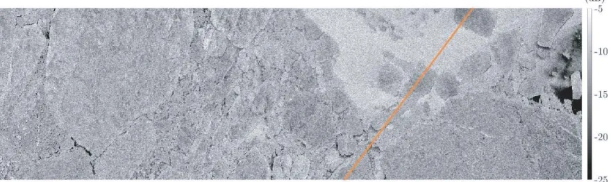
Figure 4 shows the L-band image ofσvv in ROI 3, of which the geometrical area is 29 km×121 km. The image is composed of 624 horizontal rows, with 8,509 pixels in each row. The size of each pixel is 46 m (row width) ×14 m.

Figure 5(a) shows the PDF of the L-band image in theH/αplane, where two clusters are observed. By inspecting Fig. 4, we observe open-water areas in the right-half image but none in the left-half one. Hence, we split the image of Fig. 4 into left half and right half. Figs. 5(b) and 5(c) show the PDFs in the H/α plane, of the left-half image and the right-half image, respectively. There are two distinct types of scatterer in the right-half image, corresponding to sea ice and open water, respectively.

Figure 5(d) shows the polarimetry entropy of the whole image, with low-entropy pixels and high-entropy pixels mapped to the two clusters of PDF, respectively, in Fig. 5(a). About 50% of pixels on the right-half image represent open-water area, which are expected to have relatively low entropy. Fig. 5(f) shows the PDF in the (H, σvv/σhh) plane, where two distinct clusters are observed, consistent with the

(6)

Figure 4. L-band image ofσvv in ROI 3, C-band image not available to the right of orange line.

(a) (b) (c)

(d) (e) (f)

Figure 5. Properties of L-band image in Fig. 4, (a) PDF of whole image in H/α plane, (b) PDF of left-half image inH/αplane, (c) PDF of right-half image inH/α plane, (d) polarimetry entropyH, (e) co-polarization ratio σvv/σhh, (f) PDF of whole image in (H, σvv/σhh) plane.

Figure 6 shows the co-polarization ratioσvv/σhh of open water versus incidence angle [36], which

is consistent with Fig. 5(e) that areas with σvv/σhh>2 are very likely open water.

3.3. Reference Ground-Truth

The backscattering coeﬃcients (BSCs) have been used to classify MYI and FYI. It was reported that the measured σvv of smooth FYI was lower than −15 dB, and that of rough FYI and second-year ice was about−13 dB [11];σvvof snow-free MYI was higher than−10 dB, and the diﬀerence ofσvv between

snow-covered FYI and snow-free MYI was larger than 3 dB [12]. The satellite observation of landfast ice showed that the diﬀerence of σvv between MYI and FYI was larger than 3 dB in the winter [13].

Typical look angle of scattered ﬁeld in measurements is about 25◦.

(7)

Figure 6. Co-polarization ratioσvv/σhh versus incidence angle [36], relative permittivity of sea water

isr= 76−j48 [49] at 1.413 GHz and 35 psu of salinity.

observation confirmed that C-band SAR images from ERS-2 and RADARSAT could effectively classify flaw polynya, new ice, FYI and MYI. In [7], co-located C-band SAR images were used to confirm the sea-ice classification by using L-band SAR images, based on previous studies in [20, 21]. The relation between C-band backscattering power and sea-ice type was reviewed by summarizing data from the literature, including open water, nilas, young ice, level FYI, deformed FYI and MYI [8].

Based on these discussions, a ﬂowchart of preparing the reference ground-truth is proposed, as shown in Fig. 7. Three classiﬁcation labels, OW, FYI and MYI, are chosen. The following rules are applied in sequence.

1) Check sea-ice type in the ROI from sea-ice chart.

2) If water exists, classify a pixel into open water or FYI, by usingHandσvv/σhhderived from L-band

image.

3) If water does not exist, use relative backscattering power of C-band image to classify into FYI or MYI. Classify a pixel into MYI if the power is strong and FYI if the power is weak.

4) If the backscattering power of a pixel appears strong in C-band but weak in L-band, indicating coverage with frost ﬂower, then classify the pixel into FYI.

Figure 7. Flowchart of preparing reference ground-truth.

4. INPUT VECTORS

(8)

(τ) as [50] ¯ ¯ C= ⎡ ⎢ ⎢ ⎣

|Shh|2 √2ShhShv∗ ShhSvv∗

√

2S_hh∗ Shv 2|Shv|2 √2ShvSvv∗

ShhSvv∗

√

2S_hv∗ Svv |Svv|2

⎤ ⎥ ⎥

⎦=τW¯¯ (1)

where ¯W¯ follows a Wishart distribution.

The ﬁrst three log-cumulants of covariance matrix ¯C¯ of a target pixel are deﬁned as [51]

κ1{C¯¯} = μ1{C¯¯}, κ2{C¯¯}=μ2{C¯¯} −μ21{C¯¯}

κ3{C¯¯} = μ3{C¯¯} −3μ1{C¯¯}μ2{C¯¯}+ 2μ31{C¯¯}

representing mean, variance, and skewness, respectively, in the log domain [52], which have been used to classify diﬀerent ground or sea-surface features. Here,μn{C¯¯}= _M1 M=1 ln

det{C¯¯}

_n

[51], where ¯

¯

Cis the covariance matrix associated with a pixel in the neighborhood of the target pixel. In this work,

a neighborhood is composed ofM = 9 pixels, with three rows in the range direction and three pixels in each row.

Diﬀerent land covers, like ground, vegetation, and roof in urban area, form distinct clusters in the (κ3, κ2) plane [53]. Oil-spill and sea water form distinct clusters in the (κ1, κ2) plane, but less distinct

clusters in the (κ3, κ2) plane [54]. The PDF of Polynya, brash/pancake ice and white ﬂoe in C-band

polarimetric images formed diﬀerent clusters in the (β1, β2) plane [55]. The analysis on PDF of PolSAR

images was simpliﬁed in the (κ3, κ2) plane than in the (β1, β2) plane [52]. The surface properties of FYI

and MYI are more complicated than sea water in L-band images, hence log-cumulants are considered as constituents of input vector for FYI/MYI classiﬁcation.

GLCM features have been used for sea-ice classiﬁcation [8, 22, 30]. Commonly used GLCM features includef1(energy),f2 (contrast),f3 (homogeneity) andf4 (entropy). The contrast featuref2 measures

the intensity contrast around the target pixel, which could be useful in classifying FYI and MYI, as deformed FYI reveals black-and-white chequered texture of high contrast while plain FYI and MYI reveal low contrast.

Classifiers like NN, SVM, FCM, andk-means cannot generate texture information by themselves. Including texture information of images may increase the accuracy rate of these classifiers. As shown in Figs. 3(a) and 5(a), most scatterers are clustered to a small zone, implying that they are dominated by the same type of scattering mechanism and are difficult to separate by using the information in ¯C¯

alone. The GLCM features are included to enhance the classiﬁers. Here, we propose two types of input vector,

[κ1, κ2, f2]t (2)

[κ1, κ2, f2, H, σvv/σhh]t (3)

which include information of texture and scattering mechanism. These input vectors will be used for classiﬁcation methods NN, SVM, FCM and k-means. Fig. 5(f) shows that open water can be clearly identiﬁed in the H-σvv/σhh plane, hence the input vector of (3) is expected to perform better when

open water exists.

In deep-learning models for PolSAR terrain classiﬁcation [23, 24, 56], all elements in the covariance matrix ¯C¯ of a pixel are rearranged into a 9-element input vector as

¯

C =

|Shh|2,|Shv|2,|Svv2 |,Re{ShhShv∗ },Im{ShhShv∗ },Re{ShhSvv∗ },Im{ShhSvv∗ },

Re{ShvSvv∗ },Im{ShvSvv∗ }

_t

(4)

To reduce the complexity of CNN while retaining important polarimetric information, an alternative input vector is deﬁned as

[κ1, κ2]t (5)

(9)

5. REVIEW OF CLASSIFICATION METHODS

Typical supervised method takes a large quantity of training data to achieve acceptable accuracy rate [57]. On the other hand, unsupervised methods do not require training data at all, making them useful when ground-truth data are diﬃcult to acquire. In this work, sea ice will be classiﬁed with supervised methods (NN, CNN and SVM) and unsupervised methods (k-means and FCM), respectively. The accuracy rate of these methods will be compared and analyzed.

5.1. Supervised Methods

In [8], an NN method was proposed to classify sea ice into water, level FYI, deformed FYI and MYI, by using GLCM features as the input vector. The NN was composed of three layers, containing 9, 6 and 3 neurons, respectively. In [58], an NN was proposed to classify pixels of C-band and L-band images, respectively, into open water, thin ice/calm water and sea ice. The ground-truth was manually determined on backscattering power and texture features. The input vector contains σhh,

σhv, autocorrelation ofσhv (a GLCM texture feature), incidence angle andσhv/σhh. The proposed NN

was composed of three layers, with 5 neurons in the input layer and 3 neurons in the output layer. Figure 8 shows the schematic of a conventional NN, which is composed of three fully-connected hidden layers, containing 20, 30, and 10 neurons, respectively. It processes one pixel at a time in both the training phase and the testing phase.

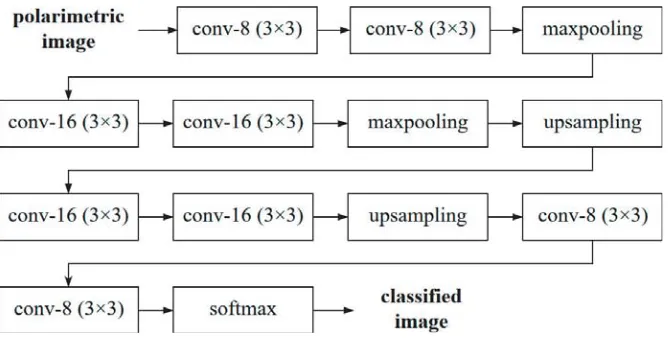
Figure 9 shows the schematic of CNN used in this work, which is modiﬁed from SegNet [59], where conv-n (3, 3) means a convolutional layer which is composed of n ﬁlters of size 3×3, followed by a ReLU activation function and batch normalization; maxpooling means choosing the maximum value

Figure 8. Schematic of conventional NN.

(10)

from every 2×2 pixels; upsampling means duplicating a single pixel into 2×2 pixels; and softmax is a convolutional layer composed of two 1×1 ﬁlters, followed by a softmax function. The total number of trainable parameters is 10,818. In the training phase, the classiﬁed image is compared with the reference ground-truth to update the trainable parameters. The number of layers and the parameters in each layer are adjusted by running numerous simulations on the training data. The current structure is the optimal one tailored for this set of sea-ice data. We observe that the error increases if fewer layers are used, and the reduction of error is marginal if more layers are included.

In [22], GLCM features were derived from C-band image, including mean, correlation, homogeneity, and variance of σhh. A ten-dimensional input vector, including GLCM features and backscattering

power, was used to train an SVM classiﬁer. The variation of backscattering power at diﬀerent incidence angles was equalized before deriving the GLCM features [30]. In this work, we choose an SVM [60] with a radial basis kernel e−γx¯−x¯2_{, where} _{γ >} _{0. Both} _γ _{and the penalty parameter are optimized}

by using grid search [60]. In the training phase, we randomly pick 30% of all the pixels to reduce the computational load.

5.2. Unsupervised Methods

When FCM is applied to classify PolSAR images, a proper distance metric is more critical than the algorithm itself [27]. In [28], FCM with an input vector [H, A,α,span]t was proposed for land-use classiﬁcation, where A is anisotropy and span is the total backscattering power. In this work, the objective function in the FCM is deﬁned as [61]

N n=1 C m=1

ur_nm p∈Nn

wpxp¯ −μm¯ 2 or (6)

N n=1 C m=1

ur_nm p∈Nn

wpd(¯xp,¯ μm¯¯ ) (7)

whereN is the total number of pixels, with one pixel represented by one input vector;C is the number of cluster centers;x¯p−μ¯m is the Euclidean distance between input vector ¯xp and cluster center ¯μm,

and

d(¯xp,¯ μm¯¯ ) = ln det{μm¯¯ } −ln det{xp¯¯ }+ Tr{μ¯¯−_m1·xp¯¯ }

is the revised Wishart distance [27]. Wishart distance was used to measure the similarity between two covariance matrices [25], assuming that each covariance matrix follows a complex Wishart distribution. In [25], a modified clustering algorithm was applied to classify sea ice by using the covariance matrix of pixels, with Wishart distance metric. It was found that FYI cannot be classified in L-band images and ridge cannot be classified in C-band images. In [62], an agglomerative clustering method was applied to C-band full-polarimetry images to classify sea ice. It was shown that choosing different distance metrics could significantly affect the outcome of clustering.

The objective function in Eq. (6) is used if the input vector of Eqs. (2), (3) or (5) is chosen, and Eq. (7) is used if the input vector of Eq. (1) is chosen [62]. In the objective function, unm is

the degree-of-membership between the nth input vector ¯xn and the mth cluster, under the constraint C

m=1

ur_nm = 1. The weighting exponent is set to r = 2; N_n is the set of pixels surrounding pixel n;

wp = √1

2πσe

−η¯p−η¯n2/(2σ2) _{is the spatial weighting factor which deﬁnes the inﬂuence of an adjacent}

pixel; ¯ηp is the position of pixel p in terms of row index and column index; σ = (ws−1)/4; and ws is the window size ofN_n, which is set to ws= 3. The values of ¯μm andunm are updated as [61]

¯

μm = N

n=1

p∈Nn

wpurnmx¯p

N

n=1

p∈Nn

wpurnm

unm =

p∈Nn

wpapm

C

h=1

p∈Nn

(11)

where

anm = ⎛ ⎝

p∈Nn

wpxp¯ −xm¯ 2 ⎞ ⎠

1/(1−r)

C

h=1

⎛ ⎝

p∈Nn

wpxp¯ −xh¯ 2 ⎞ ⎠

1/(1−r)

or

anm = ⎛ ⎝

p∈Nn

wpd(¯xp,¯ μm¯¯ ) ⎞ ⎠

1/(1−r)

C

h=1

⎛ ⎝

p∈Nn

wpd(¯xp,¯ μ¯¯h)

⎞ ⎠

1/(1−r)

pending on Eq. (6) or Eq. (7) is used.

Thek-means method searches for kcenters (in ¯μ) by minimizing an objective function [63]

N

n=1

x¯n−μ¯m2 or N

n=1

d(¯x¯n,μ¯¯m)

whereN, ¯xn, ¯μm and d(¯x¯n,μ¯¯m) are the same as in FCM. The input vector ¯xn is assigned to cluster cn

as

cn= arg min_m x¯n−μ¯m2

and the center of the mth cluster is updated as

¯

μm= N

n=1

unmx¯n

N

n=1

unm

where unm = 1 if ¯xn is classiﬁed into cluster m, and unm = 0 otherwise. In the FCM, the nth pixel is assigned a probability unm in connection with the mth cluster. In the k-means method, a pixel is classiﬁed into the closest cluster.

6. SIMULATIONS AND DISCUSSIONS

Before applying the classiﬁers to L-band images in a given ROI, the reference ground-truth in the ROI is generated by following the ﬂowchart in Fig. 7. Each of the L-band images in Figs. 2(a) and 2(b) (winter phase) is composed of 624×4,608 pixels, and that in Fig. 4 (advanced-melt phase) is composed of 624×8,509 pixels.

The dimensions of the input vectors in Eqs. (4) and (5) areNi= 9 andNi = 2, respectively. Before

applying CNN, the original images in Figs. 2(a) and 2(b) are reformatted to 512×4,608 pixels by nearest-neighbor interpolation. The reformatted images in ROI 1 and ROI 2, respectively, are divided into 36 subimages, each containing 256×256 pixels. In the training phase, 36 subimages in ROI 1 are used to update the trainable parameters. In the testing phase, all the subimages from ROI 1 and ROI 2, respectively, are classiﬁed with the trained CNN. Finally, all the classiﬁed subimages are stitched up for visual inspection and error analysis.

6.1. Results of Images in ROI 1

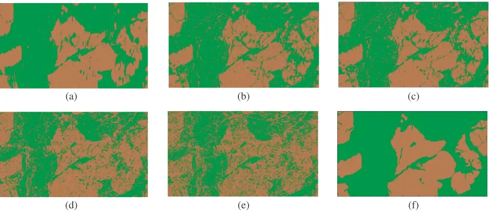
Figure 10 shows the classified images in ROI 1 with different methods. It is observed that the output image of CNN, in Fig. 10(a), displays fewer speckles than those of the other methods. It was mentioned in [59] that the CNN schematic in Fig. 9 tends to produce smooth spatial distribution of output labels, as compared to other CNN schematics. Label smoothing technique like Markov random field [64] can be applied to remove speckles in Figs. 10(b)–10(e).

Figure 11 shows the classified images of NN, with input vectors of Eqs. (2), (4) and (5), respectively. The classified images with FCM andk-means are similar to those with NN, hence are not shown. When the GLCM feature is not used, Figs. 11(b) and 11(c) show that the boundary of large ice floe is easily recognized, but speckles appear everywhere.

(12)

(a) (b) (c)

(d) (e) (f)

Figure 10. Classiﬁed images of (a) CNN, (b) NN, (c) SVM, (d) FCM and (e)k-means. (f) is reference ground-truth, green: FYI, brown: MYI, winter phase, with input vector of (2).

(a) (b) (c)

Figure 11. Classiﬁed images of NN with (a) input vector of (2), (b) input vector of (4) and (c) input vector of (5).

only, without open water, as listed in Table 1, and both polarimetry entropy H and co-polarization ratioσvv/σhh are not useful in separating MYI and FYI.

When input vector of Eq. (4) is used in FCM and k-means, the two cluster centers fall almost on each other at the end of iterations, suggesting that the input vector of Eq. (4) is not suitable for MYI/FYI classiﬁcation with FCM or k-means. The dash marks in some entries of Table 3 indicate no results.

In general, supervised methods perform better than unsupervised ones. The performance of FCM is similar to that of k-means. The FCM can separate MYI and deformed FYI more accurately than

k-means does because the former has the ﬂexibility to assign a pixel to diﬀerent clusters. Among the supervised methods, CNN outperforms NN and SVM in accuracy rate, with the same input vector.

The accuracy rates of NN, SVM, FCM, and k-means, with input vector of (2), are about 10% higher than their counterparts with input vectors of Eqs. (4) and (5). This implies that GLCM feature

f2 is useful in separating FYI and MYI, possibly because the contrast feature f2 has relatively higher

value on highly deformed FYI than MYI and plain FYI. Including texture feature in the input vector improves the accuracy rate for all the classiﬁcation methods studied in this work, consistent with other sea-ice classiﬁcation studies [8, 22].

(13)

Table 3. Classiﬁcation results in ROI 1 (winter).

[κ1, κ2, f2]t

CNN NN SVM FCM k-means

ground-truth

MYI FYI MYI FYI MYI FYI MYI FYI MYI FYI

predicted MYI 39.0 3.7 36.0 7.4 37.9 9.6 37.0 14.8 33.0 20.5 FYI 2.6 54.7 5.6 51.0 3.8 48.7 4.6 43.6 8.6 37.9

accuracy rate (%) 93.7 87.0 86.6 80.6 70.9

[κ1, κ2]t

ground-truth

accuracy rate (%) 92.5 76.6 75.9 73.7 70.6

¯

C or ¯C¯

ground-truth

predicted MYI 38.9 3.9 29.7 16.3 29.5 18.9 − − − − FYI 2.8 54.4 11.9 42.1 12.2 39.4 − − − −

accuracy rate (%) 93.3 71.8 68.9 − −

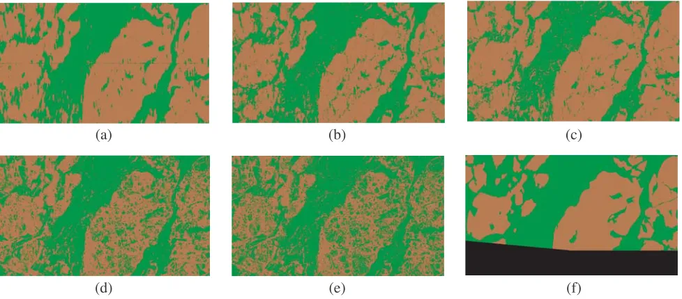
Figure 12 and Table 4 show the classiﬁcation results of ROI 2 in Fig. 2(b). Part of Fig. 12(f) is labeled unknown because no co-located C-band image is available in that part, and using only L-band image of σvv is not eﬀective to classify sea-ice type [7]. The image of ROI 2 in Fig. 2(b) is used to test the

(a) (b) (c)

(d) (e) (f)

(14)

Table 4. Classiﬁcation results in ROI 2 (winter).

[κ1, κ2, f2]t

ground-truth

accuracy rate (%) 86.6 84.6 82.9 77.6 71.9

[κ1, κ2]t

ground-truth

accuracy rate (%) 86.0 75.1 72.8 71.4 68.5

¯

C or ¯C¯

ground-truth

predicted MYI 48.4 7.1 40.3 16.5 48.8 29.2 − − − −

FYI 3.1 41.4 11.1 32.1 2.7 19.3 − − − −

accuracy rate (%) 89.8 72.4 68.1 − −

classiﬁers trained with the image of ROI 1 in Fig. 2(a). It is observed that the accuracy rate in an entry of Table 4 is a little lower than its counterpart in Table 3, because the testing ROI is diﬀerent from the training ROI in the former.

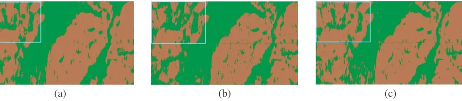
It is observed that the accuracy rate of CNN with input vector of Eq. (4) is 3% higher than those with Eqs. (2) and (5). Also notice the diﬀerence among these classiﬁed images within the blue boxes in Figs. 13(a), 13(b) and 13(c). Some information is lost when using input vectors of Eqs. (2) and (5). The GLCM feature f2 does not improve the performance of CNN as the accuracy rates with input vectors

of Eqs. (2) and (5) are similar. By recapitulating the results shown in Fig. 10, we conjecture that the higher accuracy rate in ROI 1 is due to overﬁt rather than the contribution of GLCM feature f2.

(a) (b) (c)

Figure 13. Classiﬁed images of CNN with (a) input vector of (2), (b) input vector of (4) and (c) input vector of (5).

(15)

(a) (b) (c)

(d) (e) (f)

Figure 14. Classiﬁed images of (a) CNN, (b) NN, (c) SVM, (d) FCM and (e)k-means. (f) is reference ground-truth, supervised classiﬁers trained in ROI 3 and tested in ROI 3, green: FYI, yellow: open water, advanced-melt phase, with input vector of (3).

Table 5. Classiﬁcation results in ROI 3 (advanced-melt).

[κ1, κ2, f2]t

ground-truth

OW FYI OW FYI OW FYI OW FYI OW FYI

predicted OW 12.1 1.3 10.1 3.1 9.9 2.9 14.3 27.1 12.5 23.9 FYI 2.9 83.7 4.7 82.1 4.8 82.2 0.8 57.8 2.6 61.0

accuracy rate (%) 95.8 92.2 91.9 72.1 73.5

[κ1, κ2, f2, H, σvv/σhh]t

ground-truth

predicted OW 14.1 0.6 12.9 1.2 12.8 1.2 14.9 15.7 14.6 35.8 FYI 1.0 84.3 1.9 84.0 2.0 84.0 0.2 69.2 0.5 49.1

accuracy rate (%) 98.4 96.9 96.8 84.1 63.7

¯

C or ¯C¯

ground-truth

predicted OW 13.9 0.6 12.7 1.9 7.5 1.8 1.1 3.0 3.0 0.8 FYI 1.2 84.3 2.1 83.3 7.6 83.1 13.9 81.9 12.0 84.2

accuracy rate (%) 98.2 96.0 90.6 83.0 87.2

(16)

counterparts with the input vector of Eq. (2).

The accuracy rate by using k-means method with the input vector of Eq. (3) is 10% lower than that with the input vector of Eq. (2). When a reduced version of Eq. (3), [f2, H, σvv/σhh]t, is input to

k-means, the accuracy rate remains close to that with Eq. (3). Note that k-means classiﬁes 12/15 of OW to FYI, as listed in Table 5.

Figure 15 shows the classified images in ROI 3 by using the input vector of Eq. (4). Recapitulate that two obvious clusters are observed in Fig. 5(a), corresponding to water and FYI, respectively. However, the classified images in Figs. 15(a), 15(b) and 15(d) by using k-means and FCM with 2 clusters, respectively, do not fully reveal the ground-truth. Fig. 15(a) shows that 95.8% of pixels are classified into FYI. Figs. 15(a) and 15(b) also imply thatk-means delivers different results with different initialization of cluster centers.

(a) (b) (c)

(d) (e) (f)

(g) (h)

Figure 15. Classiﬁed images in ROI 3 by using input vector of (4). (a) k-means with 2 clusters, cluster centers initialized as in [63], (b) k-means with 2 clusters, cluster centers are randomly selected, (c) k-means with 3 clusters, cluster centers initialized as in [63] or randomly selected, (d) FCM with 2 clusters, r = 2, unm randomly initialized, (e) FCM with 3 clusters, r = 2, unm randomly initialized, (f) FCM with 3 clusters, r = 1.1, unm randomly initialized, (g) FCM with 3 clusters, r = 1.1, unm

initialized according to the results of k-means, (h) ground-truth from Fig. 14(f), with high-entropy region marked red.

By further comparison of Figs. 15(a) and 15(b) with Fig. 5(d), we observe that the high-entropy pixels near the right border of ROI 3 belong to minority. Fig. 5(a) is reproduced in Fig. 16, with three clusters enclosed by red curves. The ﬁrst and the second clusters have signiﬁcant PDF, while the third cluster (high-entropy outlier) is less obvious. The high-entropy area in Fig. 5(d) overlaps with the area with lowest backscattering power, as shown in Fig. 4.

(17)

Figure 16. Clusters of (1) water, (2) sea ice and (3) high-entropy outlier.

clusters, the results become sensitive to initialization, as shown in Figs. 15(a) and 15(b). Fig. 15(c) shows the classified image by applyingk-means with randomly initialized cluster centers. The classified image reveal three different labels and is less sensitive to initialization. Fig. 15(e) shows the classified image by applying FCM with three clusters. It is observed that the FCM cannot separate FYI from water because the memberships are close, namely, un0 un1 un2 1/3. Note that k-means can be

viewed as a special case of conventional FCM withunm∈ {0,1} andr = 1 in the objective function.

The FCM withr closer to one implies less fuzziness between clusters, rendering its behavior closer to k-means. The weighting exponent of r = 2 in (7) may be too large when applying FCM with input vector of (4). Figs. 15(f) and 15(g) show the classiﬁed images by using FCM with r = 1.1, where randomly initialized unm is used in Fig. 15(f), and the k-means results are used to initialize unm in Fig. 15(g). Both classiﬁed images look similar to the reference ground-truth shown in Fig. 15(h). The initialization ofunm in Fig. 15(g) is implemented as

unm =

0.6, m=Kn

0.4/(M−1), otherwise

whereKn∈ {0, . . . , M −1} is the classiﬁcation result ofk-means and M is the number of clusters.

By taking a closer look, only two labels are visible in Fig. 15(f) because two of the three cluster centers almost overlap with each other. On the other hand, three labels clearly appear in Fig. 15(g), which implies that proper initialization is important. Table 6 lists the accuracy rates associated with Figs. 15(c), 15(e) and 15(g), respectively.

Table 6. Classiﬁcation results in ROI 3 by using FCM and k-means, with input vector of Eq. (4).

3 clusters, and ¯C¯

k-means FCM, r= 2 FCM, r= 1.1 ground-truth

OW FYI FYI’ OW FYI FYI’ OW FYI FYI’

predicted

OW 3.6 0.6 0.1 0.8 2.1 0.4 11.6 0.2 0.1 FYI 11.5 83.8 0.2 14.3 82.4 0.0 1.0 81.1 0.0 FYI’ 0.0 0.0 0.2 0.0 0.0 0.0 2.6 0.9 0.4

accuracy rate (%) 87.6 83.5 93.4

(18)

7. CONCLUSION

Two unsupervised methods (FCM and k-means) and three supervised methods (SVM, NN and CNN) have been applied to classify sea-ice type (MYI and FYI) and open water by using L-band PolSAR images in winter and advanced-melt phases, respectively. Different input vectors, pending on different scenarios, have also been proposed to increase the accuracy rate. GLCM featuref2has significant effect

on all the methods except the CNN. By applying the NN method to images in the winter phase, using an input vector including GLCM feature f2 results in 87% of accuracy rate, more than 10% higher

than using the other two input vectors. The boundary of MYI appears more clearly, and speckle eﬀect becomes less signiﬁcant by including GLCM feature f2. The CNN method has higher accuracy rate

than the other methods, especially when the covariance matrix is used as the input vector. By including

H and σvv/σhh in the input vector to classify images in the advanced-melt phase, the accuracy rates

with NN, SVM and FCM are increased by 5–12%. By applying the FCM to classify images into three clusters instead of two, with properly tuned weighting exponent and the results of k-means as initial memberships, the accuracy rate is increased to 93.4%.

REFERENCES

1. Lindsay, R. and A. Schweiger, “Arctic sea ice thickness loss determined using subsurface, aircraft, and satellite observations,” Cryosphere, Vol. 9, No. 1, 269–283, 2015.

2. Serreze, M. C. and J. Stroeve, “Arctic sea ice trends, variability and implications for seasonal ice forecasting,” Phil. Trans. R. Soc. A, Vol. 373, No. 2045, 2015.

3. Stroeve, J., M. M. Holland, W. Meier, T. Scambos, and M. Serreze, “Arctic sea ice decline: Faster than forecast,”Geophys. Res. Lett., Vol. 34, No. 9, 2007.

4. Maslanik, J., C. Fowler, J. Stroeve, S. Drobot, J. Zwally, D. Yi, and W. Emery, “A younger, thinner Arctic ice cover: Increased potential for rapid, extensive sea-ice loss,”Geophys. Res. Lett., Vol. 34, No. 24, 2007.

5. Arkett, M., D. Flett, R. De Abreu, P. Clemente-Col´on, J. Woods, and B. Melchior, “Evaluating ALOS-PALSAR for ice monitoring — What can L-band do for the North American ice service?,”

IEEE Int. Geosci. Remote Sensing Symp., Vol. 5, 2008.

6. Howell, S. E. and J. Yackel, “A vessel transit assessment of sea ice variability in the western Arctic, 1969–2002: Implications for ship navigation,”Canadian J. Remote Sensing, Vol. 30, No. 2, 205–215, 2004.

7. Dierking, W. and T. Busche, “Sea ice monitoring by L-band SAR: An assessment based on literature and comparisons of JERS-1 and ERS-1 imagery,” IEEE Trans. Geosci. Remote Sensing, Vol. 44, No. 4, 957–970, 2006.

8. Zakhvatkina, N. Y., V. Y. Alexandrov, O. M. Johannessen, S. Sandven, and I. Y. Frolov, “Classiﬁcation of sea ice types in ENVISAT synthetic aperture radar images,”IEEE Trans. Geosci. Remote Sensing, Vol. 51, No. 5, 2587–2600, 2013.

9. “Canadian ice service digital archive-regional charts: History, accuracy, and caveats,” Rep. 00-02, Ballicater Consulting Ltd, Ottawa, 2006.

10. Onstott, R. G., “Sar and scatterometer signatures of sea ice,”Microwave Remote Sensing Sea Ice, Vol. 68, 73–104, 1992.

11. Drunkwater, M., R. Hosseinmostafa, and P. Gogineni, “C-band backscatter measurements of winter sea-ice in the Weddell Sea, Antarctica,” Int. J. Remote Sensing, Vol. 16, No. 17, 3365–3389, 1995. 12. Geldsetzer, T., J. B. Mead, J. J. Yackel, R. K. Scharien, and S. E. Howell, “Surface-based polarimetric C-band scatterometer for ﬁeld measurements of sea ice,”IEEE Trans. Geosci. Remote Sensing, Vol. 45, No. 11, 3405–3416, 2007.

(19)

14. Barber, D. G., J. Yackel, and J. Hanesiak, “Sea ice, RADARSAT-1 and Arctic climate processes: A review and update,” Canadian J. Remote Sensing, Vol. 27, No. 1, 51–61, 2001.

15. Dammann, D. O., H. Eicken, A. R. Mahoney, E. Saiet, F. J. Meyer, C. John, et al., “Traversing sea ice- Linking surface roughness and ice traﬃcability through SAR polarimetry and interferometry,”

IEEE J. Sel. Topics Appl. Earth Observ. Remote Sensing, Vol. 11, No. 2, 416–433, 2018.

16. Isleifson, D., R. J. Galley, D. G. Barber, J. C. Landy, A. S. Komarov, and L. Shafai, “A study on the C-band polarimetric scattering and physical characteristics of frost ﬂowers on experimental sea ice,”IEEE Trans. Geosci. Remote Sensing, Vol. 52, No. 3, 1787–1798, 2014.

17. Dierking, W., “Mapping of diﬀerent sea ice regimes using images from Sentinel-1 and ALOS synthetic aperture radar,”IEEE Trans. Geosci. Remote Sensing, Vol. 48, No. 3, 1045–1058, 2010. 18. Johansson, A. M., C. Brekke, G. Spreen, and J. A. King, “X-, C-, and L-band SAR signatures of newly formed sea ice in Arctic leads during winter and spring,” Remote Sensing Environment, Vol. 204, 162–180, 2018.

19. Cloude, S. R. and E. Pottier, “A review of target decomposition theorems in radar polarimetry,”

IEEE Trans. Geosci. Remote Sensing, Vol. 34, No. 2, 498–518, 1996.

20. Sandven, S., O. M. Johannessen, M. W. Miles, L. H. Pettersson, and K. Kloster, “Barents Sea seasonal ice zone features and processes from ERS 1 synthetic aperture radar: Seasonal Ice Zone Experiment 1992,” J. Geophys. Res.: Oceans, Vol. 104, No. C7, 1999.

21. Alexandrov, V., S. Sandven, K. Kloster, L. Bobylev, and L. Zaitsev, “Comparison of sea ice signatures in okean and RADARSAT radar images for the northeastern Barents sea,”Canadian J. Remote Sensing, Vol. 30, No. 6, 882–892, 2004.

22. Liu, H., H. Guo, and L. Zhang, “SVM-based sea ice classiﬁcation using textural features and concentration from RADARSAT-2 Dual-Pol ScanSAR data,” IEEE J. Sel. Topics Appl. Earth Observ. Remote Sensing, Vol. 8, No. 4, 1601–1613, 2015.

23. Zhang, Z., H. Wang, F. Xu, and Y.-Q. Jin, “Complex-valued convolutional neural network and its application in polarimetric SAR image classiﬁcation,” IEEE Trans. Geosci. Remote Sensing, Vol. 55, No. 12, 7177–7188, 2017.

24. Zhang, L., W. Ma, and D. Zhang, “Stacked sparse autoencoder in PolSAR data classiﬁcation using local spatial information,” IEEE Geosci. Remote Sensing Lett., Vol. 13, No. 9, 1359–1363, 2016. 25. Lee, J.-S., M. R. Grunes, and R. Kwok, “Classiﬁcation of multi-look polarimetric SAR imagery

based on complex Wishart distribution,”Int. J. Remote Sensing, Vol. 15, No. 11, 2299–2311, 1994. 26. Lee, J.-S., M. R. Grunes, T. L. Ainsworth, L.-J. Du, D. L. Schuler, and S. R. Cloude, “Unsupervised classiﬁcation using polarimetric decomposition and the complex Wishart classiﬁer,” IEEE Trans. Geosci. Remote Sensing, Vol. 37, No. 5, 2249–2258, 1999.

27. Kersten, P. R., J.-S. Lee, and T. L. Ainsworth, “Unsupervised classiﬁcation of polarimetric synthetic aperture radar images using fuzzy clustering and EM clustering,” IEEE Trans. Geosci. Remote Sensing, Vol. 43, No. 3, 519–527, 2005.

28. Fan, J. and J. Wang, “Polarimetric SAR image segmentation based on spatially constrained kernel fuzzy C-means clustering,”IEEE OCEANS, Genova, 2015.

29. Doulgeris, A. P., S. N. Anﬁnsen, and T. Eltoft, “Automated non-gaussian clustering of polarimetric synthetic aperture radar images,”IEEE Trans. Geosci. Remote Sensing, Vol. 49, No. 10, 3665–3676, 2011.

30. Soh, L.-K. and C. Tsatsoulis, “Texture analysis of SAR sea ice imagery using gray level co-occurrence matrices,” IEEE Trans. Geosci. Remote Sensing, Vol. 37, No. 2, 780–795, 1999. 31. Singha, S., M. Johansson, N. Hughes, S. M. Hvidegaard, and H. Skourup, “Arctic sea ice

characterization using spaceborne fully polarimetric L-, C-, and X-band SAR with validation by airborne measurements,” IEEE Trans. Geosci. Remote Sensing, Vol. 56, No. 7, 3715–3734, 2018. 32. Zhang, Y.-D. and L. N. Wu, “Crop classiﬁcation by forward neural network with adaptive chaotic

particle swarm optimization,” Sensors, Vol. 11, 4721–4743, 2011, doi:10.3390/s110504721.

(20)

Real-Time Image Proc., Vol. 15, 631–642, 2018.

34. Watts, S., “Radar sea clutter: Recent progress and future challenges,” IEEE Int. Conf. Radar, 2008.

35. Fois, F., P. Hoogeboom, F. Le Chevalier, and A. Stoﬀelen, “Future ocean scatterometry: On the use of cross-polar scattering to observe very high winds,” IEEE Trans. Geosci. Remote Sensing, Vol. 53, No. 9, 5009–5020, 2015.

36. Valenzuela, G. R., “Theories for the interaction of electromagnetic and oceanic waves: A review,”

Boundary-Layer Meteorology, Vol. 13, No. 1–4, 61–85, 1978.

37. Ulaby, F., R. K. Moore, and A. K. Fung, Microwave Remote Sensing: Active and Passive, from Theory to Applications, Vol. 3, Artech House, 1986.

38. Komarov, A. S., J. C. Landy, S. A. Komarov, and D. G. Barber, “Evaluating scattering contributions to C-band radar backscatter from snow-covered ﬁrst-year sea ice at the winter-spring transition through measurement and modeling,” IEEE Trans. Geosci. Remote Sensing, Vol. 55, No. 10, 5702–5718, 2017.

39. Livingstone, C. E., K. P. Singh, and A. L. Gray, “Seasonal and regional variations of active/passive microwave signatures of sea ice,”IEEE Trans. Geosci. Remote Sensing, No. 2, 159–173, 1987. 40. http://iceweb1.cis.ec.gc.ca/Archive/?lang=en.

41. https://earth.esa.int/web/guest/data-access. 42. https://www.asf.alaska.edu.

43. http://www.eorc.jaxa.jp/ALOS/en/about/palsar.htm.

44. https://directory.eoportal.org/web/eoportal/satellite-missions/e/ers1.

45. Meadows, P., D. Esteban, and P. Mancini, “The ERS SAR performances: An update,”Euro. Space Agency, Vol. 450, 79–84, 2000.

46. Lee, J.-S. and E. Pottier, Polarimetric Radar Imaging: From Basics to Applications, CRC Press, 2009.

47. Freeman, A. and S. L. Durden, “A three-component scattering model for polarimetric SAR data,”

48. Minchew, B., C. E. Jones, and B. Holt, “Polarimetric analysis of backscatter from the Deepwater Horizon oil spill using L-band synthetic aperture radar,” IEEE Trans. Geosci. Remote Sensing, Vol. 50, No. 10, 3812–3830, 2012.

49. Lang, R., Y. Zhou, C. Utku, and D. Le Vine, “Accurate measurements of the dielectric constant of seawater at L band,”Radio Science, Vol. 51, No. 1, 2–24, 2016.

50. Joughin, I. R., D. P. Winebrenner, and D. B. Percival, “Probability density functions for multilook polarimetric signatures,”IEEE Trans. Geosci. Remote Sensing, Vol. 32, No. 3, 562–574, 1994. 51. Anﬁnsen, S. N. and T. Eltoft, “Application of the matrix-variate Mellin transform to analysis of

polarimetric radar images,”IEEE Trans. Geosci. Remote Sensing, Vol. 49, No. 6, 2281–2295, 2011. 52. Nicolas, J.-M. and S. N. Anﬁnsen, “Introduction to second kind statistics: Application of log-moments and log-cumulants to the analysis of radar image distributions,” Trait. Signal, Vol. 19, No. 3, 139–167, 2002.

53. Tison, C., J.-M. Nicolas, F. Tupin, and H. Maˆıtre, “A new statistical model for Markovian classiﬁcation of urban areas in high-resolution SAR images,”IEEE Trans. Geosci. Remote Sensing, Vol. 42, No. 10, 2046–2057, 2004.

54. Skrunes, S., C. Brekke, and A. P. Doulgeris, “Characterization of low-backscatter ocean features in dual-copolarization SAR using log-cumulants,”IEEE Geosci. Remote Sensing Lett., Vol. 12, No. 4, 836–840, 2015.

55. Derrode, S., G. Mercier, J.-M. Le Caillec, and R. Garello, “Estimation of sea-ice SAR clutter statistics from Pearson’s system of distributions,”IEEE Int. Geosci. Remote Sensing Symp., Vol. 1, 190–192, 2001.

(21)

57. Liu, C., W. Liao, H.-C. Li, K. Fu, and W. Philips, “Unsupervised classiﬁcation of multilook polarimetric sar data using spatially variant Wishart mixture model with double constraints,”

58. Aldenhoff, W., C. Heuzé, and L. E. Eriksson, “Comparison of ice/water classification in Fram strait from C-and L-band SAR imagery,” Ann. Glaciology, Vol. 59, No. 76, 112–123, 2018.

59. Badrinarayanan, V., A. Kendall, and R. Cipolla, “Segnet: A deep convolutional encoder-decoder architecture for image segmentation,” IEEE Trans. Pattern Analysis Machine Intell., Vol. 39, No. 12, 2481–2495, 2017.

60. Hsu, C.-W., C.-C. Chang, C.-J. Lin, et al., “A practical guide to support vector classiﬁcation,” https://www.csie.ntu.edu.tw/cjlin/papers/guide/guide.pdf, 2003.

61. Zheng, Y., B. Jeon, D. Xu, Q. Wu, and H. Zhang, “Image segmentation by generalized hierarchical fuzzy c-means algorithm,” J. Intell. Fuzzy Syst., Vol. 28, No. 2, 961–973, 2015.

62. Dabboor, M., J. Yackel, M. Hossain, and A. Braun, “Comparing matrix distance measures for unsupervised PolSAR data classiﬁcation of sea ice based on agglomerative clustering,” Int. J. Remote Sensing, Vol. 34, No. 4, 1492–1505, 2013.

63. Arthur, D. and S. Vassilvitskii, “k-means++: The advantages of careful seeding,” Annual ACM-SIAM Symp. Discrete Algorithms, 1027–1035, 2007.

64. Zhang, Y., M. Brady, and S. Smith, “Segmentation of brain MR images through a hidden Markov random ﬁeld model and the expectation-maximization algorithm,” IEEE Trans. Med. Imag., Vol. 20, No. 1, 45–57, 2001.