Implementing 4-Dimensional GLV Method on
GLS Elliptic Curves with
j
-Invariant 0
Zhi Hu1, Patrick Longa2?, and Maozhi Xu1
1 School of Mathematical Sciences,
Peking University, Beijing,100871, P.R.China
{huzhi,mzxu}@math.pku.edu.cn
2 Microsoft Research,
One Microsoft Way, Redmond, WA 98052, USA [email protected]
Abstract. The Gallant-Lambert-Vanstone (GLV) method is a very ef-cient technique for accelerating point multiplication on elliptic curves with eciently computable endomorphisms. Galbraith, Lin and Scott (J. Cryptol. 24(3), 446-469 (2011)) showed that point multiplication exploit-ing the2-dimensional GLV method on a large class of curves over Fp2
was faster than the standard method on general elliptic curves overFp,
and left as an open problem to study the case of4-dimensional GLV on
special curves (e.g.,j(E) = 0) over Fp2. We study the above problem
in this paper. We show how to get the4-dimensional GLV
decomposi-tion with proper decomposed coecients, and thus reduce the number of doublings for point multiplication on these curves to only a quarter. The resulting implementation shows that the4-dimensional GLV method
on a GLS curve runs in about0.78the time of the2-dimensional GLV
method on the same curve and in between0.78-0.87the time of the2
-dimensional GLV method using the standard method overFp. In
partic-ular, our implementation reduces by up to27%the time of the previously
fastest implementation of point multiplication on x86-64 processors due to Longa and Gebotys (CHES2010).
Key words: Elliptic curves, point multiplication, GLV method, GLS curves.
1 Introduction
The fundamental operation in elliptic curve cryptography is point multiplication. In 2001, Gallant, Lambert, and Vanstone [10] described a new method (a.k.a. GLV method) for accelerating point multiplication on certain classes of elliptic curves with eciently computable endomorphisms. Let E be an elliptic curve over a nite eldFq and letP ∈E(Fq)have prime orderr. Given an eciently computable endomorphism ψ for E s.t. ψ(P) = [λ]P ∈ hPi, the GLV method
?This work was partially carried out while the author was at the University of
consists in replacing the computation[k]P by a multi-scalar multiplication with the form[k1]P+ [k2]ψ(P), where the decomposition coecients|k1|,|k2| ≈r1/2. Since the number of doublings is halved, this method potentially injects a signif-icant speedup in the point multiplication computation on these elliptic curves. This approach might be generalized to m-dimensional case, which can achieve further speedups, if one could get higher degree decompositions with the form
[k1]P+ [k2]ψ(P) +. . .+ [km]ψ(P)m−1 where|ki| ≈r1/m.
Constructing eciently computable endomorphisms is one of the key prob-lems in the GLV method. Gallant, Lambert and Vanstone gave some special examples in [10]. In 2002, Iijima, Matsuo, Chao and Tsujii [15] constructed an ecient computable homomorphism on elliptic curves E(Fp2) with j(E) ∈ Fp arising from the Frobenius map on a twist ofE. Galbraith, Lin, and Scott [7,8] generalized their construction for a large class of elliptic curves overFp2 (referred
to as GLS curves) and applied the GLV method. They gave detailed implemen-tations on these curves, showing that their method ran in between0.70and0.84
the time of the best methods for elliptic curve point multiplication on general curves at that time. A detailed analysis on various x86-64 processors was carried out in [20] and later extended by Longa in [18]. Longa showed that GLS curves over Fp2 reduce costs in the range 9%-45% in comparison with general curves
over Fp, implying that the boost in performance obtained with GLS tightly
depends on the particular platform.
Since previous applications of the GLV method have been limited to dimen-sion 2, scalar decomposition with coecients of size O(r1/2) has been exten-sively studied [17,23,25,9,7,8]. In an earlier work [27], Zhou et al. tried the LLL algorithm [6, Alg. 2.6.3] to get a reduced basis for computing Babai rounding in the 3-dimensional case. Galbraith, Lin and Scott also showed how to get a 4-dimensional construction on certain GLS curves with j-invariant 0. Simulta-neously to the present work, Birkner and Sica [4] have proposed a 4-dimensional decomposition method and provided a general bound for the size of the coe-cients given byO(C·r1/4)for some explicitC >100.
Our contributions can be summarized as follows:
We describe an explicit lattice basis with good properties for4-dimensional
GLV decomposition on GLS curves withj-invariant 0. The decomposed coef-cients are shown to have sizeO(2√2r1/4)≤2√2p, thus enable the reduction of the number of doublings on these curves to a quarter.
We extend Brown, Myers and Solinas's decomposition method for compact curves to support 2-dimensional GLV decomposition on ordinary curves
with j-invariant 0 [5]. According to Sica et al.'s analysis [25], our upper bound for the size of decomposition coecients is optimal.
We realize high-speed implementations of point multiplication at the 128-bit security level on x86-64 processors usingj-invariant 0 curves: i) overFpusing the2-dimensional GLV method; ii) over Fp2 using the 2-dimensional GLV
method; and iii) overFp2 using the4-dimensional GLV method.
The resulting implementations show that the4-dimensional GLV method on
on the same curve and in between0.78-0.87the time of the 2-dimensional GLV
method using the standard method overFp. In comparison with the previously
fastest implementation due to Longa and Gebotys [20] (see also [18, Ch. 5]), which uses a2-dimensional GLV-based GLS curve with Twisted Edwards
coor-dinates and runs in 166,000 cycles on a 2.7GHz Intel Core i7-2620M processor, the presented GLV4-based implementation reduces the time by up to27%,
run-ning in only 122,000 cycles on the same platform. It is also much faster than the very recent implementation by Bernstein, Duif, Lange, Schwabe and Yang [2], which runs in 194,000 cycles on the same platform (i.e., our result reduces their time by37%in this case).
The rest of the paper is organized as follows. Section 2 presents the nition of twist maps on elliptic curves and their constructions. Section 3 de-scribes Galbraith-Lin-Scott elliptic curves and some eciently computable en-domorphisms on them. In Section 4 we describe our decomposition method for supporting 4-dimensional GLV. In Section 5 we present a 2-dimensional GLV
decomposition method for ordinary curves over Fp with j-invariant 0. Our ef-cient implementations and the corresponding benchmark results are described in Section 6. We end this paper with some conclusions in Section 7.
2 Twists on Elliptic Curves
LetEandE0 be two elliptic curves over
Fq whereqis a power of some primep. E0 is called a twist of degreedofE if there exists an isomorphismφd:E0→E dened over Fqd and d is minimal. If E0 is a degree d twist of E, then the
automorphism groupAut(E)must contain an element of orderd[12]. Moreover, ifp≥5, we have#Aut(E)|6according to [26, Th. III.10.1].
All twists can be described explicitly as in [26, Prop. X.5.4]. Supposep≥5,
the set of twists of E is canonically isomorphic to Fq∗/(Fq∗) d
with d = 2 if
j(E)6= 0,1728, d= 4ifj(E) = 1728and d= 6ifj(E) = 0. LetE be given by a short Weierstrass equation y2=x3+ax+b witha, b∈
Fq andD ∈F∗q. The twists corresponding toDmod (F∗q)d are given by
d= 2 :y2=x3+a/D2x+b/D3,
φd:E0→E: (x, y)7→(Dx, D3/2y) d= 4 :y2=x3+a/Dx,
φd:E0→E: (x, y)7→(D1/2x, D3/4y) d= 6 :y2=x3+b/D,
φd:E0→E: (x, y)7→(D1/3x, D1/2y).
Iijima, Matsuo, Chao and Tsujii [15] constructed an ecient computable homomorphism on elliptic curvesE(Fpk) arising from the Frobenius map πon
a twist ofE:
ψd:E0(Fpk)
φd
→E(Fpdk)
π
→E(Fpdk)
φ−1 d
3 The GLS Elliptic Curves
Galbraith, Lin and Scott [7,8] implemented the 2-dimensional GLV method by
using an eciently computable homomorphism on elliptic curves overFp2. They
generalized Iijima et al.'s construction as follows:
Theorem 1. [7,8] LetEbe an elliptic curve dened overFq such that#E(Fq) = q+ 1−t and letφ:E→E0 be a separable isogeny of degreei dened over Fqk
where E0 is an elliptic curve dened over Fqm with m|k. Let r|#E0(Fqm) be a
prime such that r > i and r|#E0(Fqk). Let π be the q-power Frobenius map
on E and let φˆ : E0 → E be the dual isogeny of φ. Dene ψ = φπφˆ, then ψ ∈ EndF
qk(E
0), and for P ∈ E0(
Fqk) we have ψk(P)−[ik]P = OE0 and ψ2(P)−[it]ψ(P) + [i2q]P =O
E0.
Corollary 1. [7,8] Let p >3 be a prime. Letu be a non-square inFp2. Dene
a0 = u2a and b0 = u3b, then E0(Fp2) : y2 = x3+a0x+b0 is the quadratic
twist of E(Fp2) and#E0(Fp2) = (p−1)2+t2. Deneφ(x, y) = (ux, u3/2y)and
ψ=φ−1πφ. ForP ∈E0(
Fq2)[r], we haveψ(P)2+P =OE0, and ψ(P) = [λ]P whereλ≡t−1(p−1) modr.
Consider the latticeL={(x, y)∈Z2 :x+yλ≡0 modr}. Galbraith et al.
used the basis{(t, p−1),(1−p, t)}of some latticeL0⊂Lto get the2-dimensional
decomposition, with each coecient bounded by(p+ 1)/√2.
Galbraith et al. also described how to get higher dimensional expansions by using elliptic curvesEoverFp2 with#Aut(E)>2. The basic principle is to use
a twist φ:E→E0 whereE0 is dened overFp2 andφis dened overFp2d, and
not dened over any subeld of Fp2d, for some even integer d ≥ 4. A natural
example is to use twist of degree 6 on elliptic curves withj-invariant 0.
Corollary 2. [7,8] Let p≡1 mod 6 and let B ∈F∗p. Dene E :y2 =x3+B.
Chooseu∈F∗p12 such thatu6∈Fp2 and deneE0:y2=x3+u6B overFp2. The
isomorphism φ : E0 → E is given by φ(x, y) = (u2x, u3y) and is dened over
Fp12. Let ψ=φ−1πφ. For P ∈E0(Fp2), we have ψ4(P)−ψ2(P) +P =OE0. Hence the 4-dimensional GLV method can be eciently applied to these
curves. Note that−ψ2 satises the characteristic equation x2+x+ 1 = 0 and so acts as the standard automorphism (x, y)7→(ζ3x, y)on E0; ψ3 satises the characteristic equationx2+ 1 = 0and so acts as the homomorphism in Corollary 1.
4 4-Dimensional GLV Method on GLS Curves with
j
-Invariant 0
Let E0, ψ be dened as in Corollary 2, and suppose r|#E0(Fp2) is prime. We
following we show how to decompose the scalarkin suitable coecients of size O(r1/4).
Let P ∈ E0(Fp2) be a point of order r, and suppose ψ(P) = [λ]P where λ ∈ Z/rZ. Denote h·,·i as the inner product of two vectors. Dene vectors
Ψ = (1, ψ, ψ2, ψ3), Λ = (1, λ, λ2, λ3), and lattice L = {(k
0, k1, k2, k3) ∈ Z4 :
h(k0, k1, k2, k3),Λi ≡ 0 modr}. Let {v0,v1,v2,v3} be a basis for lattice L0,
where 0⊂L0 ⊆L. By Babai rounding method, we can decompose the scalark ask≡ h(k0, k1, k2, k3),Λimodr, wheremaxi{|ki|} ≤2 maxi{kvik}.
In order to nd a proper lattice basis{v0,v1,v2,v3}that satises the upper
bound maxi{kvik} = O(r1/4), we rst study the relations among the
charac-teristic p, the group order r and the Frobenius trace t on our targeted elliptic curves.
Lemma 1. Letnbe an integer, then the binary quadratic formx2+xy+y2=n has 6M(n) integral solutions, whereM(n) = #{k :k|n, k ≡1 mod 3} −#{k :
k|n, k≡2 mod 3}.
Proof. Since the discriminant of the binary quadratic form is−3and the number
of classes h(−3) = 1, from Theorem 1 in [14, Ch. 12.4] we can obtain that the
number of integral solutions is6Σk|n(−k3), where(·)is the Kronecker symbol. It follows that 6Σk|n(−k3) = 6M(n)by the denition of Kronecker symbol. ut
Lemma 2. Let pbe prime. If the equation x2+xy+y2 = phas one integral solution, then there exist exactly12integral solutions.
Proof. Let T = {(x, y) ∈Z2 : x2+xy+y2 =p}. If (a, b) ∈ T, then T is not
an empty set, which implies thatp≡1 mod 3. By Lemma 1,#T = 12. We can
easily verify that
T0 ={(a, b),(−a,−b),(b, a),(−b,−a),
(a+b,−a),(−a−b, a),(−a, a+b),(a,−a−b),
(a+b,−b),(−a−b, b),(−b, a+b),(b,−a−b)}
is also a set of solutions forx2+xy+y2 =p. Since pis prime, we must have gcd(a, b) = 1. Then the vectors inT0 are pairwise dierent, and thusT =T0. ut
For counting the rational points on our targeted curves, we have the next theorem.
Theorem 2. [16, Ch. 18.3,Th. 4] Let p≥5 be prime and p-B. Consider the elliptic curve E:y2=x3+B over
Fp. If p≡2 mod 3then#E(Fp) =p+ 1. If p≡1 mod 3letp=ππ withπ∈Z[ω] andπ≡2 mod 3. Then
#E(Fp) =p+ 1 + (
4B π )6
π+ (4B
If p≡ 1 mod 3, by the construction in Lemma 2, we can nd one integral
solution (a, b) ∈ T such that a ≡ 2 mod 3, b ≡ 0 mod 3. So we can choose
π=a−bωin Theorem 2, and thenp=ππ=a2+ab+b2. Hence there are six cases of Frobenius tracet=−(4Bπ )6π−(4Bπ )6πgiven by
t=±(a+ 2b),±(2a+b),±(a−b).
#E0(Fp2) can be computed through [12, Prop. 8]. For example, if t = p+ 1−#E(Fp) =a+ 2b, we can obtain that#E0(Fp2) = (p−1)2+ (2a+b)2 or
#E0(Fp2) = (p−1)2+ (a−b)2. In fact, if we assume that #E0(Fp2)is prime or
nearly prime, there are only three cases of#E0(Fp2)given by
r1(a, b) = (p−1)2+ (a+ 2b)2, r2(a, b) = (p−1)2+ (2a+b)2, r3(a, b) = (p−1)2+ (a−b)2.
By Theorem 1 we haveψ4−ψ2+ 1 = 0andψ2−tψ+p= 0, and the following proposition can be dened.
Proposition 1. Let notation be as above. Suppose thatp=a2+ab+b2, where a, b∈Z, a≡2 mod 3, b≡0 mod 3. For
(1)#E0(Fp2) =r1(a, b), dene λ0≡a(1−p)(b2+ 2ab+ 1)−1modr; (2)#E0(Fp2) =r2(a, b), dene λ0≡b(1−p)(a2+ 2ab+ 1)−1modr;
(3)#E0(Fp2) =r3(a, b), dene λ0 ≡(bp−a)(b2+ 2ab−1)−1modr.
Then λ0 satises λ04−λ02+ 1 ≡ 0 modr. Moreover, there exists some i ∈
(Z/12Z)∗ such that ψi(P) = [λ0]P.
Proof. We only give the detailed proof for case (1), the other two cases are analogous. Letx=a(1−p), y=b2+2ab+1, f =x4−x2y2+y4. Sincer|#E0(
Fp2), gcd(y, r) = 1and
f =r1(a, b)·(a8+ 2a7b+ 3a6b2−3a6+ 2a5b3−6a5b+a4b4+ 2a4 −10a4b2−4a3b3+ 2a3b−a2b4+ 11a2b2+ 6ab3+ 6ab+b4+ 2b2+ 1).
We obtain that λ0 ≡ y−1x(modr) satises λ04
−λ02+ 1≡ 0 modr. Moreover, sinceψ4(P)−ψ2(P) +P =OE0, there must exist some i∈(Z/12Z)∗ such that
ψi(P) = [λ0]P. ut
For convenience, we assume thatλ=λ0 in the following. Otherwise we can replaceψwith some ψi, wherei∈(Z/12Z)∗.
Proposition 2. Let notation be as above. For (1)#E0(
Fp2) =r1(a, b), dene v= (1,−a,0,−b);
(2)#E0(
Fp2) =r2(a, b), dene v= (1,−b,0,−a);
(3)#E0(Fp2) =r3(a, b), dene v= (1,−a−b,0, a).
Proof. We only give proof for case (1); the other two cases are analogous. Let x, ybe dened as in Proposition 1. Since
y3hv,Λi=r1(a, b)·(a5b+a4b2−2a3b+a3b3+a2b2+ 4ab+b2+ 1),
it follows that hv,Λi ≡0 modr. ut
Proposition 3. Let notation be as above. Dene the matrix
A=
0 1 0 0 0 0 1 0 0 0 0 1
−1 0 1 0
,
and vectorsvi=vAi,i= 0, . . . ,3. Then{v0,v1,v2,v3} is a basis for a
sublat-tice of L.
Proof. We only give proof for the case#E0(Fp2) =r1(a, b); the other two cases
are analogous. Because hvi,Λi= 0, we havevi∈L. Sincedet(v0,v1,v2,v3)6= 0, we dene latticeL0=v0Z+v1Z+v2Z+v3Z, and thenL0 ⊆L. ut
Note that det(v0,v1,v2,v3) = #E0(Fp2), thus L0 is a sublattice of Z4 of
indexr1(a, b). Ifr= #E0(Fp2), we haveL0 =L.
Theorem 3. For any integerk∈[1, r),{v0,v1,v2,v3}induces a4-dimensional
GLV decompositionk≡k0+k1λ+k2λ2+k3λ3modr, withmaxi{|ki|} ≤2 √
2p=
O(2√2r1/4).
Proof. We only give proof for the case#E0(Fp2) =r1(a, b); the other two cases
are analogous. By Proposition 3, we have
v0=v= (1,−a,0,−b),v1=vA= (b,1,−a−b,0),
v2=vA2= (0, b,1,−a−b),v3=vA3= (a+b,0,−a,1).
Since|a−b| ≥1, we have that|ab| ≤(a2+b2−1)/2 and
p=a2+b2+ab≥a2+b2−(a2+b2−1)/2 =kv0k
2 /2.
Thuskv0k ≤
√
2p.
Note that(−a,−b),(b,−a−b),(a+b,−a)all satisfy the quadratic formx2+ xy+y2=pby Lemma 2. We havekvik ≤
√
2p,i= 0, ...,3. Thus
max
i {|ki|} ≤2 maxi {kvik} ≤2
p
2p=O(2√2r1/4).
u t
Remark 1. The 4 dimensional decomposition for GLS curves withj-invariant
1728can be done in a similar way. In this case we nd that the integral solutions
5 2-Dimensional GLV Method on Ordinary Curves with
j
-Invariant 0
For comparison, we also consider ordinary elliptic curves overFpwithj-invariant 0. Letp≡1 mod 3be prime andE(Fp) :y2=x3+Bbe such an ordinary elliptic curve. Also, let r|#E(Fp)andr >2
p
#E(Fp)be prime.
There is a standard automorphism ψ(x, y) = (ζ3x, y) = [λ](x, y) on this elliptic curve. ForP ∈E(Fp),ψ2(P)+ψ(P)+P =OE. Thusλ2+λ+1≡0 modr, which implies thatr≡1 mod 3.
Two-dimensional GLV decomposition methods for this case have been pro-posed in [17,23,25]. Here we extend Brown, Myers and Solinas's decomposition method for compact curves to decompose the scalar. They regarded ψas the third root of unity ω = (−1 +√−3)/2 ∈ C, and considered decomposing k in the algebraic integer ringZ[ω].
TheRoundoperation dened in [5] as
Round[s+zω] :=b(bs+zc+b2s−zc+ 2)/3c
+b(bs+zc+b2z−sc+ 2)/3c ·ω,
rounds an element s+zω∈Q[ω] to the closest element ofZ[ω] with Euclidean
distance≤1/√3, which, essentially, is a tool to solve the closest vector problem
in some lattice ofZ[ω].
Lemma 3. Let notation be as above. If there exist a, b∈Zsuch that a2+ab+
b2=r, then forP ∈E(Fp)[r], either (a−bψ)(P) =OE or(b−aψ)(P) =OE.
Proof. It easily follows sincea−bλ≡0 modrorb−aλ≡0 modr.
Since r ≡ 1 mod 3, by Cornacchia algorithm [6, Alg. 1.5.3] we can get an
integral solution(x, y)to the equationx2+ 3y2= 4rsuch thata= (x+y)/2and
b=−y(a, b∈Z)satisfya2+ab+b2=r. In practice, we usually choose elliptic
curves generated by the complex multiplication method such that #E(Fp) =r. In the parameter generation stage we have4p= 3s2+t2 for somes, t∈
Z. Then
we obtain a= (t+s−2)/2andb=−s, which satisfya2+ab+b2=r.
By Lemma 3 and the property of theRoundoperation, we obtain the next
result.
Theorem 4. Let notation be as above and P ∈E(Fp)[r]. If(a−bψ)(P) =OE andk−(a−bω)Round[k/(a−bω)] =k1+k2ω, then[k]P= [k1]P+ [k2]ψ(P), wheremax{|k1|,|k2|} ≤2
√ r/3.
6 Performance Evaluation
In this section, we evaluate the performance of dierent variants of the GLV method in practice. The main objective is to determine the gain obtained with the use of GLS curves with j-invariant 0 exploiting the 4-dimensional GLV method. We describe an ecient parameter selection, carry out the correspond-ing operation count and present timcorrespond-ings when computcorrespond-ing a variable-scalar vari-able-point scalar multiplication at the 128-bit security level on representative x86-64 processors. We compare results of four ecient alternatives based on: a GLS curve with j-invariant 0 using 4-dimensional GLV; a GLS curve with j-invariant 0 using 2-dimensional GLV; a GLS curve with Twisted Edwards co-ordinates using 2-dimensional GLV; and an ordinary j-invariant 0 curve using 2-dimensional GLV.
6.1 Curves
GLS curve with j-invariant 0 using 4-dimensional GLV. In this case, we use the elliptic curve given by the equation
E10 :y2=x3+u·7 (1)
dened overFp2
1, wherep1 = 2
128−40557,u∈
Fp2
1 and #E
0
1(Fp2
1) = 0xFFFFF
FFFFFFFFFFFFFFFFFFFFFFEC327FF5BF96F8A8A7FFFE37C5E4F5FA9A 8CD is a 256-bit prime. We have that p1 =a2+ab+b2, a=−5328132332142
06943 and b = 18707378648059847118, where a≡2 mod 3, b ≡0 mod 3. Note
that p1 ≡3 mod 8 and hence Fp2
1 =Fp1[i], where i
2 =−1. Let u= 1 +i and ξ = 45401944847829159044964786890828045383 (ξ3 ≡ 1 modp1). The homo-morphism on ane points of E01is given by
ψ(x, y) = (w2xp, w3yp) = [λ](x, y), where
w=ξ2u(1−p)/6= 274247897208633065225091197380782857056 + 2742478972 08633065225091197380782857056i,
λ=a(1−p)(b2+ 2ab+ 1)−1modr
= 426408418061806223086189537530769555908320353659075508641649191
26143300965390.
The4-dimensional GLV decomposition is described in Section 4.
GLS curve with j-invariant 0 using 2-dimensional GLV. In this case, we also use curve equation (1) dened overFp2
1 withψ1=ψ
GLS curve with Twisted Edwards coordinates using 2-dimensional GLV. For this case, we use the elliptic curve given by the equation
E20 :−ux 2
+y2= 1 + 109ux2y2 (2)
dened overFp2
2 with the Mersenne primep2= 2
127−1;u= 2 +i∈
Fp2 2 is
non-square. Also,#E20(Fp2) =0xFFFFFFFFFFFFFFFFFFFFFFFFFFFFFFFA626
1414C0DC87D3CE9B68E3B09E01A5= 4r, whereris a 252-bit prime. Note that the same curve is used in [20].
Ordinary curve with j-invariant 0 using 2-dimensional GLV. For this case, we use the elliptic curve given by the equation
E3:y2=x3+ 5 (3)
dened over Fp3 with the pseudo-Mersenne prime p3 = 2
256 −1539. Also,
#E3(Fp3) =0xFFFFFFFFFFFFFFFFFFFFFFFFFFFFFFFEF95AE576CE7C
6CCA38E2B32E6FB6214B, which is a 256-bit prime. The 2-dimensional GLV
decomposition method is described in Section 5.
6.2 Operation Count and Timings
For all implementations using the curves above we apply the interleaving method (INT) [11, Alg. 3.51] to perform the multi-scalar multiplication with dimension m, wherem= 2,4. To compute [k]P =P
i[ki]ψ
i(P)where i={0,1, ..., m−1} and P is a variable point, we use the (fractional) width-w non-adjacent form (denoted by (f)wNAF) representation of each ki, where log2|ki| ≈log2|k|/m. In this case we need to precompute Pj = [j]P and [j]ψi(P) = ψi(Pj) for j ={1,3,5, ..., t} andi ={1,2, ..., m−1}. Denote by DBL, mADD and ADD the cost of performing point doubling, mixed addition and addition on a given curve, respectively. Denote by Precomp the cost of precomputingPj= [j]P and
[j]ψi(P) =ψi(P
j). The expected cost of computing[k]P is approximately
log2|k|·(( 2
t+ 1)·δfwNAF·mADD+ (
t−1
t+ 1)·δfwNAF·ADD+ 1
m·DBL) +P recomp,
whereδfwNAF= blog2tc + (t+ 1)/(2blog2tc) + 1−1
.
The costs of mADD, ADD and DBL depend on the chosen coordinate system. In the following, we assume that the costs of multiplication by 2, division by 2 and subtraction are roughly equivalent to addition for simplication purposes. For the case of elliptic curves with j-invariant 0 we use Jacobian coordinates. A state-of-the-art doubling formula can be found in Longa [18, formula (6.7)], which involves 3 multiplications, 4 squarings and 7 additions (note that line eval-uation operations are not considered). Addition formulas are taken from [11]. Point addition involves 11 multiplications, 3 squarings and 7 additions (Z2
Z3
j are precomputed), and mixed addition involves 8 multiplications, 3 squarings and 7 additions. For the case of Twisted Edwards curves we use mixed homoge-neous/extended homogeneous coordinates [13]. Formulas considered in this work can be found in [18, Appendix B1]. Point doubling involves 4 multiplications, 3 squarings and 7 additions; point addition involves 9 multiplications and 9 addi-tions; and mixed addition involves 8 multiplications and 9 additions (considering that the cost of a multiplication with the curve parameteruis approx. equivalent to 2 additions).
Interestingly enough the LM precomputation scheme [21] also applies to curves withj-invariant 0. Since inversion in the quadratic extension eld is not so expensive, we use the scheme that converts precomputation points to ane (cost given by [18, formula (3.6)]) for the GLS curves over Fp2
1. In the case of
the ordinary curve overFp3 precomputed points are left in Jacobian coordinates
(cost given by [18, formula (3.4)]). For the 2- and 4-dimensional GLV method on GLS curves we need to compute 1 and 3 tables with the form[j]ψi(P) =ψi(P
j), respectively. In these cases each multiplication by ψ costs approx. 2 multipli-cations and 1 addition. Since we set t = 13 (optimal), the cost is given by 14
multiplications and 7 additions in the 2-dimensional case and 42 multiplications and 21 additions in the 4-dimensional case. The total cost of Precomp is then 69 multiplications, 17 squarings, 56 additions and 1 inversion for dimension 2 and 97 multiplications, 17 squarings, 70 additions and 1 inversion for dimen-sion 4. For the ordinary curve using 2-dimendimen-sional GLV, the cost of multiplying by ψ is approx. one multiplication. Since in this case t = 15 (optimal), the
cost of computing [j]ψi(P) = ψi(P
j) is given by 8 multiplications. Then the total cost of Precomp is 52 multiplications, 25 squarings and 56 additions. For Twisted Edwards we follow a traditional precomputation scheme (see details in [18, Sec. 5.6.2]). To compute the table[j]ψi(P) =ψi(P
j)witht= 15(optimal) one needs 7 multiplications with ψ on projective points, each costing approx. 4 multiplications, 1 squaring and 1.5 additions; and one multiplication with ψ on an ane point, costing 2 multiplications and 1 addition. Thus the cost is 30 multiplications, 7 squarings and 11.5 additions; and the total cost of Precomp is 97 multiplications, 9 squarings and 80.5 additions.
Finally, at the end of point multiplication the result should be converted to ane. This cost is given by 1 inversion, 3 multiplications and 1 squaring in those cases using Jacobian coordinates; and 1 inversion and 2 multiplications in the case using Twisted Edwards coordinates.
Table 1. Point multiplication operation count, 128-bit security level
Curve Method Operation Count
E01(Fp2
1)128-bitp 4GLV+INT, 7pts. 648.0m+407.5s+829.5a+2i
E01(Fp2
1)128-bitp 2GLV+INT, 7pts. 812.0m+663.5s+1263.5a+2i
E02(Fp22)127-bitp[20,18] 2GLV+INT, 8pts. 994.5m+393.0s+1360.8a+1i
E3(Fp3)256-bitp 2GLV+INT, 8pts. 892.8M+666.1S+1250.9A+1I
As can be seen, extending GLV from two to four dimensions introduces a signicant reduction in the number of operations on thej-invariant 0 GLS curve E1. The GLS curve using 4-dimensional GLV is also signicantly more ecient in0
terms of operation counts than a state-of-the-art implementation based on the GLS-based Twisted Edwards curve E20 using 2-dimensional GLV [20][18]. The comparison with the ordinary curve E3 with j-invariant 0 using 2-dimensional GLV is more complicated. Although quadratic extension eld operations are de-ned on a smaller eld each one requires a few eld operations internally (e.g., a multiplication overFp2 involves 3 eld multiplications and 5 eld additions when
using Karatsuba). Actual implementations are ultimately required to determine eciency.
We have implemented the dierent variants mostly in C language using the MIRACL library [24]. We have written most relevant eld operations in assembly and applied aggressive optimizations at the dierent arithmetic levels closely fol-lowing the techniques discussed in [20][18]. Cycle counts obtained when running the implementations on a 2.80GHz Intel Xeon W3530 (Westmere architecture), a 3.0GHz AMD Phenom II X4 940 (Phenom II architecture) and a 2.7GHz In-tel Core i7-2620M (Sandy Bridge architecture) are detailed in Table 2. In our tests we averaged the cost of105variable-scalar variable-point scalar multiplica-tions and approximated the results to the nearest 1000 cycles. All experiments were performed on one core of the targeted processors using the GNU Compiler Compilation tool (a.k.a. GCC) for compilation.
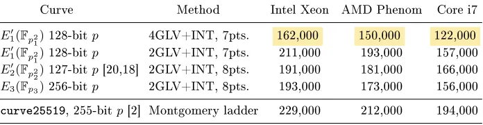
Table 2. Point multiplication timings (in clock cycles), 64-bit processors
Curve Method Intel Xeon AMD Phenom Core i7
E10(Fp2
1)128-bitp 4GLV+INT, 7pts. 162,000 150,000 122,000
E10(Fp2
1)128-bitp 2GLV+INT, 7pts. 211,000 193,000 157,000
E20(Fp2
2)127-bitp[20,18] 2GLV+INT, 8pts. 191,000 181,000 166,000
E3(Fp3)256-bitp 2GLV+INT, 8pts. 193,000 173,000 156,000
Closely following results from the operation count analysis, our GLS-based implementation using 4-dimensional GLV is faster than the state-of-the-art GLS-based implementation using Twisted Edwards with 2-dimensional GLV. In fact, these timings set a new speed record for point multiplication on x86-64 proces-sors. For instance, on an AMD Phenom II X4 940 processor the new implemen-tation reduces the best numbers presented by Longa [18, Ch. 5] in 17%. This translates to a latency of only 50us per point multiplication running on one core and a throughput of 80,000 point multiplications/second running on the four cores of the targeted AMD processor. Moreover, on an Intel Core i7-2620M pro-cessor the same implementation runs in an unprecedented mark of 122,000 cycles, enabling the computation of point multiplication in only 45us (with 2.7GHz as working frequency). The later implies a reduction of 27% in comparison with the 2-dimensional GLV implementation using Twisted Edwards [20,18].
In comparison with an ordinary curve using 2-dimensional GLV, the use of the GLS method for enabling a 4-dimensional GLV injects cost reductions in between 13% and 22%. Our results also show that the use of dimension 2 with GLS-basedj-invariant 0 curves is insucient to get competitive with the standard approach.
In Table 2, we also include cycle counts for the recent implementation of curve25519 by Bernstein et al. [2]. The results were obtained by running their software on exactly the same platforms, with the same compilation tool and un-der the same test conditions (e.g., using only one core with Intel's Turbo Boost and Hyper-Threading disabled). Also note that these results closely follow those available online on eBATS [3] for similar processors (see hydra2 for the case of Intel Xeon, hydra1 for the case of AMD Phenom and sandy0 for the case of Intel Core i7). In general all our implementations are signicantly faster than curve25519 (independently of the method). In particular, our GLV4-based im-plementation runs in 0.63 the time of curve25519 on a Core i7 based on the Sandy Bridge architecture, and on a Westmere machine (i.e., the architecture tar-geted by [2]) our implementation runs in 0.71 the time of curve25519. However, there are important factors that should be noted. On one side, curve25519 is ad-ditionally protected against certain side-channel attacks. On the other hand, our implementations are immediately useful for any elliptic-curve protocol whereas the use of a Montgomery curve limits the applicability of curve25519 to Die-Hellman (DH)-like schemes only.
cycles on the same platforms, respectively. Thus, it can be seen that our 4-GLV implementation runs 1.63 and 1.31 faster in these two cases.
Finally, we remark the importance of comparing results obtained on the same processor to avoid any bias in code performance comparisons.
For extended benchmark results and comparisons on dierent 64-bit plat-forms, the reader is referred to our online database [19].
7 Conclusion
We studied the performance of the4-dimensional GLV method for faster point
multiplication on some GLS curves with j-invariant0. We showed how to get
the 4-dimensional GLV decomposition with suitable coecients bounded by
O(2√2r1/4), thus enabling the reduction in the number of doublings to only a quarter for point multiplication on these curves. Our high-speed implementa-tions showed that the 4-dimensional GLV method using a j-invariant 0 curve over Fp2 runs in about 0.78 the time of the2-dimensional GLV method on the
same curve and in about0.78-0.87the time of the2-dimensional GLV method on
an ordinary curve overFp, enabling the currently fastest computation of elliptic
curve point multiplication at the 128-bit security level in the literature.
8 Acknowledgments
We would like to thank Steven Galbraith and the reviewers for their very useful comments and suggestions. We also thank Diego F. Aranha for carrying out the performance tests on an Intel Core i5-540M processor. The authors Hu and Xu were supported by the Natural Science Foundation of China (Grant No. 10990011) and Open Foundation of the Key Lab for Information Assurance Technology (Grant No. KJ-11-02).
References
1. Avanzi R., Cohen H., Doche C., Frey G., Lange T., Nguyen K., Vercauteren F.: Handbook of Elliptic and Hyperelliptic Cryptography. Chapman and Hall/CRC (2006)
2. Bernstein D.J., Duif N., Lange T., Schwabe P., Yang B.-Y.: High-speed high-security signatures. In: Preneel B., Takagi T. (eds.) CHES 2011, LNCS, vol. 6917. Springer, Heidelberg (2011). Full version: eprint 2011/368, http://eprint.iacr.org/2011/ 368
3. Bernstein D.J., Lange T.: eBATS: ECRYPT Benchmarking of Asymmetric Systems (eBATS), accessed on August 5, 2011. http://bench.cr.yp.to/ebats.html 4. Birkner P., Sica F.: Four-dimensional Gallant-Lambert-Vanstone scalar
multiplica-tion. ArXiv:1106.5149 (2011). http://arxiv.org/abs/1106.5149
6. Cohen H.: A Course in Computational Algebraic Number Theory. Springer, Berlin (1996)
7. Galbraith S.D., Lin X.B., Scott M.: Endomorphisms for faster elliptic curve cryp-tography on a large class of curves. In: Joux A. (ed.) EUROCRYPT 2009, LNCS, vol. 5479, pp. 518-535. Springer, Heidelberg (2009)
8. Galbraith S.D., Lin X.B., Scott M.: Endomorphisms for faster elliptic curve cryp-tography on a Large class of curves. J. Cryptol. 24(3), 446-469 (2011)
9. Galbraith S.D., Scott M.: Exponentiation in pairing friendly groups using homomor-phisms. In: Galbraith, S.D., Paterson, K.G. (eds.) Pairing 2008. LNCS, vol. 5209, pp. 211-224. Springer, Heidelberg (2008)
10. Gallant R.P., Lambert R.J., Vanstone S.A.: Faster point multiplication on elliptic curves with ecient endomorphisms. In: Kilian J.(ed.) CRYPTO 2001, LNCS, vol. 2139, pp.190-200. Springer, Heidelberg (2001)
11. Hankerson D., Menezes A.J.,Vanstone S.: Guide to Elliptic Curve Cryptography. Springer, Heidelberg (2004)
12. Hess F., Smart N., Vercauteren F.: The eta-pairing revisited. IEEE Trans. Inf. Theory. 52(10), 4595-4602 (2006)
13. Hisil H., Wong K., Carter G., Dawson E.: Twisted edwards curves revisited. In: Pieprzyk J. (ed.) ASIACRYPT 2008. LNCS, vol. 5350, pp. 326-343. Springer, Hei-delberg (2008)
14. Hua L.K.: Introduction to Number Theory, translated from the Chinese by Peter Shiu. Springer, Berlin (1982)
15. Iijima T., Matsuo K., Chao J., Tsujii S.: Construction of Frobenius maps of twist elliptic curves and its application to elliptic scalar multiplication. In: SCIS 2002, IEICE Japan, 2002, pp. 699-702.
16. Ireland K., Rosen M.: A Classical Introduction to Modern Number Theory, Second Edition. GTM, vol. 84, Springer, New York (1990)
17. Kim D., Lim S.: Integer decomposition for fast scalar multiplication on elliptic curves. In: Nyberg K., Heys H.M. (eds.) SAC 2002, LNCS, vol. 2595, pp. 13-20. Springer, Heidelberg (2003)
18. Longa P.: High-speed elliptic curve and pairing-based cryptography. Ph.D Thesis, University of Waterloo (2011). http://hdl.handle.net/10012/5857
19. Longa P.: Speed Benchmarks for Elliptic Curve Scalar Multiplication (2010-2011). http://www.patricklonga.bravehost.com/speed_ecc.html#speed
20. Longa P., Gebotys C.: Ecient techniques for high-speed elliptic curve cryptog-raphy. In: Mangard S., Standacrt F.-X (eds.) CHES 2010, LNCS, vol. 6225, 80-94. Springer, Heidelberg (2010)
21. Longa P., Miri A.: New composite operations and precomputation scheme for el-liptic curve cryptosystems over prime elds. In: Cramer R. (ed.) PKC 2008. LNCS, vol. 4939, pp. 229-247. Springer, Heidelberg (2008)
22. Menezes A., Van Oorschot P., Vanstone S.: Handbook of Applied Cryptography. CRC Press (1996)
23. Park Y.H., Jeong S., Kim C.H., Lim J.: An alternate decomposition of an integer for faster point multiplication on certain elliptic curves. In: Naccache D., Paillier P.(eds.) PKC 2002, LNCS, vol. 2274, pp. 323-334. Springer, Heidelberg (2002) 24. Scott M.: MIRACL-Multiprecision Integer and Rational Arithmetic C/C++
Li-brary, updated 31/12/10, http://www.shamus.ie/index.php?page=Downloads 25. Sica F., Ciet M., Quisquater J.J.: Analysis of Gallant-Lambert-Vanstone method
26. Silverman, J.: The Arithmetic of Elliptic Curves. Springer, New York (1986) 27. Zhou Z., Hu Z., Xu M.Z., Song W.G.: Ecient 3-dimensional GLV method for