Progress In Electromagnetics Research B, Vol. 14, 311–339, 2009
IMAGING MULTIPOLE SELF-POTENTIAL SOURCES BY 3D PROBABILITY TOMOGRAPHY
R. Alaia and D. Patella
Department of Physical Sciences University Federico II
Naples, Italy
P. Mauriello
Department of Science and Technology for Environment and Territory University of Molise
Campobasso, Italy
Abstract—We present the theoretical development of the 3D multipole probability tomography applied to the electric Self-Potential (SP) method of geophysical exploration. We assume that an SP dataset can be thought of as the response of an aggregation of poles, dipoles, quadrupoles and octopoles. These physical sources are used to reconstruct, without a priori assumptions, the most probable position and shape of the true SP buried sources, by determining the location of their centres and critical points of their boundaries, as corners, wedges and vertices. At first, a few synthetic cases with cubic bodies are examined in order to determine the resolution power of the new technique. Then, an experimental SP dataset collected in the Mt. Somma-Vesuvius volcanic district (Naples, Italy) is elaborated in order to define location and shape of the sources of two SP anomalies of opposite sign detected in the northwestern sector of the surveyed area. The modelled sources are interpreted as the polarization state induced by an intense hydrothermal convective flow mechanism within the volcanic apparatus, from the free surface down to about 3 km of depth b.s.l.
1. INTRODUCTION
Probability tomography is an algorithm used to image the most probable localization and shape of the buried sources of the anomalies appearing in a geophysical dataset. This approach was originally formulated for the electric self-potential (SP) method [1, 2] and successively applied to other prospecting methods [3–9]. In all of these developments, the sources were assimilated to aggregates of polar and/or dipolar point sources.
An extension of the original theory has recently been proposed for the geoelectric method, by assuming a dataset to be the conjoint response of poles, dipoles and quadrupoles. In practical applications, these simple sources have been used to find the most probable location of the centres and some peculiar points of the boundaries of the real bodies [10, 11].
The aim of this paper is to adapt the new formulation to the specific properties of the SP electrical field, by also including the response due to octopoles. This extended multipole analysis may allow a much denser set of critical points to be imaged for a better delineation of the full shape of the most probable SP sources, within the limits of the dataset information content. A few tests on simple cubic models and the analysis of a field SP survey in the active volcanic area of Mt. Somma-Vesuvius (Naples, Italy) will be discussed, in order to evaluate both feasibility and reliability of the new approach to the SP source modelling.
2. OUTLINE OF THE SP METHOD
2.1. The SP Phenomenology and Measuring Technique
current circulation in conductive rocks. It follows that the detected SP anomalies are simply the surface evidence of a more or less steady state of electric polarization.
SP data are collected in field surveys as potential drops, ΔU, across a passive dipole, normally consisting of a pair of liquid junction copper-copper sulphate porous pots as grounded electrodes. If the dipole length is sufficiently small relative to the expected anomaly wavelengths, the ratio SP drop to dipole length gives an estimate of the component of the natura1 electrical field along the dipole axis on the measurement surface. The sequence of progressive readings of this ratio along a survey line is currently known as the gradient technique and is the most commonly used procedure in difficult areas. Furthermore, a standard polarity cable-connecting convention, with reversal of leading and trailing electrodes between successive measurements, known as the leapfrog profiling technique, permits measurement of SP data which is virtually free of electrode polarization error. Finally, the use of loops or two-way profiles helps to eliminate virtually any spurious effects of SP drift, by distributing the tie-in closure error among all the readings around the closed circuit [13].
2.2. Structure of the SP Electric Field Surface Components
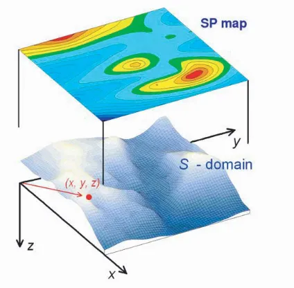
Let us consider a reference system with a horizontal (x, y)-plane placed at sea level and thez-axis positive downwards, and a 2D datum domain
S as in Figure 1. The S-domain is generally a non-flat ground survey area described by a topographic height function z(x, y). We indicate with ES(r) the SP electrical field vector at a set of datum points r≡[x, y, z(x, y)], with r∈S.
In areas with rough topography and inaccessible sites the current practice in collecting SP data consists of a continuous displacement of the measuring dipole along a generally irregular network of closed circuits and/or two-way interconnected branched lines. In order to provide a uniform and dense distribution of ES(r) data, a pre-processing is required according to the following three steps [2].
Figure 1. The datum domain (S-domain) generating the SP map on top. The (x, y)-plane is placed at sea level and thez-axis points into the earth.
by the spacings Δy and Δx, respectively. Along any ϕ-profile or ψ -profile, the sampling interval projection onto the (x, y)-plane, equal to Δx or Δy, respectively, is assumed constant and, for the sake of easier calculations, such that Δx = Δy = Δτ, where Δτ is taken from now on as the unique distance discretization element. Using a regular square grid on the (x, y)-plane, at each cross point of every pair of perpendicularx-line andy-line, a pair of values of the electrical field components, Eϕ(r) and Eψ(r), is assigned. These are estimated by interpolation from the SP map across dipoles of length Δϕ and Δψ, respectively and attributed to the midpoint of the projected dipoles, both of length Δτ. By indicating with ΔUϕ and ΔUψ the potential difference across Δϕand Δψ, respectively, we readily obtain the estimates of Eϕ(r) andEψ(r) as
Eϕ(r) =−
ΔUϕ(r) Δϕ =−
ΔUϕ(r)
Δτ
1 + (Δz/Δτ)2
1/2, (1a)
Eψ(r) =−
ΔUψ(r) Δψ =−
ΔUψ(r)
Δτ
1 + (Δz/Δτ)2
3. THE SP PROBABILITY TOMOGRAPHY THEORY
3.1. The SP Electric Field Vector Function and Its Power
We assume thatES(r) can be discretised as
ES(r) = M
m=1
(pm·Pm)s(r,rm) + N
n=1
(dun·Lun)s(r,rn)
+ G
g=1
quvg ·Suvg s(r,rg) + H
h=1
(ouvwh ·Cuvwh )s(r,rh), (2)
i.e., as a sum of effects due to:
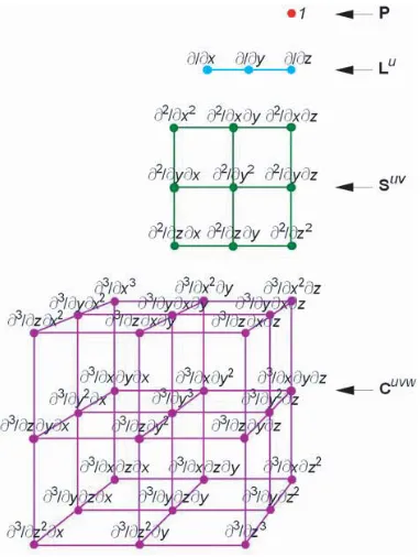
- a set of M poles, the mth element of which is located at rm ≡ (xm, ym, zm) and has strengthpm·Pm, wherepm andPm are the pole moment and a point operator 0th-order tensor, respectively; - a set ofN dipoles, whosenth element is located atrn≡(xn, yn, zn) with strength (dun·Lun) (u = x, y, z), where dun and Lun are the dipole moment and a line operator 1st-order tensor, respectively; - a set of G quadrupoles, whose gth element is located at rg ≡ (xg, yg, zg) with strength (quvg ·Suvg ) (u, v = x, y, z), where quvg and Suvg , respectively, are the quadrupole moment and a square operator 2nd-order tensor;
- a set of H octopoles, whose hth element is located at rh ≡ (xh, yh, zh) and has strength (ohuvw·Cuvwh ) (u, v, w=x, y, z), where ouvwh andCuvwh are the octopole moment and a cube operator 3rd-order tensor, respectively.
The dot in the definition of the source strength tensors indicates inner product. The operator tensorsP, Lu, Suv and Cuvw (u, v, w =
x, y, z) are made geometrically explicit in Figure 2.
The effect of the M, N, G and H source elements at a point r∈S is determined by the vector kernels(r,ri) (i=m, n, g, h), which represents the electrical field vector due to a point positive charge of unitary strength. The componentssϕ(r,ri) andsψ(r,ri) ofs(r,ri) over theS-domain are explicitly given as
sϕ(r,ri) =
(x−xi) + (z−zi)zx
(x−xi)2+ (y−yi)2+ (z−zi)2 3/2x
ϕ, (3a)
sψ(r,ri) =
(y−yi) + (z−zi)zy
(x−xi)2+ (y−yi)2+ (z−zi)2 3/2y
Figure 2. Explicit representation of the symbolic tensor operators appearing in the definition of the strengths of the pole, dipole, quadrupole and octopole source elements defined in Eq. (2).
where it iszx =∂z/∂x,zy =∂z/∂y, xϕ = dx/dϕ and yψ = dy/dψ. We define the information power Λ, associated with ES(r), over the surfaceS as
Λ =
S
ES(r)·ES(r)dS, (4a)
which, using Eq. (2), is expanded as
Λ= M
m=1 pm
S
ES(r)·s(r,rm)dS+ N
n=1
u=x, y, z
dun
S
ES(r)·
∂s(r,rn)
∂un
dS
+ G
g=1
u=x,y,z
v=x,y,z
quvg
S
ES(r)·
∂2s(r,rg)
∂ug∂vg
dS
+ H
h=1
u=x,y,z
v=x,y,z
w=x,y,z
ouvwh
S
ES(r)·
∂3s(r,rh)
∂uh∂vh∂wh
3.2. The SP Source Pole Occurrence Probability
We consider a generic mth integral of the first sum in Eq. (4b) and apply Schwarz inequality, thus obtaining
S
ES(r)·s(r,rm)dS 2
≤
S
ES2(r)dS
S
s2(r,rm)dS. (5)
Inequality (5) is used to define a source pole occurrence probability (SPOP) function as [2]
η(mp)=Cm(p)
S
ES(r)·s(r,rm)dS, (6a)
where
Cm(p)=
S
ES2(r)dS
S
s2(r,rm)dS −1/2
(6b)
ands(r,rm) has the role of source pole scanner. The explicit formulae of the components sϕ(r,rm) and sψ(r,rm) of s(r,rm) over the S -domain are those reported in Eq. (3a) and Eq. (3b), respectively, puttingi=m.
The 3D SPOP function, which satisfies the condition−1≤ηm(p) ≤ 1, is given as a measure of the probability of a source pole of strength
pm placed atrm, being responsible for the observed ES(r) field. Each
η(mp) indicates the occurrence probability of a positive, null or negative electrical charge in each location.
For computational purposes, we proceed as follows. We assume that the projection ofSonto the (x, y)-plane can be fitted to a rectangle
R of sides 2X and 2Y along thex-axis andy-axis, respectively. Using the topography surface regularization factor g(z) given by [2]
g(z) =
1 + (∂z/dx)2+ (∂z/dy)2 1/2
(7)
Eq. (6a) is definitely written as
ηm(p) =Cm(p) +X
−X
+Y
−Y
with
Cm(p)= +X
−X
+Y
−Y
ES2(r)g(z)dxdy· +X −X +Y −Y
s2(r,rm)g(z)dxdy −1/2
. (8b)
3.3. The SP Source Dipole Occurrence Probability
We take a genericnth integral of the second sum in Eq. (4b) and apply, as previously, Schwarz’s inequality to each u-component. We can thus define a source dipole occurrence probability (SDOP) function as [9]
ηn,u(d) =Cn,u(d) +X −X +Y −Y
ES(r)·
∂s(r,rn)
∂un
g(z)dxdy, (u=x, y, z) (9a)
with
Cn,u(d)= +X
−X
+Y
−Y
ES2(r)g(z)dxdy· +X −X +Y −Y
∂s(r∂u,rn) n
2g(z)dxdy
−1/2 . (9b)
Also η(n,ud) falls in the range [−1, 1]. Thus, at each rn,3 values of ηn,u(d) can be computed. They are interpreted as a measure of the probability of a single source dipole located atrn, being responsible of the whole ES(r) field. Each first derivative of s(r,rn) has the role of source dipole scanner. The first derivatives of the componentssϕ(r,rn) and sψ(r,rn) of s(r,rn) over the S-domain are derived, respectively, from Eq. (3a) and Eq. (3b) as
∂sϕ(r,rn)
∂xn
= 3(x−xn)A1,n(x, z)− |r−rn|
2 |r−rn|5
xϕ, (10a)
∂sϕ(r,rn)
∂yn
= 3(y−yn)A1,n(x, z)
|r−rn|5
xϕ, (10b)
∂sϕ(r,rn)
∂zn
= 3(z−zn)A1,n(x, z)− |r−rn|
2z
x
|r−rn|5
xϕ, (10c)
∂sψ(r,rn)
∂xn
= 3(x−xn)B1,n(y, z)
|r−rn|5
yψ, (10d)
∂sψ(r,rn)
∂yn
= 3(y−yn)B1,n(y, z)− |r−rn|
2 |r−rn|5
∂sψ(r,rn)
∂zn
= 3(z−zn)B1,n(y, z)− |r−rn|
2 zy |r−rn|5
yψ , (10f)
withA1,n(x, z) = (x−xn)+(z−zn)zx,B1,n(y, z) = (y−yn)+(z−zn)zy.
3.4. The SP Source Quadrupole Occurrence Probability
Accordingly, we consider now a genericgth integral of the third sum in Eq. (4b) and apply Schwarz’s inequality to each uv-element (u, v =
x, y, z), which allows a source quadrupole occurrence probability (SQOP) function to be defined as [10]
ηg,uv(q) =Cg,uv(q) +X −X +Y −Y
ES(r)·
∂2s(r,rg)
∂ug∂vg
g(z)dxdy, (11a)
with
Cg,uv(q) = +X
−X
+Y
−Y
ES2(r)g(z)dxdy· +X −X +Y −Y
∂2s(r,rg)
∂ug∂vg
2g(z)dxdy
−1/2
. (11b)
As before, the 3D SQOP function also falls in the range [−1, 1]. Thus, at each pointrg,9 values ofη(g,uvq) are taken as a measure of the probability for a quadrupole source located at rg, to be responsible of the ES(r) dataset. Since Suvg is a symmetric square tensor, it follows
thatη(g,uvq) =ηg,vu(q) . Therefore, at eachrg, the 3 diagonal plus the 3 right-up or left-down off-diagonal terms of ηg,uv(q) are sufficient. However, as we are interested in finding the position of the corners of a source body, we will finally consider only the 3 off-diagonal terms (u =v) [10].
Each second derivative ofs(r,rg) has the role of source quadrupole scanner. The useful second derivatives of the componentssϕ(r,rg) and
sψ(r,rg) of s(r,rg) over the S-domain are derived, respectively, from Eq. (3a) and Eq. (3b) as
∂2sϕ(r,rg)
∂xg∂yg =
3(y−yg)
5(x−xg)A1,g(x, z)− |r−rg|2
|r−rg|7
xϕ, (12a)
∂2sϕ(r,rg)
∂xg∂zg
=15(x−xg)(z−zg)A1,g(x, z)−3A2,g(x, z)|r−rg|
2 |r−rg|7
xϕ,(12b)
∂2sϕ(r,rg)
∂yg∂zg =
3(y−yg)
5(z−zg)A1,g(x, z)− |r−rg|2zx
|r−rg|7
∂2sψ(r,rg)
∂xg∂yg =
3(x−xg)
5(y−yg)B1,g(y, z)− |r−rg|2
|r−rg|7
yψ, (12d)
∂2sψ(r,rg)
∂xg∂zg =
3(x−xg)
5(z−zg)B1,g(y, z)− |r−rg|2zy
|r−rg|7
yψ , (12e)
∂2sψ(r,rg)
∂yg∂zg
=15(y−yg)(z−zg)B1,g(y, z)−3B2,g(y, z)|r−rg|
2 |r−rg|7
yψ (12f)
withA1,g(x, z) = (x−xg)+(z−zg)zx,A2,g(x, z) = (z−zg)+(x−xg)zx,
B1,g(x, z) = (y−yg) + (z−zg)zy andB2,g(x, z) = (z−zg) + (y−yg)zy. 3.5. The SP Source Octopole Occurrence Probability
Finally, we consider a generic hth integral of the fourth sum in Eq. (4b) and apply again Schwarz’s inequality to each uvw-term (u, v, w = x, y, z), allowing a source octopole occurrence probability (SOOP) function to be defined as
η(h, uvwo) =Ch, uvw(o) +X −X +Y −Y
ES(r)·
∂3s(r,rh)
∂uh∂vh∂wh
g(z)dxdy, (13a)
with
Ch,uvw(o) = +X
−X
+Y
−Y
ES2(r)g(z)dxdy· +X −X +Y −Y
∂u∂3s(r,rh) h∂vh∂wh
2g(z)dxdy
−1/2 . (13b)
As noted above, the 3D SOOP function falls in the range [−1, 1]. At each rh,27 values may now be calculated, each interpreted as a probability measure of a single octopole source located at rh, being responsible of the wholeES(r) dataset. However, as we are interested in finding only the position of the vertices of a source body, we will limit our analysis only to the SOOP function withu=v=w.
Each third derivative of s(r,rh) takes the role of source octopole scanner. The useful third derivatives of the componentssϕ(r,rh) and
sψ(r,rh) of s(r,rh) over theS-domain are derived, respectively, from Eq. (3a) and Eq. (3b) as
∂3s
ϕ(r,rh) ∂xh∂yh∂zh=
15(y−yh) 7(x−xh)(z−zh)A1,h(x, z)A2,h(x, z)|r−rh|2
|r−rh|9 xϕ, (14a) ∂3s
ψ(f ¯r,rh) ∂xh∂yh∂zh =
15(x−xh) 7(y−yh)(z−zh)B1,h(y, z)−B2,h(y, z)|r−rh|2
|r−rh|9 y
withA1,h(x, z) = (x−xh)+(z−zh)zx,A2,h(x, z) = (z−zh)+(x−xh)zx,
B1,h(x, z) = (y−yh) + (z−zh)zy andB2,h(x, z) = (z−zh) + (y−yh)zy. 4. SYNTHETIC EXAMPLES
We show some synthetic examples, in order to outline the main aspects of the multipole generalisation of the SP probability tomography.
4.1. The Coaxial Cube Model
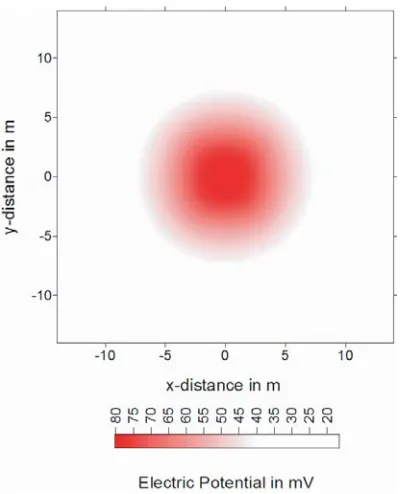
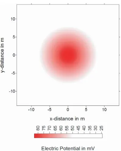
At first, we consider a coaxial cube model with sides 6 m long parallel to the coordinate axes and centre atx= 0,y= 0,z= 6 m. A positive charge of 0.5 C is assumed uniformly distributed on the surface of the cube with a charge surface density Δσ ∼= 2.315·10−3C/m2. The SP data have been computed at the nodes of a Cartesian grid where the elements are unit squares, using a 1 m step from −18 m to 18 m along both x-axis andy-axis. Figure 3 shows the synthetic SP map on the
Figure 3. The SP map for the cube model with a positive charge surface density Δσ ∼= 2.315·10−3C/m2, sides 6 m long and centre at
(a) (e)
(b) (f)
(c) (g)
(d) (h)
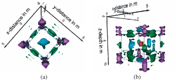
(a) (b)
Figure 5. A joint representation of the SPOP (red), SDOP (light blue), SQOP (green) and SOOP (purple) nuclei, viewed from top (a) and laterally (b), useful to retrieve the source body of the SP map in Figure 3.
(x, y)-plane.
Figure 4 shows the results from the application of the multipole probability tomography algorithm to the SP map in Figure 3. Since no topographic effects have been simulated, the scanner functions used to compute the η-functions have been obtained from the previous formulae putting zx = zy = 0, xϕ = yψ = 1 and g(z) = 1. For the sake of clarity, in all of the 3D probability tomography plots we will show sufficiently small SPOP, SDOP, SQOP and SOOP nuclei, each enclosing the maximum absolute value (MAV) of the corresponding
η-function.
The SPOP image shows a positive nucleus around the cube centre. The SDOP image shows, instead, three distinct doublets of nuclei with opposite signs very close to the centres of the corresponding opposite faces of the cube. Three distinct quadruplets appear around the centres of the cube sides in the SQOP tomographies of the off-diagonal terms, and an octoplet located at the vertices of the cube is the peculiar result from the SOOP image. The parameters of the nuclei in Figure 4 are listed in Table 1. A shift of 0.1 m alongz-axis is estimated for the cube centre from its true position. Furthermore, an average error of about 3% affects the estimate of the side length of the cube, from the distance between the MAV points of two opposite nuclei in each multiplet.
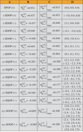
Table 1. Characterization of the SPOP, SDOP, SQOP and SOOP nuclei in Figure 4. A: nucleus type; B: selected bounding isosurface level; C: maximum absolute value (MAV); D: (x, y, z) of the MAV point.
A B C D
SPOP (+) m(p)=0.950
max ) (p
m =0.952 (0.0, 0.0, 5.9)
x-SDOP (+) n(d,x)=0.450
max ) ( , d x
n =0.491 ( 3.1, 0.1, 6.0)
x-SDOP ( ) n(d,x)= 0.440
max ) ( , d x
n =0.467 (3.1, 0.0, 6.0)
y-SDOP (+) n(d,y)=0.460
max ) ( , d y
n =0.494 ( 0.1, 3.0, 6.0)
y-SDOP ( ) n(d,y)= 0.440
max ) ( , d y
n =0.467 ( 0.1, 3.0, 6.0)
z-SDOP (+) n(,dz)=0.450
max ) ( , d z
n =0.481 (0.0, 0.1, 3.0)
z-SDOP ( ) n(d,z)= 0.450
max ) ( , d z
n =0.484 (0.0, 0.0, 9.0)
xy-SQOP (+) g(q,xy) =0.280
max ) ( , q xy
g =0.297 ( 3.0, 3.0, (3.0, 3.0, 5.9) 5.9)
xy-SQOP ( ) (gq,xy) = 0.280
max ) ( , q xy
g =0.297 (3.1, 3.0, ( 3.0, 3.0, 6.0) 6.0)
xz-SQOP (+) g(q,xz) =0.240
max ) ( , q xz
g =0.289 ( 3.3, 0.0, 3.1) (3.3, 0.0, 9.0)
xz-SQOP ( ) (gq,xz) = 0.240
max ) ( , q xz
g =0.284 ( 3.3, 0.0, 9.0) (3.3, 0.0, 3.1)
yz-SQOP (+) g(q,)yz=0.240
max ) ( , q yz
g =0.289 (0.0, 3.2, (0.0, 3.3, 9.0) 3.1)
yz-SQOP ( ) (gq,yz) = 0.240
max ) ( , q yz
g =0.284 (0.0, 3.2, (0.0, 3.2, 3.1) 9.0)
xyz-SOOP (+) h(o,xyz) =0.122
max ) ( , o xyz h =0.129
(3.1, 3.1, 3.0) ( 3.1, 3.1, 3.0)
(3.1, 3.1, 9.0) ( 3.1, 3.1, 9.0)
xyz-SOOP ( ) h(o,xyz) = 0.122
max ) ( , o xyz h =0.129
(3.1, 3.1, 3.1) ( 3.1, 3.1, 3.1) ( 3.1, 3.1, 9.1)
(3.1, 3.1, 9.0)
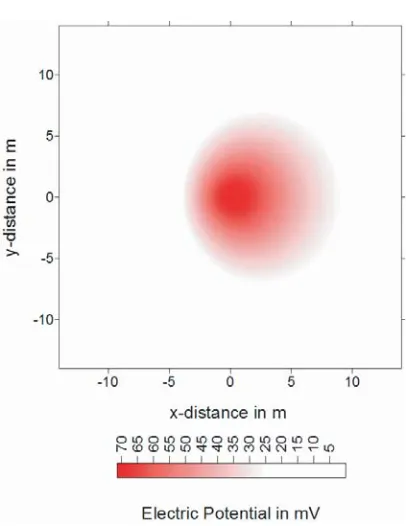
4.2. The Single Point Charge Model
The SP map in Figure 3 has a very close resemblance with the map due to a point charge. To this aim, we consider a point charge of 0.5 C placed at x = 0, y = 0, z = 6 m. The SP map has been computed at the nodes of a square grid with the same characteristics as in the previous case. Figure 6 depicts the SP map thus obtained.
Figure 7 shows the results from the application of the multipole tomography imaging. As in the coaxial cube case, the SPOP image gives a clear indication as to the correct position of the point charge. However, in spite of the fact that the source is a single pole, SDOP, SQOP and SOOP nuclei also appear so regularly located that, considered singularly, no difference can be detected with respect to the previous cube model. The situation changes considerably if we plot the SDOP, SQOP and SOOP nuclei altogether into a multipole image as in Figure 8. It is no longer possible, now, to combine a set of SDOP, SQOP and SOOP nuclei crossed by a single plane as in the previous case. In other words, a cube’s face can no longer be traced. The multipole analysis seems thus able to differentiate the response of a cube from that of a point source.
Figure 6. The SP map due to a point charge of 0.5 C placed atx= 0,
(a) (e)
(b) (f)
(c) (g)
(d) (h)
(a) (b)
Figure 8. A joint representation of the SPOP (red), SDOP (light blue), SQOP (green) and SOOP (purple) nuclei under two different angles of view, derived from the SP map in Figure 6.
The fact that SDOP, SQOP and SOOP nuclei are developed also for the single point charge model must be interpreted as the consequence of the probability meaning attributed to the η-functions. These functions allow the points where they obtain the maximum occurrence probability to be detected. An array of multipoles is thus highlighted, providing a SP response equivalent to that of a single point source. In other words, the multipole source geometry in Figure 8 is likely to represent the most probable polyhedral figure generating a SP response equivalent to that drawn in Figure 6. The parameters of the SPOP, SDOP, SQOP and SOOP nuclei are listed in Table 2.
4.3. The Rotated and Tilted Cube Model
We show now what happens when the sides of the cube are no longer parallel to the reference coordinate axes. A new model is thus analysed by rotating the cube previously dealt with by 45◦ around both the vertical z-axis and y-axis through the centre. Figure 9 shows the SP map of this new source body configuration.
Table 2. Characterization of the SPOP, SDOP, SQOP and SOOP nuclei in Figure 7. A: nucleus type; B: selected bounding isosurface level; C: maximum absolute value (MAV); D: (x, y, z) of the MAV point.
A B C D
SPOP (+) m(p)=0.931
max ) (p
m =0.933 (0.0, 0.0, 6.0)
x-SDOP (+) n(d,x)=0.437
max ) ( , d x
n =0.453 ( 3.0, 0.0, 6.0)
x-SDOP ( ) n(,dx)= 0.437
max ) ( , d x
n =0.448 (3.1, 0.0, 6.0)
y-SDOP (+) n(d,y)=0.440
max ) ( , d y
n =0.463 ( 0.1, 3.0, 6.0)
y-SDOP ( ) n(,dy)= 0.440
max ) ( , d y
n =0.448 (0.0, 3.0, 6.1)
z-SDOP (+) n(d,z)=0.445
max ) ( , d z
n =0.462 (0.1, 0.1, 3.1)
z-SDOP ( ) n(d,z)= 0.445
max ) ( , d z
n =0.464 (0.1, 0.1, 9.1)
xy-SQOP (+) (gq,xy) =0.283
max ) ( , q xy
g =0.300 ( 2.2, 2.3, (2.2, 2.2, 5.9) 5.9)
xy-SQOP ( ) (gq,xy) = 0.283
max ) ( , q xy
g =0.300 (2.2, 2.3, ( 2.2, 2.2, 5.9) 5.9)
xz-SQOP (+) (gq,xz) =0.150
max ) ( , q xz
g =0.177 ( 2.5, 0.2, (2.5, 0.1, 7.5) 4.5)
xz-SQOP ( ) (gq,xz) = 0.150
max ) ( , q xz
g =0.177 ( 2.5, 0.1, (2.5, 0.2, 4.5) 7.5)
yz-SQOP (+) (gq,yz) =0.160
max ) ( , q yz
g =0.177 ( 0.2, 2.5, ( 0.1, 2.5, 7.5) 4.6)
yz-SQOP ( ) (gq,yz) = 0.160
max ) ( , q yz
g =0.177 ( 0.1, 2.5, ( 0.2, 2.5, 4.5) 7.5)
xyz-SOOP (+) h(o,xyz) =0.085
max ) ( , o xyz h =0.100
(2.0, 2.1, 4.5) ( 2.0, 2.1, 4.4)
(1.9, 2.1, 7.6) ( 2.0, 2.1, 7.5)
xyz-SOOP ( ) h(o,xyz) = 0.085
max ) ( , o xyz h =0.100
(2.1, 2.0, 4.4) ( 2.0, 2.0, 4.4) ( 2.0, 2.0, 7.5)
(2.0, 2.0, 7.5)
Figure 9. The SP map for the tilted cube model with same parameters as in Figure 3, rotated by 45◦ around the vertical and horizontal axes through the centre.
homologous pairs. However, it must be stressed that this behaviour is not casual, since the procedure simply implies the search for the MAV points of the first, second and third order crossed derivatives of the kernel function with respect to the reference axes. When plotted altogether, the SDOP, SQOP and SOOP nuclei still make possible to delineate the cubic shape of the source body, as clearly visible in Figure 11.
4.4. The Coaxial Two-prism Model
(a) (e)
(b) (f)
(c) (g)
(h) (d)
(a) (b)
Figure 11. A joint representation of the SPOP (red), SDOP (light blue), SQOP (green) and SOOP (purple) nuclei, under two different angles of view, useful to retrieve the source body of the SP map in Figure 9.
square grid by a 1 m long step in the rectangle [−60,60]×[−30,30] m2. Figure 12 shows the SP maps for the three cases in order of decreasing distance between the centres from the top (a) to the bottom plot (b). It is quite evident that the decreasing distance is the cause of an increasing compression of the SP contour lines in the region of highest mutual interference.
Figure 13 displays the tomography results for the three cases, where, for brevity, only the combined multipole images are reported. In the top one, which refers to a distance between the centres greater than 3 times the average side length of the bodies, the interaction between the two prisms is rather negligible and their true shape can still be recognised. In the middle image, which refers to a distance between the centres of about 2.5 times the average side length, all of the facing SDOP, SQOP and SOOP nuclei depart from their initial places to converge to the centre of the two bodies’ system. Finally, in the bottom picture, which refers to a distance a little greater than 2 times the average side length, the detached facing nuclei of the same type are wholly melted midway between the prisms. The facing faces, corners and vertices of the two nearby bodies have therefore completely lacked resolution. This localised effect is not to be considered a weakness of the proposed multipole approach, but rather an intrinsic physical limitation due to the relatively small distance between the two bodies with respect to the depth of burial.
5. A FIELD CASE-HISTORY
Figure 12. The SP map for the two-prism model made of: (1) a cube with Δσ ∼= 5.787·10−4C/m2, sides parallel to the three coordinate axes and 12 m long each, and centre at x = 20 m (a), x = 14.5 m (b) and x = 11 m (c), y = 4 m, z = 15 m; (2) a parallelepiped with Δσ ∼= −4.822·10−4C/m2, x- and z-oriented sides 13 m long and y
(b)
(a)
(c)
Figure 13. A joint representation of the SPOP (red), SDOP (light blue), SQOP (green) and SOOP (purple) nuclei for the two-prism model with decreasing distance between the centres of the two prisms. The sequence of the images is the same as that of the SP maps in Figure 12.
volcanic areas, SP positive anomalies correspond to upward migrating fluids, while negative ones to a downward fluid movement [9, 14].
We illustrate now the application of the SP 3D multipole probability tomography to an SP survey carried in the volcanic area of Mt. Somma-Vesuvius (Naples, Italy), which aimed to configure the main plumbing system of the volcanic complex. Mt. Somma-Vesuvius is a polygenic strato-volcano, whose most recent period of history (1631–1944) was characterized by a semipersistent, relatively mild activity (lava fountains, gases and vapour emission from the crater), frequently interrupted by short quiet periods that never exceeded seven years. From 1944 to the present time, Mt. Somma-Vesuvius has remained quiet.
Figure 14. The Mt. Somma-Vesuvius survey area.
sketched in Figure 14. Figure 15 shows the behaviour of the SP field in mV, resulting from the processing of 1250 measurements [15, 16]. As the area is characterized by a strongly uneven topography, the 3D multipole tomography algorithm with topographic effects has been used. A similar SP map realised in 1995 was elaborated by the probability tomography method, limitedly, however, only to the source pole and dipole analysis [9, 15, 16].
The SPOP image in Figure 16 displays a pair of nuclei of opposite sign containing two poles with the highest occurrence probability. They are interpreted as the centres of the polarised bodies responsible of the SP biggest anomalies of opposite sign drawn in Figure 15. The negative and positive poles appear located, respectively, beneath the Somma caldera northern rim and the Vesuvius cone. Combining in pairs and altogether the SPOP, SDOP, SQOP and SOOP nuclei into single plots, the images in Figure 17 are obtained.
Table 3. Coordinates in km of the points with relative maximum absolute values for the SPOP, SDOP, SQOP and SOOP nuclei in Figure 17.
Anomaly SPOP (+) SPOP ( )
SPOP (5.4, 6.3, 1.5) (6.5, 9.9, 0.9) x-SDOP (+) (4.3, 6.2, 1.6) (7.3, 10.0,1.0) x-SDOP ( ) (6.9, 6.2, 1.6) (5.4, 9.8, 1.0) y-SDOP (+) (5.3, 5.4, 1.8) (6.3, 11.6, 1.0) y-SDOP ( ) (5.3, 7.0, 1.7) (6.4, 9.0, 0.9) z-SDOP (+) (5.5, 6.3, 0.9) (6.4, 9.9, 1.9) z-SDOP ( ) (5.5, 6.3, 2.7) (6.5, 9.9, 0.4)
xy-SQOP (+) (4.6, 5.5, 1.8) (6.5, 6.9, 1.8)
(5.5, 9.0, 1.2) (7.1, 11.5, 1.3)
xy-SQOP ( ) (4.6, 6.9, 1.8) (6.6, 5.5, 1.8)
(5.5, 11.3, 1.2) (7.1, 9.0, 1.3)
xz-SQOP (+) (4.5, 6.0, 0.9) (6.5, 6.1, 2.7)
(5.4, 9.7, 0.2) (7.4, 10.2, 2.1)
xz-SQOP ( ) (6.5, 6.0, 0.8) (4.6, 6.1, 2.7)
(7.2, 9.9, 0.2) (5.2, 10.2, 2.2)
yz-SQOP (+) (5.4, 5.2, 0.7) (5.4, 7.2, 2.6)
(6.3, 9.0, 0.3) (6.2, 11.6, 2.1)
yz-SQOP ( ) (5.2, 7.1, 0.7) (5.4, 5.2, 2.6)
(6.3, 11.3, 0.2) (6.3, 9.1, 2.1)
xyz-SQOP (+)
(4.5, 6.8, 0.7) (6.3, 5.3, 0.7) (4.7, 5.6, 2.7) (6.4, 7.0, 2.7)
(5.4, 8.8, 0.3) (6.9, 11.0, 0.2) (5.5, 11.2, 1.9) (7.0, 9.3, 2.0)
xyz-SQOP ( )
(4.6, 5.3, 0.7) (6.3, 5.6, 0.7) (4.7, 7.1, 2.7) (6.4, 6.8, 2.7)
(5.4, 10.8, 0.1) (6.9, 8.8, 0.3) (5.5, 9.3, 2.0) (7.0, 11.5, 2.3) _ − − − − − − − −
the SPOP, SDOP, SQOP and SOOP nuclei in Figure 17 are listed in Table 3, from which the source bodies are estimated to be confined within the first 3 km of depth b.s.l.
meteoric water, percolate, should reasonably correspond with the negatively charged block beneath the Somma caldera northern rim. The ascending branch, where the fluids heated from below rise up, should instead correspond with the positively charged block beneath the Vesuvius cone, and likely form the reservoir feeding the active fumaroles located in the top central crater.
Figure 15. The Mt. Somma-Vesuvius SP map.
(d) (a) (b)
(c)
Figure 17. A joint representation of the SPOP and SDOP (a), SPOP and SQOP (b), SPOP and SOOP (c), SPOP, SDOP, SQOP and SOOP (d) nuclei, resulting from the application of the 3D multipole tomography method to the Mt. Somma-Vesuvius SP map in Figure 17.
6. CONCLUSION
We have exposed the theory of the 3D multipole probability tomography for the SP method by a generalised approach including a combination of poles, dipoles, quadrupoles and octopoles as elementary point sources of the SP anomalies. These physical sources have been used to detect the position of the centres of the true sources and to highlight the features of their boundaries. Improving the geometrical definition of the sources of the SP anomalies has thus been the main purpose of the new approach.
volcanology, as in this study, seismology [17] and archaeology [10, 11]. We also stress the importance that the probability tomography can have in the study of the time evolution of the SP signals in high-risk volcanic areas, where the electrokinetic source field may undergo a rapid increase of intensity in conjunction with an increase of the volcanic emission activity. The 4D tomography is in fact becoming a very promising monitoring technique especially in fast flow visualization [18].
REFERENCES
1. Patella, D., “Introduction to ground surface self-potential tomography,”Geophys. Prosp., Vol. 45, 653–681, 1997.
2. Patella, D., “Self-potential global tomography including topo-graphic effects,”Geophys. Prosp., Vol. 45, 843–863, 1997.
3. Mauriello, P. and D. Patella, “Resistivity anomaly imaging by probability tomography,”Geophys. Prosp., Vol. 47, 411–429, 1999. 4. Mauriello, P. and D. Patella, “Principles of probability tomography for natural-source electromagnetic induction fields,”
Geophysics, Vol. 64, 1403–1417, 1999.
5. Mauriello, P. and D. Patella, “Gravity probability tomography: A new tool for buried mass distribution imaging,”Geophys. Prosp., Vol. 49, 1–12, 2001.
6. Mauriello, P. and D. Patella, “Localization of maximum-depth gravity anomaly sources by a distribution of equivalent point masses,”Geophysics, Vol. 66, 1431–1437, 2001.
7. Mauriello, P. and D. Patella, “Localization of magnetic sources underground by a probability tomography approach,”Progress In Electromagtics Research M, Vol. 3, 27–56, 2008.
8. Mauriello, P. and D. Patella, “Resistivity tensor probability tomography,”Progress In Electromagtics Research B, Vol. 8, 129– 146, 2008.
9. Mauriello, P. and D. Patella, “Geoelectrical anomalies imaged by polar and dipolar probability tomography,” Progress In Electromagtics Research, PIER 87, 63–88, 2008.
10. Alaia, R., D. Patella, and P. Mauriello, “Application of the geoelectrical 3D probability tomography in a test-site of the archaeological park of Pompei (Naples, Italy),”J. Geophys. Eng., Vol. 5, 67–76, 2008.
Ap-plication to near surface geoelectrical surveys,”J. Geophys. Eng., Vol. 5, 359–370, 2008.
12. Landau, L. D. and E. M. Lifˇsits,Elektrodinamika Sploˇsnych Sred, Nauka, Moscow, 1982.
13. Corwin, R. F., “The self-potential method for environmental and engineering applications,” Geotechnical and Environmental Geophysics, S. H. Ward (ed.), Chap. 1: Review and Tutorial, SEG, 127–146, Tulsa, 1990.
14. Saracco, G., P. Labazuy, and F. Moreau, “Localization of selfpotential sources in volcano-electric effect with complex continuous wavelet transform and electrical tomography methods for an active volcano,” Geophys. Res. Lett., Vol. 31, 1–5, 2004. 15. Di Maio, R., P. Mauriello, D. Patella, Z. Petrillo, S. Piscitelli, and
A. Siniscalchi, “Electric and electromagnetic outline of the Mount Somma-Vesuvius structural setting,” J. Volcanol. Geoth. Res., Vol. 82, 219–238, 1998.
16. Iuliano, T., P. Mauriello, and D. Patella, “Looking inside Mount Vesuvius by potential fields integrated geophysical tomographies,”
J. Volcanol. Geoth. Res., Vol. 113, 363–378, 2002.
17. Lapenna, V., D. Patella, and S. Piscitelli, “Tomographic analysis of self-potential data in a seismic area of southern Italy,”
Ann. Geofis., Vol. 43, 361–374, 2000.