Cryptanalysis of HFE, Multi-HFE and Variants for Odd and Even Characteristic

(1)

Cryptanalysis of HFE, Multi-HFE and Variants for Odd and

Even Characteristic

Luk Bettale?, Jean-Charles Faug`ere, and Ludovic Perret

INRIA, Paris-Rocquencourt Center, SALSA Project UPMC Univ Paris 06, UMR 7606, LIP6, F-75005, Paris, France

CNRS, UMR 7606, LIP6, F-75005, Paris, France

[email protected], [email protected], [email protected]

Abstract. We investigate in this paper the security of HFE and Multi-HFE schemes as well as their minus and embedding variants. Multi-HFE is a generalization of the well-known HFE schemes. The idea is to use a multivariate quadratic system – instead of a univariate polynomial in HFE – over an extension field as a private key. According to the authors, this should make the classical direct algebraic (message-recovery) attack proposed by Faug`ere and Joux on HFE no longer efficient against HFE. We consider here the hardness of the key-recovery in Multi-HFE and its variants, but also in Multi-HFE (both for odd and even characteristic). We first improve and generalize the basic key recovery proposed by Kipnis and Shamir on HFE. To do so, we express this attack as matrix/vector operations. In one hand, this permits to improve the basic Kipnis-Shamir (KS) attack on HFE. On the other hand, this allows to generalize the attack on Multi-HFE. Due to its structure, we prove that a Multi-HFE scheme has much more equivalent keys than a basic HFE. This induces a structural weakness which can be exploited to adapt the KS attack against classical modifiers of multivariate schemes such as minus and embedding. Along the way, we discovered that the KS attack as initially described cannot be applied against HFE in characteristic 2. We have then strongly revised KS in characteristic 2 to make it work. In all cases, the cost of our attacks is related to the complexity of solving MinRank. Thanks to recent complexity results on this problem, we prove that our attack is polynomial in the degree of the extension field for all possible practical settings used in HFE and Multi-HFE. This makes then Multi-HFE less secure than basic HFE for equally-sized keys. As a proof of concept, we have been able to practically break the most conservative proposed parameters of multi-HFE in few days (256 bits security broken in 9 days).

Keywords: Hidden Field Equations, MinRank, Gr¨obner bases

1 Introduction

The problem of finding a low rank linear combination of matrices is a basic linear algebra problem [12] known as MinRank in cryptography [16]. This problem is NP-hard [12] and has been used to design a zero-knowledge authentication scheme [16]. More generally, it appears that MinRank is underlying the security of several cryptographic schemes [32, 15]. A well known example is the key recovery attack of the multivariate scheme HFE [38] (Hidden Field Equations) proposed by Kipnis and Shamir [32] who showed that the security of HFE can be reduced to the difficulty of MinRank. Their technique is usually called Kipnis-Shamir’s attack, or KS attack. They also proposed a general algorithm to solve MinRank. The idea is to map an instance of MinRank to an algebraic system. They then proposed an “ad-hoc” technique to solve such polynomial systems.

Later, Faugère, Levy-dit-Vehel and Perret [26] improve Kipnis-Shamir’s attack by using Gröbner bases [9, 10, 11] techniques. In particular, they noticed that the system arising in Kipnis-Shamir’s attack has a very specific structure: it is “bilinear”. This means that each equation of the system is the product of linear forms with distinct variables. Soon after, Faugère, Safey El Din and Spaenlehauer [28] presented a detailed study of the complexity of solving bilinear

?

(2)

systems with Gr¨obner bases. In particular, [28] proved that (generic or random) bilinear systems are much easier to solve than (generic) algebraic systems of the same size.

However, it seems reasonable to believe that polynomial systems occurring in cryptographic applications (such as in MinRank) are likely not generic; motivating then a dedicated analysis for important cases. In [27], MinRank instances occurring in authentication schemes have been further studied. In this paper, we consider instances of MinRank occurring in the cryptanalysis of multivariate public-key schemes.

Multivariate Public-Key Cryptography (MPKC) is the set of asymmetric schemes using the NP-hardness of solving a quadratic system of multivariate algebraic equations [29]. Mul-tivariate schemes are often considered as possible “low-cost” alternatives [36] to number the-ory based public key schemes. Their encryption/decryption procedures are very efficient and can be done in constrained environments [7, 13]. The main drawback is that the public key is rather large. Indeed, the one-way function is defined by a set of m quadratic polynomials (g1(x1, . . . , xn), . . . , gm(x1, . . . , xn)) ∈ K[x1, . . . , xn]m. Namely, the public operation is the

ap-plication

G: (v1, . . . , vn)∈Kn7→(g1(v1, . . . , vn), . . . , gm(v1, . . . , vn))∈Km.

To introduce a trapdoor, we choose a transformationF given by a system of algebraic equations (f1, . . . , fm)∈K[x1, . . . , xn]m. Thanks to a well chosen structure, the system is easy to solve. Let

GLn(K) be the group of invertible linear transformations and let Affn(K)'GLn(K)×Knbe the

space of invertible affine transformations. This structure is hidden by two affine transformations

S ∈Affn(K) andT ∈Affm(K) represented by matricesS and T. The public key is then:

G=T ◦ F ◦ S

(g1, . . . , gm) = (f1((x1, . . . , xn) S), . . . , fm((x1, . . . , xn) S))T.

In such schemes, the transformationsS,T and (usually)Fare kept secret andGis made public. To encrypt a message m= (m1, . . . , mn)∈Kn, we compute:

c= (c1, . . . , cm) = (g1(m1, . . . , mn), . . . , gm(m1, . . . , mn))∈Km.

To decrypt, the owner of the secret key inverts separately each component. AsS,T andF are easy to invert, this is done efficiently. The first multivariate scheme C* has been introduced by Matsumoto and Imai [34] and broken by Patarin [37]. After that, several trapdoor functions have been proposed in this framework [38, 33, 35, 40]. HFE probably remains the most famous one. In this paper we focus on the HFE and Multi-HFE structure introduced in [38, 6, 14].

In the original HFE [38], the secret inner system is the representation of a univariate poly-nomial over some extension of degree n ∈_N of a finite field Fq. This polynomial is chosen to

be easy to solve (low degree) and has a special structure that allows to have only quadratic polynomials in its (multivariate) small field representation. A practical message recovery at-tack [23, 25] and a theoretical key recovery [32] undermined the security of this scheme. To tackle these attacks, a generalization of HFE that uses a system ofN equations inN variables (instead of one univariate polynomial) in an extension field of degreedhas been proposed in [6] and in [13]. In this paper, we call this construction Multi-HFE. The basic HFE scheme is then an instantiation of Multi-HFE withN = 1, d=n.

1.1 Main results

(3)

that the MinRank can be expressed in the small field and directly on the quadratic forms of the public key (g1, . . . , gn) ∈ Fq[x1, . . . , xn]n. This allows to considerably speed up the solving

step (for instance we have a speedup factor of 424 for q = 31 and n= 19) and also simplifies the KS attack. Due to its simpler description, we are able to generalize our attack to Multi-HFE (N >1) in odd-characteristic. These results were first published in [5] and concerns only odd-characteristic fields. In characteristic 2, there is no symmetric quadratic form representing a quadratic polynomial, and contrarily to what was stated in [32], KS attack does not work as initially described. Using the specificity of the problem in characteristic 2 and the possibility to add the field equations, we give two methods for adapting our attack in characteristic 2 depending on the parity of the target rank of the MinRank. Note that our adaptation applies both for HFE and Multi-HFE.

The MinRank problems occurring are very specific. First, a certain degree of freedom is left for its solving. This is related to a large amount of equivalent keys in HFE/Multi-HFE. We isolated two kind of transformations allowing to build equivalent keys. These transformations generalizes those given in [42, 43] for HFE. We show that an equivalent key has a canonical rep-resentation in terms of these transformations. As a direct consequence, we give a lower bound on the number of equivalent key for Multi-HFE, more precise than the one given in [5]. Second, the MinRank considered are greatly over-determined. Thanks to recent results on MinRank [26, 27], bilinear systems [28] and a new expression of the Hilbert function using orthogonal polynomials, we provide a precise complexity analysis of our attack. For all proposed practical parameters, we prove that the attack is polynomial in d, the degree of the extension and linear in log(q), just as we conjectured in [5].

Another consequence of equivalent keys is the possibility to attack two variants of Multi-HFE, namely Multi-HFE- and Multi-HFE with embedding. In Multi-HFE-, several polynomials are removed from the public keys. We show that only (n−N) matrices are needed to solve the MinRank problem instead ofn. These N degrees of freedom in the MinRank problem allow to perform our key recovery with no additional cost as the rank property still holds as long as the number of removed equations does not exceed N. For the embedding variant, the public polynomials have less variables leading to matrices with fewer rows and columns. However, a low rank linear combination of the quadratic forms can still be found. In this case, the matrixS

(corresponding to the change of variable) recovered is rectangular. In order to make it invertible, we need to extend this matrix in a special way to keep the shape of F unchanged.

All in all, for the same size of keys, the Multi-HFE family seems to be less secure than the original HFE (N = 1). As a proof of concept, we provide a practical key recovery on the most conservative parameters (256-bit security) proposed in [14] in less than 10 days.

1.2 Organization of the Paper

(4)

2 Preliminaries

LetKbe a field. Throughout this paper, we use the following conventions: an underlined letter

denotes a vector, e.g. v = (v1, . . . , vn) ∈ Kn. A capital bold font letter denotes a matrix, e.g.

M∈ M_n×n(K) where Mn×n(K) denotes the set ofn×nmatrices whose entries lie inK. We

also write M = [mi,j] to denote that the (i, j)-th coefficient of the matrix M is mi,j ∈ K for

0 6 i, j < n. We will also indifferently use ker (M) to denote the left kernel of M or (more often) a matrix whose rows form a basis of its left kernel. A calligraphic capital letter denotes a general mapping, e.g.F. The set of invertible matrices of Mn×n(K) is denoted by GLn(K).

The space of affine invertible transformations is denoted by Affn(K)'GLn(K)×Kn.

2.1 Multi-HFE

The parameters considered are (q, N, d, D) ∈ _N4_{. Here,} _q _{denotes the size of the ground field}

Fq,dis the degree of the extension field Fqd,N is the number of variables and equations of the

secret polynomials in the ringFqd[X₁, . . . , X_N], andDtheir degree. In the rest of the paper, we

use capital letters for elements relative to the extension Fqd (a.k.a. “big field” in this paper),

e.g.Vi ∈Fqd,F_i ∈_F_qd[X₁, . . . , X_N], and small letters for elements relative to _F_q (a.k.a. “small

field”), e.g.vi ∈Fq,fi ∈Fq[x1, . . . , xn]. To build the trapdoor function F, we use the following

transformation over the big field

F∗ : (V1, . . . , VN)∈(Fqd)N 7→(F₁(V₁, . . . , V_N), . . . , F_N(V₁, . . . , V_N))∈(_F_qd)N

with Fk ∈ Fqd[X₁, . . . , X_N],∀k,1 6 k 6 N, and deg (F_i) 6 D. In addition, the polynomials

F1, . . . , FN are constructed in a specific way. For all k,16k6N:

Fk= X

16i6j6N X

06u,v<d qu_+qv₆_D

Ak,i,u, j,v

X_iquX_jqv+ X

16i6N X

06u<d qu₆_D

Bk,i,uXq u

i +Ck,

where Ak,i,u, j,v

, Bk,i,u, Ck ∈ Fqd,∀i, j,1 6 i, j 6 N,∀u, v,0 6 u, v < d. From now on, we say

that such systems have (multi-)HFE-shape. For convenience, we denoten=N d. Let ϕN be a

morphism from (Fqd)N to_Fn_q. The transformation F use the small field representation of the

secret polynomials,F =ϕN ◦ F∗◦ϕ−_N1 with

F : (v1, . . . , vn)∈Fnq 7→(h1(v1, . . . , vn), . . . , hn(v1, . . . , vn))∈Fnq.

Due to the HFE-shape, each polynomial hi, for i,16i6nhas total degree 2.

The original HFE scheme [38] is mostly used over F2 and always with a single univariate

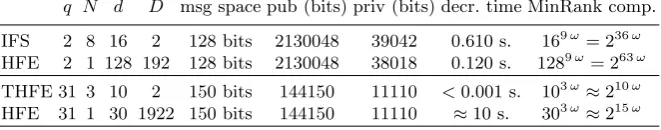
polynomial as a secret map. It is then an instantiation of multi-HFE withq= 2 andN = 1. The construction PHFE [19] (for projected HFE) is an odd characteristic univariate HFE that uses the embedding modifier (see Sect. 8.2). The scheme IFS [6] (for Intermediate Field System) is a multi-HFE in characteristic 2 and THFE [14] is a multi-HFE in odd characteristic (possibly with embedding modifier). To make the decryption efficient, all instances of multi-HFE with N > 1 use quadratic polynomials as internal secret transformations. In Table 1, we provide sample of parameters from the literature.

We briefly review known attacks against HFE/multi-HFE.

2.2 Direct Algebraic Attack

Let (c1, . . . , cn) ∈ Fnq be a ciphertext. A message-recovery attack in a multivariate scheme

(5)

Table 1.Parameters of various Multi-HFE instances found in several papers.

q N d D security HFE [38] 2 1 128 513 128 PHFE [19] 7 1 67 56 201 IFS [6] 2 8 16 2 128 THFE [14] 31 3 10 2 150

the gi’s are the public polynomials. A classical way to solve algebraic systems is to compute

a Gr¨obner basis [9, 10, 11, 1, 17]. The historical method for computing such bases has been proposed by Buchberger in his PhD thesis [9]. The algorithms F4 [21] and F5 [22] by Faug`ere

permit to improve the basic Buchberger’s algorithm. A good measure of the complexity for Gr¨obner bases is the so-called “degree of regularity” of a system. This can be viewed as the maximum degree of the polynomials appearing during the computation (see [2, 3]).

It appeared [23, 25] that inverting the public key of the original HFE is much easier than expected (i.e. in comparison to a random system of the same size). For original HFE, the degree of regularity has been experimentally shown to be roughly log_q(D) (see [25]). This makes the attack sub-exponential in the number of variables. Further analysis [30] confirmed this result. Note that the field equations (i.e. xq₁ −x1 = . . . = xqn−xn = 0) are mandatory to achieve

this complexity. Their role is to force the solutions to be only in the base field Fq. To prevent

a direct algebraic attack, it has been proposed [19] to use a field with a bigger characteristic. During the Gr¨obner basis computation, field equations only intervene in degree at leastq. Note that the hybrid approach described in [4] has been especially designed to solve such systems (for “intermediate” fields). As an example, for n= 28 and q= 31 the complexity of the hybrid approach is 282. It is better than a direct solving (2115) but the attack remains impractical.

More specifically, a HFE system with q > n is very hard to solve with a direct approach such as in [25] (for nsufficiently big). This intuition has been recently confirmed in [20] where the authors extend the analysis of [30] for all fields. After this, [18] produces an explicit bound on the degree of regularity which is

(q−1)dlog (D)e

2 + 2.

We remark that this bound is linear inq. This makes the cost of a direct Gr¨obner basis computa-tion exponential inqand then useless for a big enough field. For example, HFE with parameters q= 23, D= 1058 andn= 120, the (upper) bound on the degree of regularity according to [18] is 35. The corresponding cost for mounting a direct message-recovery attack is then 2242 opera-tions. For a comparison, the key-recovery attack presented in this paper will need 228operations for the same parameters.

For multi-HFE, there are less results. In characteristic 2, multi-HFE can still be attacked similarly to HFE as pointed in [6]. This confirms that the algebraic attack is somehow “optimal” overF2. However, as for basic HFE, the direct algebraic attack does not affect instantiations of

multi-HFE with bigger odd characteristic.

2.3 Original Kipnis-Shamir Attack

We now describe the key recovery attack proposed in [32] against the original HFE scheme (N = 1, n = d). The starting idea is to remark that the polynomials of the public key – as well as the transformations S,T – can be viewed as mappings G∗_,_S∗_,_T∗ _:

Fqn 7→ _F_qn and

(6)

then becomes

G=G∗(X) =T∗(F∗(S∗(X))).

Kipnis and Shamir [32] proposed interpolation to recover a univariate representation of the public key. We present a more efficient and simpler way in Sect. 3 to perform this step.

Kipnis and Shamir [32] also showed that the univariate polynomials can be written as a “non-standard quadratic form”. For instance, we have:

G=

n−1 X

i=0 n−1 X

j=0

gi,jXq i_+qj

=XGXt, whereX = (X, Xq, . . . , Xqn−1)

and G = [gi,j] ∈ Mn×n(Fqn). Note that this representation does not work in characteristic

2. In this section and in Sect. 3, we assume then that q is odd. The characteristic 2 case is addressed in Sect. 6.3. Similarly, we define F = [fi,j] ∈ Mn×n(Fqn) as the symmetric matrix

representation of the secret univariate polynomial.

The Kipnis-Shamir attack is based on the remark that the rank of F is bounded, namely Rank F 6 log_q(D). Indeed, the degree of the secret polynomial is smaller than D and the entriesfi,jinFare non-zero only ifi, j6logq(D). In addition, we writeT∗−1(X) =Pn

−1 k=0tkXq

k

and S∗_{(X) =}Pn−1 k=0skXq

k

.

The equationG∗(X) =T∗(F∗(S∗(X))) implies the so-called “Fundamental Equation” (see [32] for the proof):

n−1 X

k=0

tkG∗k =G0=WFf Wft, (1)

where Wf = [w_e_i,j]∈ M_n×n(Fqn) is a specified invertible matrix such that e

wi,j = sq i

(j−i) modn,

for alli, j,06i, j < n. Finally, for a given k,06k < n,G∗kis the matrix whose (i, j)-th entry isg_(iqk₋_{k) mod}_n,(j₋_{k) mod}_n, for all i, j,06i, j < n. As the rank of Fis bounded, so is the rank of

G0. Recovering the tk’s reduces to solve a MinRank problem.

Once the tk’s of (1) are known, thesk’s are recovered by solving a linear system. From (1),

we see that ker(G0) = ker(WFf ) and thus ker(G0)Wf = ker(F). Let ` = dlog_q(D)e, we recall

that only the upper left `×` submatrix of F has non-zero coefficients. Thus, any (n−`)×n matrix K whose first ` columns are 0 ensures KF=0. Furthermore, if Rank(F) = ` and the rows of Kare chosen linearly independent, then their rows form a basis of ker(F).

In any case, this is enough to ensure that the ` first columns of ker(G0)Wf are zero. This

gives rise to a linear system of equations overFqn of`(n−`) equations in then2 coefficients of f

W. In addition,Wf has the following shape:

f

W=



         

e

w0,0 we0,1 . . . we0,n−2we0,n−1

e

wq_0,n₋₁ we q 0,0 we

q

0,1 . . . we q 0,n−2

. .. . .. . ..

. . . w_e_0,nqn−₋2₂w_e_0,nqn−₋2₁ w_e_0,0qn−2 w_e_0,1qn−2

e

wq_0,1n−1 . . . w_eq_0,nn−₋1₂w_e_0,nqn−₋1₁ w_e_0,0qn−1



         

.

This is due to the fact thatw_ei+1,j+1=sq i+1

(j+1)−(i+1) =

sq_(ji₋_i)q=w_e_i,jq . Thus, Kipnis and Shamir proposed to reinterpret the equations overFq. This givesn `(n−`) equations in onlyn2 variables

over Fq. Solving this overdetermined system completes the key recovery. The main (and more

(7)

2.4 The MinRank Problem

The (square) MinRank problem over a finite field Kis defined as follows:

MinRank (MR)

Input:n, r, k∈Nand M0,M1, . . . ,Mk∈ Mn×n(K).

Question: Find – if any – a k-tuple (λ1, . . . , λk)∈Kk such that:

Rank

k X

i=1

λiMi−M0

!

6r.

We review below known algebraic techniques to solve this problem.

Kipnis-Shamir Modeling Kipnis and Shamir [32] proposed to formulate MinRank as a mul-tivariate polynomial system of equations. With the previous notations, solving MinRank over a finite field Kis equivalent to solving the algebraic system ofn(n−r) equations in r(n−r) +k

variables given by the entries of the matrix



 

1 x1,1 . . . x1,r

. .. .._. .._. 1xn−r,1. . . xn−r,r



 ·

k X

i=1

λiMi−M0

!

.

Solving this system is equivalent to find a left kernel (in echelon form) of

Pk

i=1λiMi−M0

.

This left kernel can be written in such a systematic form with high probability over a finite field. Initially, relinearization [32] has been used to solve this algebraic system. The authors of [26] proposed instead to use Gr¨obner bases tools to solve this system. In addition, [26] noticed that the system has a specific structure: it is formed by bilinear equations [28].

Minors Modeling Alternatively, MinRank is equivalent to finding a vector (λ1, . . . , λk)∈Kk

vanishing all the minors of size r + 1 of the matrix

Pk

i=1λiMi−M0

are zero. We have

then to solve a multivariate polynomial system of _r+1n 2 equations in k variables as pointed in [26, 27]. The system has more equations and less variables than the Kipnis-Shamir modeling but the degree of the equations isr. However, it seems that this approach is more efficient [27] (at least for MinRank instances used in the authentication scheme [16]). In addition, precise complexity bounds can be derived for this modeling [27].

Complexity. We recall the complexity of the F5 algorithm as given in [2, 3].

Theorem 1. The complexity of computing a Gr¨obner basis of a zero-dimensional (i.e. with a finite number of solutions in the algebraic closure of the coefficient field) polynomial system of m equations in n variables with F5 is

O

n+dreg

dreg ω

,

where dreg is the degree of regularity of the ideal and 26ω63 the linear algebra constant.

Informally,dregis the maximum degree reached during a Gr¨obner basis computation. For random

instances of square (m = n) quadratic systems, it holds that dreg = n+ 1 (see [2]). It has to

(8)

We consider now MinRank systems obtained by the minors modeling, Corollary 3 of [27] gives a bound on the degree of regularity of these particular systems. Note that this bound is also an upper bound for the degree of regularity of the Kipnis-Shamir modeling [27].

Proposition 1 (Faug`ere, Safey El Din, Spaenlehauer [27]). Let (n, r, k) be the param-eters of a MinRank instance. Let A(t) = [ai,j(t)] be the (r×r)-matrix defined by ai,j(t) = Pn−max(i,j)

`=0

n−i `

n−j `

t`. The degree of regularity of MinRank polynomial systems is bounded from above by 1 + deg (HS(t)) where HS(t) is the polynomial obtained from the first positive terms of the series

(1−t)(n−r)2−k detA(t) t(r2)

.

In Sect. 7, we will see that Proposition 1 is useful to bound the complexity of MinRank problems coming from HFE/multi-HFE.

3 Improvement and Generalization of the MinRank Attack

To generalize the MinRank attack proposed by Kipnis and Shamir [32], it is convenient to interpret it as matrix/vector operations. In what follows, we denote by Frobkthe function raising

all the components of a vector (or a matrix) to the power qk in any field Kof characteristicq.

For example, for a vector v= (v1, . . . , vm)∈Km, we have Frobk(v) = (vq k

1 , . . . , v qk

m)∈Km. For

a matrix A = [ai,j] ∈ Mn×n(K), we have Frobk(A) = [aq k

i,j]∈ Mn×n(K). In this section, we

will suppose that the characteristic of the fieldFq is different than two. This particular case is

addressed in Sect. 6.3.

3.1 Improving the Univariate Case

To express the KS attack as matrix/vector operation, we introduce the following change basis matrix.

Proposition 2. Let(θ1, . . . , θn)∈(Fqn)nbe a vector basis of_F_qnover_F_qandM_n∈ M_n_×_n(_F_qn)

be the matrix whose columns are the Frobenius powers of the basis elements, i.e.:

Mn= 

    

θ1 θ1q . . . θ qn−1

1

θ2 θ2q ...

..

. . .. ... θnθqn. . . θq

n−1

n 

    

.

We can express the morphism ϕ1 :Fqn →_Fn_q as

V 7→(V, Vq, . . . , Vqn−1)M−_n1

and its inverse ϕ−₁1:Fnq →Fqn as

(v1, . . . , vn)7→ (v1, . . . , vn)Mn

[1],

(v1, . . . , vn)Mn

[1]denoting the first component of the vector(v1, . . . , vn)Mn. More generally,

we have

(v1, . . . , vn)Mn= (V, Vq, . . . , Vq n−1

(9)

Proof. Let (v1, . . . , vn) ∈ Fnq be the decomposition of V ∈ Fqn as a vector in _Fn_q. That is,

V =Pn_i=1viθi ∈Fqn. By construction:

(v1, . . . , vn)Mn= n X

i=1

viθq

0

i , . . . , n X

i=1

viθq n−1

i ! =   n X i=1

viθi !q0

, . . . ,

n X

i=1

viθi

!qn−1



=

Vq0, . . . , Vqn−1

.

As a consequence:

ϕ−₁1(v1, . . . , vn) = (v1, . . . , vn)Mn

[1] =V.

Mn being invertible, we have for ϕ1:

Vq0, . . . , Vqn−1

= (v1, . . . , vn)Mn

Vq0, . . . , Vqn−1M_n−1 = (v1, . . . , vn) =ϕ1(V).

u t

The matrix Mn allows to go back and forth from the big field Fqn to the vector-space _Fn_q. It

can be used to compute the univariate representation of the public key in a simpler way than in [32]. Namely, we replace interpolation by a matrix multiplication. For the sake of simplicity, we consider from now on only linear transformations and homogeneous polynomials. This is not a restriction since what follows can easily be adapted to the affine case (as already pointed in [32]).

Let F∗k ∈ Mn×n Fqd

be the matrix whose (i, j)-th entry is f_iq₋k_k,j₋_k (indexes are modulo n). The matrix F∗k is in fact the “matrix representation” of the qk-th power of the univariate polynomial F. Indeed, since F =Pn_i=0−1Pn_j=0−1fi,jXq

i_+qj

, we have

Fqk =



 n−1 X

i=0 n−1 X

j=0

fi,jXq i_+qj



 qk

=

n−1 X

i=0 n−1 X

j=0

f_i,jqkXqi+k+qj+k =

n−1+k X

i=k

n−1+k X

j=k

f_iq₋k_k,j₋_kXqi+qj.

The sums can be divided as follows:

Fqk =

n−1 X

i=k 

 n−1+k

X

j=k

f_iq₋k_k,j₋_kXqi+qj



+

n−1+k X

i=n−1+1 

 n−1+k

X

j=k





Fqk =

n−1 X

i=k 

 n−1 X

j=k

f_iq₋k_k,j₋_kXqi+qj +

n−1+k X

j=n−1+1





+

n−1+k X

i=n−1+1 

 n−1 X

j=k

n−1+k X

j=n−1+1





Fqk =

n−1 X

i=k 

 n−1 X

j=k

k−1 X

j=0

f_iq₋k_k,n+j₋_kXqi+qn+j





+

k−1 X

i=0 

 n−1 X

j=k

f_n+iqk ₋_k,j₋_kXqn+i+qj+

k−1 X

j=0

f_n+iqk ₋_k,n+j₋_kXqn+i+qn+j



(10)

Remark thatXqn =X. By reducing the indexes of fi,j modulon, we get:

Fqk =

n−1 X

i=k 

 n−1 X

j=k

f_iq₋k_k,j₋_kXqi+qj+

k−1 X

j=0





+

k−1 X

i=0 

 n−1 X

j=k

f_iq₋k_k,j₋_kXqi+qj+

k−1 X

j=0



.

Grouping the sums back together, we obtain

Fqk =

n−1 X

i=0 n−1 X

j=0

f_iq₋k_k,j₋_kXqi+qj =XF∗kXt. (2)

Thanks to Proposition 2, we deduce a useful property on these matrices.

Lemma 1. LetMn∈ Mn×n(Fqn)be the matrix defined in Proposition 2. We consider also the

symmetric matrices(H1, . . . ,Hn)∈(Mn×n(Fq))nassociated to the secret quadratic polynomials

in the small field (h1, . . . , hn)∈ Fq[x1, . . . , xn] n

, i.e.hi =xHixt for all i, 16i6n. It holds

that:

(H1, . . . ,Hn) = MnF∗0Mtn, . . . ,MnF∗n−1Mtn

M−_n1.

Proof. By construction, for all v= (v1, . . . , vn)∈Fnq:

(h1(v), . . . , hn(v)) =ϕ1 F ϕ−11(v)

.

Using the matrix definition of ϕ1, we express this relation as follows:

(h1(v), . . . , hn(v)) =ϕ1(F(vMn)) =

Fq0(vMn), . . . , Fq n−1

(vMn)

M−_n1.

We recall that the matrix representation ofFqk _is _F∗k_{. Thus for all}_v_∈

Fnq:

vH1vt, . . . , vHnvt

= vMnF∗0Mntvt, . . . , vMnF∗n−1Mtnvt

M−_n1

(H1, . . . ,Hn) = MnF∗0Mnt, . . . ,MnF∗n−1Mtn

M−_n1.

u t

We consider now the symmetric matrices (G1, . . . ,Gn)∈(Mn×n(Fq))nassociated to the public

polynomials (g1, . . . , gn) ∈ Fq[x1, . . . , xn]n, i.e. gi =xGixt for all i, 1 6 i 6 n. We want to

bind the public matricesGiin the small field to the secret matrixFin the big field. To do that,

the equationG=T ◦ F ◦ S can also be interpreted as matrix/vector operations.

G(x) =T ◦ F ◦ S(x)

(g1(x), . . . , gn(x)) = h1(xS), . . . , hn(xS)

T

xG1xt, . . . , xGnxt

= xS H1Stxt, . . . , xS HnStxt

T

(G1, . . . ,Gn) = S H1St, . . . ,S HnSt

T.

Thanks to Lemma 1:

(G1, . . . ,Gn) = S MnF∗0MtnSt, . . . ,S MnF∗n−1MtnSt

(11)

AsT and Mn are invertible, we have

(G1, . . . ,Gn)T−1Mn= (SMnF∗0MtnSt, . . . ,SMnF∗n−1MtnSt). (3)

In other words, we have a direct relation between the polynomials of the public key written as quadratic forms and the secret polynomial F or more precisely its matrices F∗i, for all i,06i < n.

Notice that Equation (3) involves left products of a matrix with Mn. This product has an

interesting property.

Proposition 3. Let A= [ai,j]∈ Mn×n(Fq), and B= [bi,j] =A Mn∈ Mn×n(Fqn). We have:

bi,j =bq_i,j−1, for alli, j,06i, j < n.

That is, each column is obtained from the previous one using a Frobenius application. As a consequence, the whole matrix B= [bi,j] =A Mn can be defined with any of its columns.

Proof. Due to the definition ofMnin Proposition 2,bi,j =Pnk=0−1ai,kθq j

k+1, for alli, j, 06i, j <

n. Consequently:

bq_i,j₋₁ =

n−1 X

k=0

ai,kθq j−1

k+1 !q

.

Asai,j ∈Fq (i.e.aqi,j =ai,j) and since the Frobenius is linear, we get:

bq_i,j₋₁ =

n−1 X

k=0

aq_i,kθ_k+1qj−1q =

n−1 X

k=0

ai,kθq j

k+1 =bi,j.

u t

From now on, we will write T−1Mn = U = [ui,j] ∈ Mn×n(Fqn) and S M_n = W = [w_i,j] ∈

Mn×n(Fqn). We then rewrite (3) as follows:

(G1, . . . ,Gn)U= (WF∗0Wt, . . . ,WF∗n−1Wt). (4)

According to Proposition 3, ui,j+1 = uqi,j and wi,j+1 = wqi,j, for all i, j,0 6 i, j < n. Thus,

we only need to know one column of U (resp. W) to recover the whole matrix. Let then (u0,0, . . . , un−1,0)∈(Fqn)n be the components of the first column ofU. We have:

n−1 X

k=0

uk,0Gk+1 =WF∗0Wt=WFWt. (5)

The equation is similar to (1), but we have not used the univariate representation of G. Here again, as the rank of F is logq(D), so is the rank of WFWt. Contrarily to the initial attack,

theGi’s are the public matrices and not matrices whose coefficients are in the big field. In the

other hand, the solution of such MinRank lies in (Fqn)n. This leads to the following theorem.

Theorem 2. For HFE, recovering U = T−1Mn ∈ Mn×n(Fqn) reduces to solve a MinRank

withk=nandr=dlog_q(D)eon the public matrices(G1, . . . ,Gn)∈ Mn×n(Fq)nwhose entries

(12)

Table 2. Comparison between the original KS attack and the new attack on HFE (N = 1) with parameters

q= 31,D= 312_{+ 31 = 992 using}

Magma[8] (V2.17-1) on a 2.93 GHz IntelR XeonR CPU. The gain (ratio) is

expected to be betweennlognandn2.

n 12 13 14 15 16 17 18 19 KS attack (in s.) 390 1325 1796 2754 14434 38996 30064 138656 new attack (in s.) 3.3 6.7 12.6 25.7 54.3 107 196 327

ratio 120 197 143 107 266 366 153 424

Computing a Gr¨obner basis of a polynomial system whose coefficients are over a smaller field (Fq instead ofFqn) is faster as the cost of arithmetic operations is decreased. The expected gain

is a factor M(n) (the cost of the multiplication of two univariate polynomials of degreen) over the KS attack.

In Table 2, we compare the original KS MinRank attack and the new MinRank attack on HFE (N = 1) with parameters q= 31, D= 312+ 31 = 992.

Our attack allows a considerable speedup over the original KS attack. It makes it practical for a wide range of parameter whereas the original KS attack was considered theoretical. Another advantage of this new formulation is that it can be easily extended to Multi-HFE.

3.2 Generalization to Multi-HFE

The Kipnis-Shamir attack uses the univariate representation of the public key. In multi-HFE, the degree of the univariate representation of the secret key is not bounded. This was in fact the initial motivation for the design of IFS [6]. As a consequence, there is no linear combination of theG∗k (notation as in (2)) leading to a small rank, making the MinRank attack impossible at first glance. The hidden field structure exists but it can only be unveiled by working in the right field. To have the correct analogy with the univariate case, we introduce a new change of basis between the “small” field vector spaceFnq and the “big” field vector space (Fqd)N.

The whole idea of our generalization is to “expand” the concepts of Sect. 3.1 toN variables. We recall that n= N d. Hence, a n dimensional vector over the small field can be divided in N blocks of size d. Each such block represents an element in the big field (i.e Fqd) and has to

be processed as in Sect. 3.1. The process is appliedN times, once for each block. This leads to consider N simultaneous MinRank. To this end, the matrix defined in Proposition 2 has to be expanded. Precisely, we consider block diagonal matrices as in the next proposition.

Proposition 4. Let(θ1, . . . , θd)∈(Fqd)dbe a vector basis of_F_qd over_Fq. LetMd∈ Md×d Fqd

be the matrix as defined in Proposition 2. We construct the matrixMN,d= Diag(Md, . . . ,Md

| {z }

N

(13)

M_n×n(Fqn), namely

MN,d= 

                    

θ1 θq₁. . . θq d−1

1

θ2 θq2. . . θ qd−1

2

..

. ... . . . ... 0 θdθq_d. . . θq

d−1

d

. .. ... ... . .. ... ...

θ1θq1. . . θ qd−1

1

θ2θq2. . . θ qd−1

2

0 ... ... . . . ... θdθq_d. . . θq

d−1

d 

                    

.

We can express the morphism ϕN : (Fqd)N →_Fn_q as

(V1, . . . , VN)7→(V1, V1q, . . . , V qd−1

1 , . . . , VN, V_Nq, . . . , Vq d−1

N )M

−1 N,d

and its inverse ϕ−_N1:Fqn→(Fqd)N as

(v1, . . . , vn)7→(W1, Wd+1, . . . , Wd(N−1)+1)

where (W1, . . . , Wn) = (v1, . . . , vn)MN,d.

Proof. Once again, we recall thatn=N d. Hence, andimensional vector (v1, . . . , vn)∈Fnq can

be divided in N blocks of size d. Due to the construction of MN,d, each block of d elements

in (v1, . . . , vn) is multiplied by the matrixMd. Eventually, the matrix acts just as if we apply

Proposition 2 to each of theN blocks ofdelements. This is then a multi-dimensionnal extension of Proposition 2.

More formally, we define Vk=Pdi=1v(k−1)d+iθi for allk,16k6N. That is, thek-th block

of d components in (v1, . . . , vn)∈ Fnq represents the k-th component of (V1, . . . , VN) ∈(Fqd)N,

for all k,16k6N, i.e.ϕN(V1, . . . , VN) = (ϕ1(V1), . . . , ϕ1(VN)) = (v1, . . . , vn).

Let (W1, . . . , Wn) = (v1, . . . , vn)MN,d. We point out that thek-th block ofdcomponents of

the vector (W1, . . . , Wn) resp. (v1, . . . , vn)) is (W(k−1)d+1, . . . , Wkd

resp. (v_(k−1)d+1, . . . , vkd)

. Then, by construction ofMN,d:

(W(k−1)d+1, . . . , Wkd) = (v(k−1)d+1, . . . , vkd)Md,∀k,16k6N.

From Proposition 2:

(v(k−1)d+1, . . . , vkd)Md= (Vq

0

k , . . . , V qd−1

k ),∀k,16k6N.

By gathering allN blocks:

(W1, . . . , Wn) = (Vq

0

1 , . . . , V qd−1

1 , . . . , V q0

N , . . . , V qd−1

N )

(v1, . . . , vn)MN,d= (Vq

0

1 , . . . , V qd−1

1 , . . . , V q0

N , . . . , V qd−1

N ).

This proves the proposition forϕ−_N1. AsMN,d is invertible, it also holds that

(V₁q0, . . . , V₁qd−1, . . . , V_Nq0, . . . , V_Nqd−1)M−_N,d1 = (v1, . . . , vn),

(14)

Note that Proposition 4 indeed generalizes Proposition 2 sinceM1,d=Md. Using this definition

forϕN, a non-standard representation of the secret polynomials – similar to the one of

Kipnis-Shamir – can be introduced. For a multi-HFE shaped polynomialF ∈F_qd[X₁, . . . , X_N], this

cor-responds to the matrix F∈ M_n×n Fqd

such thatF =XeFXe t

whereXe = (X₁, X q

1, . . . , X qd−1

1 ,

. . . , XN, X_Nq, . . . , Xq d−1

N ). We need now to generalize the F

∗k _{matrices used in Sect. 2.3.}

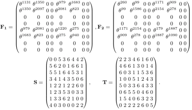
Definition 1. Let F = [fi,j] ∈ Mn×n Fqd

be the non-standard matrix representation of a HFE-shaped polynomial F ∈ Fqd[X₁, . . . , X_N]. We have n = N d, and the matrix F can be

divided in N ×N blocks of size d×d. We denote then by F∗d,k ∈ Mn×n Fqd

the matrix obtained from F by rotating the rows and columns of each d×d blocks from k positions and raising each components to the power qk. That is, if we denote by Fi,j the d×d block of F

located at position (i, j),0₆i, j < N, we have:

F∗d,k=



 

F∗_0,0k . . . F∗_0,Nk ₋₁

..

. ...

F∗_Nk₋_1,0. . .F∗_Nk₋_1,N₋₁ 

  .

The definition generalizes the one of F∗k. As in the univariate case the matrix F∗d,k indeed represents theqk-th power of a polynomial inFqd[X₁, . . . , X_N].

Proposition 5. Let F ∈ _F_qd[X₁, . . . , X_N] be a HFE-shaped polynomial and F = [f_i,j] ∈

M_n×n Fqd

be its non-standard matrix representation. F∗d,k is the non-standard matrix repre-sentation of Fqk_.

To prove Proposition 5, one can remark that the block Fi,j of the matrix F operates only on

the variablesXi+1 and Xj+1. To apply the Frobenius action to the whole polynomialF, it has

to be applied to each of these blocks, leading to the shape of F∗d,k. The precise proof can be found in Appendix B.

Thanks to Proposition 5, equation (4) can be generalized for multi-HFE. To this end, we propose a multivariate version of Lemma 1. Namely:

Lemma 2. Let MN,d ∈ Mn×n Fqd

be the matrix defined in Proposition 4. Let F1, . . . ,FN

be the non-standard symmetric matrices representing the secret polynomials F1, . . . , FN, and Fi∗d,k be the matrices defined in Definition 1. Finally, we consider the symmetric matrices

(H1, . . . ,Hn)∈ Mn×n(Fq) n

associated to the secret quadratic polynomials in the small field (h1, . . . , hn)∈ Fq[x1, . . . , xn]n, i.e. hi =xHixt for alli, 16i6n. It holds that:

(H1, . . . ,Hn) = MN,dF1∗d,0MtN,d, . . . ,MN,dF1∗d,d−1MtN,d, . . .

. . . ,MN,dFN∗d,0MtN,d, . . . ,MN,dFN∗d,d−1MtN,d

M−_N,d1.

Proof. The proof is very similar to the proof of Lemma 1. We start from the definition of the small field polynomialsh1, . . . , hn. For allv∈Fnq,

(h1(v), . . . , hn(v)) =ϕN F1 ϕ−N1(v)

, . . . , FN ϕ−N1(v)

.

Similarly, we need to express the above equation by matrix operations. We use then the definition of ϕN and its inverse using the matrixMN,d of Proposition 4, (h1(v), . . . , hn(v)) =

F₁q0(vMN,d), . . . , Fq d−1

1 (vMN,d), . . . , Fq

0

N (vMN,d), . . . , Fq d−1

N (vMN,d)

(15)

Recall from Proposition 5 that Fi∗d,j is the matrix representation of Fq

j

i , ∀i,1 6 i 6 N and

∀j,06j < d. We replace the polynomials by their matrix expression and we get for allv∈_Fn q:

(vH1vt, . . . , vHnvt) = vMN,dF1∗d,0MtN,dvt, . . . , vMN,dF1∗d,d−1MtN,dvt, . . .

. . . , vMN,dFN∗d,0MtN,dvt, . . . , vMN,dFN∗d,d−1MtN,dvt

M−_N,d1,

which concludes the proof. ut

Now, let U=T−1MN,d ∈ Mn×n Fqd

, W=S MN,d∈ Mn×n Fqd

and Fi(j)=WFi∗d,jWt,

withi, 16i6N, and j, 06j < d. We have the relation:

G(x) =T ◦ F ◦ S(x),

(g1(x), . . . , gn(x)) = h1(xS), . . . , hn(xS)

T, xG1xt, . . . , xGnxt

= xS H1Stxt, . . . , xS HnStxt

T, (G1, . . . ,Gn) = S H1St, . . . ,S HnSt

T.

Using Lemma 2:

(G1, . . . ,Gn) = S MN,dF1∗d,0MtN,dSt, . . . ,S MN,dF1∗d,d−1MtN,dSt, . . .

. . . ,S MN,dFN∗d,0MtN,dSt, . . . ,S MN,dFN∗d,d−1MtN,dSt

M−_N,d1 T. (6) Matrices Tand MN,d being invertible, we obtain:

(G1, . . . ,Gn) T−1MN,d= (F1(0), . . . ,F1(d−1), . . . ,FN(0), . . . ,FN(d−1)),

(G1, . . . ,Gn)U= (F1(0), . . . ,F1(d−1), . . . ,FN(0), . . . ,FN(d−1)). (7)

As in the univariate case, matricesU and W have a useful property.

Proposition 6. Let A= [ai,j]∈ Mn×n(Fq), and B = [bi,j] = A MN,d ∈ Mn×n Fqd

. For all i,06i < n, k,06k < N and j,06j < d, we have:

bi,k d+j =bq_{i,k d+((j}−1) modd).

That is, for each group of d columns, one column is obtained from the previous one using a Frobenius application. Each group ofdcolumns is defined by one of them, and consequently, the whole matrix is defined by N columns, one in each group.

The proof of Proposition 6 is similar to the proof of Proposition 3. The property comes from the fact that each group ofdcolumns is processed by a matrixMdleading to a similar property

as Proposition 3 for each group. The precise proof can be found in Appendix B.

To get the analogy with the MinRank in the univariate case, we remark that Fi∗d,0 = Fi.

By considering the (i d)-th columns ofU for alli,06i < N we have

n−1 X

k=0

uk,0Gk+1=WF1Wt, . . . ,

n−1 X

k=0

u_k,(N−1)dGk+1 =WFNWt. (8)

The following lemma allows to bind (8) to a MinRank problem.

Lemma 3. Let (F1, . . . , FN) ∈ (Fqd[X₁, . . . , X_N])N be polynomials having Multi-HFE shape.

For all k,1 ₆k₆N, let Fk ∈ Mn×n Fqd

be their non-standard symmetric matrix represen-tation. Let D be the degree of each polynomialFk and `=dlogqDe. For all k,16k6N

(16)

Furthermore, let

KN,d,` = 

    

0_d−`,`Id−`

0_d−`,d . . . 0d−`,d 0d−`,d . .. . .. ...

..

. . .. . .. 0d−`,d 0d−`,d . . . 0d−`,d

0_d₋_`,`I_d₋_`



    

∈ M_n−N `,n Fqd

where0d−`,` (resp.0d−`,d) is the zero matrix with (d−`)rows and`(resp. d) columns, andId−`

is the identity matrix with(d−`) rows and columns. Then, the rows of the matrix KN,d,` are a

basis of the left kernel of Fk with high probability and does not depend on the entries ofFk.

Proof. Each polynomial Fk has degree bounded by D, fork, 16k6N, thus each variableXi

has at most degree D, for all i,16i6N. The only non-zero entries of the matrix Fk are the

ones in the upper-left log_q(D) square of eachN×N block of size (d×d). Thus,Fkhas at most

N `non-zero rows and columns and has the following structure

Fk=



 

Ak0,0 . . . Ak0,N−1

..

. ...

AkN−1,0. . .AkN−1,N−1



 

where each blockAki,j is ad×dmatrix

Aki,j =



          

Ai,j_k,0,0 . . . Ai,j_k,0,` 0 . . . 0 ..

. ... ... ...

Ai,j_k,`,0 . . . Ai,j_k,`,` ... ... 0 . . . 0 ...

..

. . .. ...

0 . . . 0



          

fori, j, 06i, j < N. As the consequence, the rank of such matrixFk is at mostN `.

From the construction of KN,d,`, it is clear that KN,d,`Fk = 0. As KN,d,` has exactly

N(d−`) = (n−N `) linearly independent rows, if Rank(Fk) is exactly N `, which is the case

with high probability, then KN,d,` is a basis of the left kernel of Fk. ut

As in the univariate case, the problem of finding correct values forU turns to be a simulta-neous MinRank problem.

Theorem 3. For multi-HFE, recovering U =T−1MN,d ∈ Mn×n(Fqn) reduces to

simultane-ously solve N MinRank with k=n and r =Nlog_q(D) on the public matrices (G1, . . . ,Gn)∈

Mn×n(Fq)n. On the other hand, the solutions (i.e. the linear combinations) of each MinRank

are in Fqd.

Proof. TheN simultaneous MinRank come from (8). From Lemma 3, the rank ofFkis bounded

by r =Ndlog_q(D)e. Since W is invertible, the rank of WFkWt is equal to the rank ofFk for

all k,1 6 k 6 N. From Proposition 6, knowing one column in each of the N sequences of d columns in U is enough to recover the whole matrixU. This allows to conclude the proof. ut

(17)

4 About Equivalent Keys and Induced Degrees of Freedom

Two secret keys are equivalent if they lead to the the same public key. The subject has already been treated for the original HFE [42, 41, 43]. It has been shown thatn q2n(qn−1)2 equivalent keys exist for HFE. This phenomena is even amplified for multi-HFE. In this section, we exploit this fact.

Definition 2. Let (F∗,S,T) be a multi-HFE private key with parameters (q, N, d, D) ∈ N4.

We say that (F∗0,S0,T0) is an equivalent key if and only if F∗0 has HFE-shape, and

T0◦ϕN ◦ F∗0◦ϕ−_N1◦ S0 =G=T ◦ϕN ◦ F∗◦ϕ−_N1◦ S (same public key).

Wolf and Preneel [42, 43] introduced the notion of sustaining transformations which is a couple of affine transformations (A∗,B∗) such thatB∗◦ F∗◦ A∗ preserves the “shape” ofF∗. For HFE, the “big sustainer” (multiplication in the big field), the “additive sustainer” and the “Frobenius sustainer” keep the HFE-shape unchanged. In multi-HFE, multiplication keeps the HFE-shape. But, we also have any affine transformation on theN variables. Thus, the two first sustainers can be generalized as follows.

Proposition 7. Let (F∗,S,T) be a multi-HFE private key with parameters (q, N, d, D). For any invertible affine transformations(A∗,B∗)∈AffN(Fqd)×Aff_N(_F_qd), we setA=ϕ_N◦A∗◦ϕ−_N1

and B=ϕN◦ B∗◦ϕ−_N1. Then

B∗◦ F∗◦ A∗, A−1◦ S, T ◦ B−1

is an equivalent key.

Proof. First, we show that B∗◦ F∗◦ A∗ has HFE-shape. This is due to the fact that the only exponents occurring in a variableXi is a power ofq. The transformationA∗ mixes the variables

X1, . . . , XN by affine combinations. By linearity of the Frobenius, no other exponents can appear

and the system keeps its HFE-shape. Trivially, asB∗ only performs affine combinations of the polynomialsF1, . . . , FN the shape is also unchanged. To conclude, we notice that

G =T ◦ϕN ◦ F∗◦ϕ−_N1◦ S

G = T ◦ϕN◦ B∗−1◦ϕ−N1

◦ϕN ◦(B∗◦ F∗◦ A∗)◦ϕN−1◦ ϕN ◦ A∗−1◦ϕ−N1◦ S

G = T ◦ B−1

◦ϕN◦(B∗◦ F∗◦ A∗)◦ϕ−_N1◦ A−1◦ S

.

u t

The following proposition provides the structure of a transformation used in Proposition 7 in the linear case (it has to be slightly adapted in the affine case).

Proposition 8. Let A∗ = [ai,j]∈ MN×N Fqd

be the matrix associated to a linear transfor-mation A∗ _over ₍

Fqd)N. The transformation A∗ can be represented in the field _F_q as:

(18)

where MN,d ∈ Mn×n Fqd

is the matrix of Proposition 4 and Af∗ ∈ M_n×n Fqd

is a matrix composed of N ×N blocks of Frobenius powers of elements of A∗, i.e.

f A∗=

                

a0,0

aq₀_,₀

...

aqd₀_,₀−1 . . .

a0,N−1

aq₀_,N₋₁

...

aqd₀_,N−₋1₁ .. . ...

aN−1,0

aq_N−1,0 ...

aqd_N₋−₁1_,₀ . . .

aN−1,N−1

aq_N−1,N−1 ...

aqd_N₋−₁1_,N₋₁                 

Proof. Let (V1, . . . , VN)∈(Fqd)N. We set:

(Z1, . . . , ZN) =A∗(V1, . . . , VN) = N−1

X

i=0

ai,0Vi+1, . . . , N−1

X

i=0

ai,N−1Vi+1 !

.

According to Proposition 4, we need to compute the Frobenius images of (Z1, . . . , ZN) to split

it to the small field. For allk,06k < d, we have:

(Z₁qk, . . . , Z_Nqk) =

N−1 X

i=0

aq_i,0kV_i+1qk , . . . ,

N−1 X

i=0

aq_i,Nk ₋₁V_i+1qk

!

.

We notice thatZ_iqk is obtained only from theV_jqk’s for j, 16j 6N. This explains intuitively the shape of Af∗ We constructed the matrix Af∗ such that:

(V1, V1q, . . . , V qd−1

1 , . . . , VN, VNq, . . . , V qd−1

N )Af∗ = (Z₁, Z q 1, . . . , Z

qd−1

1 , . . . , ZN, ZNq, . . . , Z qd−1

N ).

(9) LetA∈ Mn×n(Fq) be the small field representation ofA∗, we now prove thatA=MN,dAf∗M−_N,d1 .

First, let (v1, . . . , vn) ∈ Fnq resp. (z1, . . . , zn) ∈ Fnq

be the small field representation of (V1, . . . , VN) (resp. (Z1, . . . , ZN)). It holds that

(v1, . . . , vn)A= (z1, . . . , zn).

From Proposition 4, we know that

(v1, . . . , vn)MN,d= (V1, V₁q, . . . , Vq d−1

1 , . . . , VN, V q N, . . . , V

qd−1

N ),

(z1, . . . , zn)MN,d= (Z1, Z1q, . . . , Z qd−1

1 , . . . , ZN, ZNq, . . . , Z qd−1

N ).

By replacing in (9), we get

(v1, . . . , vm)MN,dAf∗ = (z₁, . . . , z_m)M_N,d

(v1, . . . , vm)MN,dAf∗M−_N,d1 = (z₁, . . . , z_m).

Then,A=MN,dAf∗M_N,d−1 is the small field representation ofA∗. ut

(19)

Proposition 9. Let (F∗_,_S_,_T₎ _{be a multi-HFE private key with parameters} _{(q, N, d, D)}_∈

N4.

For all k,06k < d:

Frobk◦F∗◦Frobd-k, ϕN ◦Frobk◦ϕ_N−1◦ S, T ◦ϕN◦Frobd-k◦ϕ−_N1

is an equivalent key.

Proof. For any k,06k < d, the polynomials of

(Frobk◦F∗◦Frobd-k)(X1, . . . , XN) = F∗(Xq d−k

1 , . . . , X qd−k

N )

qk

have the same monomials as F∗(X1, . . . , XN) but their coefficients are raised to the power

of qk. This is explained in (2). As a consequence, if F∗(X1, . . . , XN) has HFE-shape, so is

(Frobk◦F∗◦Frobd-k)(X1, . . . , XN). In addition:

G=T ◦ϕN ◦ F∗◦ϕ−_N1◦ S

G= T ◦ϕN ◦Frobd-k◦ϕ−N1

◦ ϕN ◦Frobk◦F∗◦Frobd-k◦ϕ−N1

◦ ϕN ◦Frobk◦ϕ−N1◦ S

.

As the Frobenius application is linear inFq, the transformationsT ◦ϕN◦Frobd-k◦ϕ−N1 andϕN◦

Frobk◦ϕ−N1◦S remain affine. Finally, Frobk◦F∗◦Frobd-khas HFE-shape, proving Proposition 9.

u t

We introduce also the matrix representation of a Frobenius application.

Proposition 10. LetFrobk∈ Mn×n(Fq) be the matrix representing the linear transformation

ϕN◦Frobk◦ϕ−_N1 over Fq. Then

Frobk=MN,dPN,d,kM−_N,d1

where PN,d,k= Diag(Rd,k, . . . ,Rd,k

| {z }

N

) andRd,k is thed×dmatrix of ak positions left-rotation,

that is

Rd,k=

0k,d−k Ik Id−k 0d−k,k

.

Proof. Let (V1, . . . , VN)∈(Fqd)N. We set

Frobk(V1, . . . , VN) = (Vq k 1 , . . . , V

qk

N ) = (Z1, . . . , ZN).

In the big field, a leftk-rotation of (V, Vq, . . . , Vqd−1) is the application of Frobkto such vector.

Indeed, Frobk(V, Vq, . . . , Vq d−1

) = (Vqk, . . . , Vqd−1, V, . . . , Vqk−1). More generally, the matrix

PN,d,k makes this rotation on each N components in the big field. That is

(V₁q0, . . . , V₁qd−1, . . . , V_Nq0, . . . , V_Nqd−1)PN,d,k =

(V₁qk, . . . , V₁qd−1, V₁q0, . . . , V₁qk−1, . . . , V_Nqk, . . . , V_Nqd−1, V_Nq0, . . . , V_Nqk−1). We have then:

(V₁q0, . . . , V₁qd−1, . . . , V_Nq0, . . . , V_Nqd−1)PN,d,k= (Zq

0

1 , . . . , Z qd−1

1 , . . . , Z qk N, . . . , Z

qd−1

N ). (10)

As in the proof of Proposition 8, let (v1, . . . , vn)∈Fnq resp. (z1, . . . , zn)∈Fnq

be the small field representation of (V1, . . . , VN) (resp. (Z1, . . . , ZN)). According to Proposition 4, it holds that

(v1, . . . , vn)MN,d= (V1, V1q, . . . , V qd−1

1 , . . . , VN, VNq, . . . , V qd−1

N ),

(z1, . . . , zn)MN,d= (Z1, Z1q, . . . , Z qd−1

1 , . . . , ZN, Z_Nq, . . . , Zq d−1

(20)

By replacing in (10):

(v1, . . . , vm)MN,dPN,d,k= (z1, . . . , zm)MN,d

(v1, . . . , vm)MN,dPN,d,kM−N,d1 = (z1, . . . , zm).

Then,MN,dPN,d,kM−_N,d1 is indeed the small field representation of Frobk. ut

According to Proposition 9, we can derive (d−1) other equivalent keys from any valid private key. This refers to the so-called Frobenius sustainer of [42, 43]. To count the number of equivalent keys introduced by Proposition 7 and 9, we need to know how many different keys they generate. To do that, we will show that any equivalent key obtained from the Frobenius and affine sustainers has a unique representation.

Lemma 4. Let A∗ ∈AffN(Fqd). For all k, 0 6k < d, there exists A∗0 ∈AffN(Fqd) such that

Frobk◦A∗ =A∗0◦Frobk.

Proof. As Frobd-k◦Frobk is the identity, it holds that

Frobk◦A∗ = Frobk◦A∗◦Frobd-k◦Frobk.

Now we prove that A∗0 = Frobk◦A∗◦Frobd-k is an affine transformation. Let (X1, . . . , XN) ∈

(Fqd)N:

A∗0(X1, . . . , XN) = Frobk◦A∗◦Frobd-k(X1, . . . , XN) = Frobk◦A∗

X₁qd−k, . . . , X_Nqd−k

A∗0(X1, . . . , XN) = Frobk

PN−1

i=0 Ai,0Xq d−k

i+1 +A0, . . . , PN−1

i=0 Ai,N−1Xq d−k

i+1 +AN

A∗0(X1, . . . , XN) =

PN−1

i=0 Ai,0Xq d−k

i+1 +A0 qk

, . . . ,PN_i=0−1Ai,N−1Xq d−k

i+1 +AN qk

A∗0(X1, . . . , XN) =

PN−1 i=0 A

qk i,0X

qd i+1+A

qk N, . . . ,

PN−1 i=0 A

qk i,N−1X

qd i+1+A

qk N

A∗0(X1, . . . , XN) =

PN−1 i=0 A

qk

i,0Xi+1+A qk N, . . . ,

PN−1 i=0 A

qk

i,N−1Xi+1+A qk N

.

The transformation A∗0 is indeed an affine transformation with the same coefficients as A∗

raised to the powerqk. ut

Lemma 4 shows that the Frobenius and the affine transformation somehow commute. This will be useful to write uniquely an equivalent key.

Lemma 5. Let (A∗_,_A∗0₎_∈_Aff

N(Fqd)×Aff_N(_F_qd) be invertible affine transformations.

If Frobk◦A∗= Frobk0◦A∗0, for k, k0,06k, k0< d, then A∗0=A∗ and k0=k.

Proof. First, it is straightforward to see that if k=k0, then

Frobk◦A∗ = Frobk◦A∗0⇔Frobd-k◦Frobk◦A∗ = Frobd-k◦Frobk◦A∗0⇔ A∗ =A∗0.

Then, we have only to prove that Frobk◦A∗= Frobk0◦A∗0⇒k=k0. Assume for a contradiction

that there exists k and k0 such that Frobk◦A∗ = Frobk0◦A∗0 and k0 6=k. Then, we can write

k0 =k+`, with`6= 0:

Frobk◦A∗= Frobk0◦A∗0

Frobk◦A∗◦Frobd-k= Frobk+`◦A∗0◦Frobd-k

(21)

According to Lemma 4,Af∗ = Frob_k◦A ◦Frob_d-k andAf∗0 = Frob_k◦A∗0◦Frob_d-k are also affine

transformations. We write:

f

A∗_{= Frob}

`◦Af∗0.

As `6= 0, the transformation Frob`◦Af∗0 has degree q`. That is, each polynomial in the

repre-sentation of Frob`◦Af∗0has the form

PN i=1A

q` i X

q` i +A

q` 0

, withAi ∈Fqd. As Af∗0is invertible,

at least one term of degree q` is non-zero. Thus, Frob`◦Af∗0 cannot be equal to Af∗ which is an

affine transformation and has maximal degree 1. This proves that Frobk◦A∗ = Frobk0◦A∗0 ⇒

k=k0 andA∗ ₌_A∗0_. _u_t

Together with Lemma 4, Lemma 5 is used to derive a canonical representation of equivalent keys.

Theorem 4. Let (F∗,S,T) be a multi-HFE private key with parameters (q, N, d, D)∈N4. Let A∗,B∗ ∈ AffN(Fqd) be affine transformations in the big field and k,0 6 k < d be an integer.

Each Multi-HFE equivalent key (F0_,_S0_,_T0₎ _{obtained using Proposition 7 and 9 can be written} uniquely

F0 = Frobk◦B∗◦ F∗◦ A∗◦Frobd-k

S0 =ϕN◦Frobk◦A∗−1◦ϕ−N1◦ S

T0 =T ◦ϕN ◦ B∗−1◦Frobd-k◦ϕ−N1.

Proof. Let (F0_,_S0_,_T0_{) and (}_F_,_S_,_T_{) be equivalent keys. By hypothesis, a equivalent key has} been obtained by composition of several Frobenius and affine transformations. According to Lemma 4, the transformations can be reordered. Hence, any equivalent key can then be written as

F0= Frobk1◦ · · · ◦Frobkr◦B ∗

1◦ · · · ◦ Bn∗b◦ F

∗_{◦ A}∗

na ◦ · · · ◦ A

∗

1◦Frobd-kr◦ · · · ◦Frobd-k1

S0=ϕN ◦Frobk1◦ · · · ◦Frobkr◦A ∗−1

1 ◦ · · · ◦ A

∗−1 na ◦ϕ

−1 N ◦ S

T0=T ◦ϕN ◦ Bn∗−b1◦ · · · ◦ B

∗−1

1 ◦Frobd-kr◦ · · · ◦Frobd-k1◦ϕ −1 N .

The composition of two affine transformations is an affine transformation, and the composition of two Frobenius transformations is a Frobenius transformation. This can then be simplified as

F0 = Frobk◦B∗◦ F∗◦ A∗◦Frobd-k

S0 =ϕN◦Frobk◦A∗−1◦ϕ−N1◦ S

T0 =T ◦ϕN ◦ B∗−1◦Frobd-k◦ϕ−_N1.

To show the uniqueness of this representation, suppose that there exists A∗0,B∗0 ∈ AffN(Fqd)

and k0 ∈_N,06k < d leading to the same equivalent key. Then, by considering S0, we get:

ϕN ◦Frobk◦A∗−1◦ϕ−N1◦ S=ϕN ◦Frobk0◦A∗0−1◦ϕ−1

N ◦ S

Frobk◦A∗−1= Frobk0◦A∗0−1.

According to Lemma 5, this implies that k0 =k and A∗0−1 ₌_A∗−1_{. Similarly for} _T0_{, we show} thatB∗0−1 ₌_B∗−1_{, i.e. the representation is unique, proving the theorem.} _u_t

(22)

Theorem 5. Let (F∗_,_S_,_T₎ _{be a multi-HFE private key with parameters} _{(q, N, d, D)} _∈

N4.

There are exactly

d qdN

N−1 Y

i=0

(qdN−qd i)

!2

equivalent keys coming from affine transformations and Frobenius transformations.

Proof. According to Theorem 4, each equivalent key is uniquely defined by two invertible affine transformations (A∗_,_B∗₎_∈_Aff

N(Fqd)×Aff_N(_F_qd) and an integer k,06k < d. The number of

equivalent keys is the number of elements in

GLN(Fqd)×(_F_qd)N ×GL_N(_F_qd)×(_F_qd)N ×_Z/d_Z.

There are exactly QN_i=0−1 (qd)N−(qd)i

invertible matrices in M_N×N Fqd

. Thus, we obtain

the expected number of keys. ut

5 Weaknesses of HFE/multi-HFE Induced by Equivalent Keys

We show here that the high number of equivalent keys turns out to be a weakness for HFE/Multi-HFE schemes. For example, an interesting property of the MinRank arising in HFE/Multi-HFE/Multi-HFE/Multi-HFE is that the kernel of the matrices in (8) is independent of the equivalent key used up to Frobenius transforms. To show this property (Theorem 6), we first need to prove this property for a single private key.

Lemma 6. Let (F∗_,_S_,_T₎ _{be a multi-HFE private key with parameters} _{(q, N, d, D)} _∈

N4. We

denote by (G1, . . . ,Gn) ∈ (Mn×n(Fq))n the matrices associated to the public key G = T ◦

F ◦ S. Let S ∈ Mn×n(Fq) and T ∈ Mn×n(Fq) be the matrix representation of S and T,

respectively. Finally, let U = T−1MN,d = [ui,j]∈ Mn×n Fqd

, and K= ker(Pn_i=0−1ui,0Gi+1).

Then ∀t, k,0₆t < N, 0₆k < d,

ker

n−1 X

i=0

ui,t d+kGi+1

!

= Frobk(K) .

Proof. Lett,06t < N andk, 06k < d. Using equation (6) it holds thatPn−1

i=0 ui,t d+kGi+1=

SMN,dFt∗d,kMtN,dSt.AsS and MN,d are invertible, we have that

ker

n−1 X

i=0

ui,t d+kGi+1

!

= kerSMN,dFt∗d,k

ker

n−1 X

i=0

ui,t d+kGi+1

!

S MN,d= ker

Ft∗d,k

ker

n−1 X

i=0

ui,t d+kGi+1

!

= ker

Ft∗d,k

M−_N,d1 S−1.

Recall that`=dlog_q(D)e. With high probability, ker (Ft) = ker (F1) =KN,d,N `,∀t,16t6N

(see Lemma 3). From Definition 1, the non-zero columns of Ft∗d,k are the ones of Ft after

rotating the columns of each d×d blocks from k positions. Then, rotating accordingly the columns ofKN,d,N `leads to a basis of ker(Ft∗d,k). This rotation is exactly the one performed by

(23)

is a permutation matrix, its inverse is simplyPN,d,k(the rotation is done the other way). Finally

we obtain

kerPn_i=0−1ui,t d+kGi+1

=KN,d,N `PN,d,−kM−_N,d1 S−1

ker

Pn−1

i=0 ui,t d+kGi+1

=KN,d,N `

MN,dP−N,d,1 −k −1

S−1

=KN,d,N `(MN,dPN,d,k)−1S−1.

The matrix MN,dPN,d,k is obtained from MN,d by rotating the columns of each d×dblock to

the left. Due to the construction ofMN,d, this is equal to Frobk(MN,d). Then:

ker

Pn−1

i=0 ui,t d+kGi+1

=KN,d,N `Frobk(MN,d)−1S−1

=KN,d,N `Frobk

M−_N,d1 S−1.

As the coefficients of S and KN,d,N ` lie in the field Fq, this is equal to

ker

n−1 X

i=0

ui,t d+kGi+1

!

= Frobk

KN,d,N `M−_N,d1 S−1

.

Finally, asKN,d,N `= ker(F1) = ker(F1∗d,0), we conclude:

ker

n−1 X

i=0

ui,t d+kGi+1

!

= Frobk

ker(F1∗d,0)M−_N,d1S−1

= Frobk ker n−1 X

i=0

ui,0Gi+1

!!

ker

n−1 X

i=0

ui,t d+kGi+1

!

= Frobk(K).

This proves the lemma. ut

In other words, the kernel is unique up to Frobenius transformation. This property is used to prove the following theorem for any equivalent key.

Theorem 6. Let (F∗,S,T) and (F∗0,S0,T0) be equivalent multi-HFE private keys and

(G1, . . . ,Gn) ∈ (Mn×n(Fq))n be the matrices of their associated public key. Let (S, T) ∈

Mn×n(Fq)× Mn×n(Fq), and (S0,T0) ∈ Mn×n(Fq)× Mn×n(Fq) be the matrix

representa-tion of (S,T), and (S0,T0) respectively. Let U = T−1MN,d = [ui,j] ∈ Mn×n Fqd

, and

K = ker(Pn_i=0−1ui,0Gi+1). Similarly, let U0 = T0−1MN,d = [u0i,j] ∈ Mn×n Fqd

and K0 = ker(Pn_i=0−1u0_i,0Gi+1). Then ∃k, 06k < d, such that:

K0 = Frobk(K).

Proof. From Theorem 4, we can writeT0 =T ◦ϕN◦A∗−1◦Frobd-k◦ϕ−N1. Each of these application

has a matrix representation (see Proposition 4, 8 and 10). The matrix corresponding to T0 _is then T0 =MN,dPN,d,d−kAf∗−1M−_N,d1 T, where Af∗ has the shape of Proposition 8. Its inverse is

the matrixT0−1=T−1MN,dAf∗P−_N,d,d1 ₋_kM−_N,d1 . We have

(24)

LetAf∗P_N,d,k= [a_i,j]∈ M_n×n Fqd

, we have:

u0_i,j =

n−1 X

t=0

ui,tat,j,∀i, j,06i, j < n.

Due to the shape of Af∗ and P_N,d,k, a_t,j is non-zero if and only if t ≡ j−kmodd. Then, we

have u0_i,j =PN_t=0−1ui,t d+(j−kmodd)at d+(j−kmodd),j for all i, j,06i, j < n. Therefore n−1

X

i=0

u0_i,0Gi+1=

n−1 X

i=0 N−1

X

t=0

ui,t d+(−kmodd)at d+(−kmodd),0 !

Gi+1

=

N−1 X

t=0

at d+(−kmodd),0 n−1 X

i=0

ui,t d+(−kmodd)Gi+1

!

.

We denote by Γt,−k the matrix

Pn−1

i=0 ui,t d+(−kmodd)Gi+1

. One can see that the kernel of this matrix is the same for all t,06t < N. Indeed, according to Lemma 6:

ker (Γt,−k) = Frobt d+(-k mod d) mod d(K) = Frob-k mod d(K) ∀t,06t < N.

As

n−1 X

i=0

u0_i,0Gi+1=

N−1 X

t=0

at d+(−kmodd),0Γt,−k

is a linear combination of Γt,−k for t,0 6t < N, then ker (Γt,−k) ⊆ker

Pn−1

i=0 u0i,0Gi+1

. As

U0 is an equivalent key, there exists – according to (8) – a matrix W0 such that

n−1 X

i=0

u0_i,0Gi+1 =W0F1W0t,

so that the rank ofPn_i=0−1u0_i,0Gi+1 is Rank (F1).

Similarly from (7), we getΓt,−k=Pni=0−1ui,t d+(−kmodd)Gi+1 =W Ft+1∗d,−kWt, whereW

is invertible. As rotating rows and columns of a matrix does not change its rank, it holds that

Rank (Γt,−k) = Rank

Ft+1∗d,−k

= Rank (Ft+1) = Rank (F1) = Rank

n−1 X

i=0

u0_i,0Gi+1

!

.

Thus, we get ker (Γt,−k) = ker

Pn−1

i=0 u0i,0Gi+1

= K0. Finally,K0 = Frob-k mod d(K), proving

the theorem. ut

With Theorem 6, we know that the matrices of (8) have the same kernel (up to Frobenius transform), indenpendently on the equivalent key chosen.

Equivalent keys allow also to further slightly improve the MinRank attack. We consider an instance of HFE with parameters (q, N, d, D) ∈ _N4_{, and} _` ₌ _d_log_D_e_{. We have to solve the}

MinRank problem on the (n×n)-matricesG1, . . . ,Gn whose entries lie inFq with target rank

N `. Using the Kipnis-Shamir modeling described in [32, 26, 27], we have to solve the algebraic system of the (n(n−N `)) quadratic equations in (N `(n−N `) +n) variables given by the entries of the matrix



 

1 x1,1 . . . x1,N `

. .. .._. .._.

1xn−N `,1. . . xn−N `,N ` 

 ·

n X

i=1

λiGi

!