Generalised Random Binned Antenna Arrays
Giovanni Buonanno* and Raffaele Solimene
Abstract—In binned arrays, radiators are classically located according to a uniform probability distribution. By doing so, it has been shown that they have the same mean radiation pattern as totally random arrays (i.e., the ones for which the radiators’ positions are continuous independent and identically distributed random variables defined over the whole array aperture) but a lower variance. In this paper, we introduce a new class ofgeneralised binned arrays by generalising the rule for assigning the radiators’ positions. These new binned arrays, while maintaining the aforesaid advantage (in terms of the variance behaviour), allow to set the mean radiation pattern according to some design requirements. The achievable performance is estimated by measuring how much the radiation pattern deviates from the desired mean radiation pattern by resorting to the up-crossing theory. In particular, the study is developed for the case of symmetric arrays, which allows for easier maths. The paper includes an extensive numerical analysis which allows to check the developed theory. In particular, it focuses on the comparison between the generalised binned array and the totally random ones. A comparison with the nonuniform arrays coming from the density tapering approach is also presented. The latter appears natural in view of the new bins selection rule, which, as will be shown, is a sort of density-tapering in which the role of the reference current is played by the radiators’ position density distribution.
1. INTRODUCTION
Random arrays are those for which the positions of radiators are chosen according to some probabilistic law. This naturally leads to a nonuniform element arrangement (with probability one) which has a number of appealing features. Indeed, it is well known that nonuniform arrays are in principle free from grating-lobes and allow for large scan angles and/or wide frequency ranges; actually, the bandwidth-steerability product can be made much larger than for conventional equally-spaced arrays. Moreover, the number of radiators (especially for large aperture) can be reduced to a large extent (compared to the uniform arrangement) without significant degradation in the achievable resolution. This makes the problem of mutual coupling less severe. Finally, non-uniformly deploying the elements over the array aperture allows to control the side-lobe level without the need to taper the excitation currents. As a consequence, the amplifiers’ working points can be optimised and the costs connected to the need for solid-state T/R modules that work under arbitrary excitations and power outputs are reduced.
However, nonuniform arrays are much more difficult to analyse and synthesise than the uniform ones: this is because standard Fourier series tools cannot be employed. In particular, for random arrays the analysis and the synthesis must be pursued within the framework of stochastic processes and the achievable performance expressed in terms of probabilistic metrics.
Much of the work on random arrays dates back to the seminal paper by Lo [1] who was the first that systematically developed the theory for the case whereby radiators’ positions are continuous
i.i.d. random variables supported over the entire array aperture. This kind of random arrays is now
called totally random arrays (TRAs). Other different kinds of random arrays have also been proposed
Received 18 August 2017, Accepted 29 September 2017, Scheduled 8 October 2017
* Corresponding author: Giovanni Buonanno ([email protected]).
in literature (see [2] for a recent comparative study). Among them, we mention the binned arrays (BAs) [3] that are of particular interest for the present paper.
The characterisation of random arrays is usually achieved in terms of the mean array factor and its variance. The latter allows to foresee, for each observation angle, how much the array factor deviates from its average. A much more difficult question is the estimation of the side-lobe level (SLL). Actually, this is still an open problem since a rigorous and general procedure for SLL estimation has not been developed yet. This is due to the difficulty in determining the probability distribution of the array factor magnitude maximum in the side-lobe region (SLR). However, a number of approximate approaches have been proposed and found to be satisfactory [4–9]. Among them we mention the beam-pattern sampling approach, the up-crossings’ count and the extreme value theory. These approaches lead to tractable and relatively easy formulas only when the array factor is assumed weakly stationary. However, this assumption does not rigorously hold, especially for the SLR near the main beam. This problem is overcome, and the SLL estimated with better accuracy, if the radiators are symmetrically deployed (still according to a random law) with respect to the array aperture centre [10].
The synthesis problem amounts to selecting the array’s parameters in order to shape the radiation pattern so as to be “close” to the desired one (reference pattern). The goodness of the design process can then be estimated by measuring the mismatch between the reference and the obtained radiation patterns (design error) according to some common metric. This framework of course also applies to the case of random arrays. In particular, for the TRAs it is relatively easy to make the average radiation pattern close to the reference one. To this end, it is sufficient to choose the radiators’ position probability density function equal to the continuos current (supported over the array aperture) that gives the desired radiation pattern. Accordingly, the design error measures how much the random radiation pattern deviates from its average. Such an error can be estimated under theL2 norm by employing the Karhunen-Loeve expansion [1]. This however requires computing the eigenspectrum of the radiation pattern covariance function, which in general cannot be obtained in closed form. Moreover, different metrics like the design error magnitude could be of interest as well. Regardless of the metric one may want to adopt, for sure, a key role is played by the radiation pattern variance. One would like to have the variance as low as possible, for each observation angle, so that the random radiation pattern is close to the average one. In this regard, BAs are shown to be better than TRAs. More in detail, it was shown that, for the case of the radiators’ locations chosen according to a uniform distribution, BAs have a lower variance than TRAs. This is particularly true for the side-lobes close to the main beam. Hence, for that region the radiation pattern basically coincides to the average one. The point is that, due to the uniform distribution, the average pattern exhibits a sinc-like behaviour. Therefore, the question arising is to devise BAs which retain the afore mentioned variance behaviour but at the same time allow to freely choose the mean radiation pattern according to some design requirements.
The latter is just the main aim of this contribution. Herein, we develop a procedure that allows to obtain BAs which exhibit a desired mean radiation pattern and still have lower variance than TRAs. To this end, the probabilistic law for the elements’ allocation needs to be generalised: for this reason we address these new BAs as generalised BAs (GBAs). Remarkably, it is found that the new procedure for generating the GBAs is closely related to the density-tapering approach, which is a common deterministic way to synthesise nonuniform equally excited arrays [12, 13]. In particular, it is shown that the role of the continuos reference current in the density-tapering is here played by the radiators’ position probability density function.
In order to measure how much the radiation pattern deviates from the average one, we measure the mismatch (between the random radiation pattern and its average) magnitude. The latter is estimated by exploiting the up-crossing method upon assuming a Poisson distribution for the up-crossing process. Furthermore, the study focuses on the case of symmetric arrays which, as mentioned above, lead to more tractable maths.
2. BASICS ABOUT RANDOM ARRAYS
In this section, the basic theory concerning the Totally Random Arrays (TRAs) and the Binned Arrays (BAs) is briefly recalled in order to establish the framework and introduce the necessary notation.
2.1. Totally Random Arrays
Consider a linear array of equally-excited isotropic radiators arranged over a line of length L (in wavelength). The corresponding (normalised) array factor reads as
F(u) = 1
N
N
n=1
ej2πXnu =F(u) +jF(u) (1)
where
• N is the number of radiators;
• Xn is the position of the n-th radiator measured in wavelength;
• θandθ0are the observation and the steering angles, respectively, both measured from the broadside direction;
• u= sinθ−sinθ0. Though for a fixed steering angle the visible interval is [−1−sinθ0; 1−sinθ0], in the sequel the full scan range u∈[−2; 2] will be considered;
• F(u) and F(u) are the real and imaginary parts of the array factor.
If the positions {Xn}Nn=1 are assigned according to a probabilistic rule, then the array factor is a stochastic process. Accordingly, the probability theory is needed for describing/studying the array radiation properties. In this framework, the mean patter φ(u) = E[F(u)] and the variance
E[|F(u)|2]− |φ(u)|2 are generally rather easy to compute. For TRAs the positions {X
n}s are assumed independent and identically distributed (i.i.d.), then the mean and the variance of the array factor read as [1]
φ(u) =
L/2
−L/2f(X)e
j2πXudX (2)
and
σ2(u) =1− |φ(u)| 2
N (3)
where f(X) is the commonpdf of the radiators’ positions. Note that f(X) is just supported over the array aperture [−L/2, L/2]. At this juncture, it is useful to highlight an obvious fact that descends from Eq. (2). It can be noted that the relationship between f(X) and φ(u) is the same as that connects a continuous current and its radiation pattern. Therefore, as mentioned above, the mean array factor can be easily set by choosing the{Xn}s’pdf which has the desired Fuourier transform. Of course, this does not assure that the array factor fulfils the synthesis requirements because it can deviate from its mean patter according to the variance behaviour. Also, one is not free to choose f(x) arbitrarily because it needs to be a probability density function.
The array factor is also commonly characterised in terms of its magnitudeA(u) =|F(u)|. Although herein we do not dwell on this aspect, it is however important to recall the basics aspects because they are relevant to the error computation which is shown subsequently. Determining the distribution of
A(u) requires finding the cumulative distribution (cdf) P(A(u) < ξ). This is in general a hard task. However, it is somehow simplified when the number of radiators is large. In this case, the Central Limit Theorem [11] allows to consider F and F to be jointly normal [1]. Moreover, if f(X) is even (as it is commonly assumed) [1] then the imaginary part of the mean pattern φ(u) = 0 and
F(u) and F(u) become uncorrelated (and hence independent) for each value of u. In other words,
denoting the normal distribution. Accordingly, the cumulative distribution function of the array factor magnitude is
P(A(u)< ξ) =
e−
[FR−φ(u)]2 2σ2R(u) +
FI2
2σ2I(u)
2πσR(u)σI(u) dFRdFI
|F(u)|<ξ
(4)
Equation (4) is a generalised non central chi-square distribution with two degrees of freedom. As well known, it cannot be computed in closed form even though some approximations can be employed to simplify the calculation [14].
2.2. Binned Arrays
For BAs, the following generation rule is used for determining the radiators’ positions
Xn=−L2 + (n−1)L
N +Yn; n= 1,2, . . . , N (5)
where {Yn}Nn=1 are independent continuous random variables defined over the interval [0, L/N]. This type of arrays are known as Binned Arrays because the array aperture is divided into equal non-overlapping intervals, called bins, and in each of them a single radiator is located. The statistical properties of this kind of random arrays was studied in [3] where the positions{Yn}Nn=1were assumed to be uniformly distributed over [0, L/N] (i.e., f(Yn) =U(0, L/N)∀n). For such a case, the mean pattern
φBA(u) and the variance σBA2 (u) are given by
φBA(u) = N1
N
n=1
Eej2πXnu= 1
L L/2
−L/2e
j2πXudX =φ
U(u) (6)
and
σ2BA(u) = 1−E[e
j2πY u]2
N =σ
2
U(u/N) (7)
Here,φU(u) andσU2(u) are the corresponding mean and variance of the array factor of a TRA when in Eqs. (2) and (3) the common pdf of the elements’ positions is assumed uniform over [−L/2, L/2] (i.e.,
U(−L/2, L/2)). First, it is observed that for both types of arrays the maximum possible aperture is
L. This entails that the achievable resolution (in terms of the width of the main beam) is basically the same. Also, Eq. (6) shows that theBAs have the same mean array factor as theT RAs. Therefore, for this simple case (i.e., {Yn} uniformly distributed) a clear connection (as for TRAs) exists between the mean pattern and the positions’ pdf. Finally, the BAs are in general better than TRAs because the variance increases more slowly as umoves away from the main beam region (see (7)). This means that the BA factor is “closer” (statistically) to its mean factor over a larger range (in u) than the T RAs. However, the array factor magnitude characterisation becomes more complicated. Indeed, the Central Limit Theorem still allows to consider a Gaussian probability distribution for the array factor. However, looking at the cross-covariance between F(u) and F(u), which is given by
Cov[F, F;u] = N12
N
n=1
E[sin(4πXnu)]
2 −E[cos(2πXnu)]E[sin(2πXnu)]
(8)
it can be observed that F(u) and F(u) are in general not independent. Hence, while computing (4), the correlation coefficient must be taken into account.
3. GENERALISED BINNED ARRAYS
In the previous section, we have shown that BAs and TRAs have the same mean array factor, but BAs are somehow better because the variance increases more slowly while moving away from the main beam region. This result has been established according to the Hendricks’s work [3] by assuming the radiators’ positions asi.i.d. uniform random variables. Unfortunately, for such a case the mean radiation pattern is bound to be a sinc-like function. In this section, we aim at generalising the probabilistic law for generating the radiators’ positions in order to have BAs whose mean pattern can be set according to some requirement; at the same time the advantage in terms of the variance behaviour must be retained. Let us start by reinterpreting the assigning rule in Eq, (5). Denote as ˜xn = −L2 + (n−1)NL
for n = 1,2, . . . , N + 1. Hence, the array aperture results partitioned into the N equal bins
[˜x1,x˜2]∪[˜x2,x˜3] ∪. . . ∪ [˜xn−1,x˜n]∪ . . . ∪[˜xN,x˜N+1]. In each bin the element position is chosen
according to a uniform distribution. In particular, for the n-th bin Xn ∼ U[˜xn,x˜n+1]. Now consider
f(X) =U(−L/2, L/2). It then results that thepdfs of the BA elements are related to f(X) as follows
f(Xn) =N f(X) Π
⎛ ⎜ ⎝X−
˜
xn+ ˜xn+1
2 ˜
xn+1−x˜n
⎞ ⎟
⎠ (9)
where Π[(X−a)/b] is the window function centred in awith extension equal to b. Hence, f(Xn)s are obtained fromf(X) through a partitioning and rescaling procedure, and this, as shown above, assures that φBA(u) = φU(u). This result strictly holds for the case of uniform distribution and needs to be generalised for a more generalf(X). In particular, as we are going to show, a nonuniformf(X) entails a nonuniform allocation of the ˜xn.
Say φD(u) the desired mean radiation pattern and let fD(X) the pdf supported over [−L/2, L/2] whose Fourier transform returns φD(u). Define the f(Xn) as in Eq. (9). It then follows that
φGBA(u) =φD(u), that is
φGBA(u) = N1
N
n=1
Eej2πXnu= 1
N
N
n=1
L/2
−L/2f(Xn)e
j2πXnudX n
= 1
N
N
n=1
x˜n
˜ xn−1
N fD(X)ej2πXudX =
L/2
−L/2fD(X)e
j2πXudX =φ
D(u) (10)
as long as
L/2
−L/2f(Xn)dX =
x˜n
˜ xn−1
N fD(X)dX = 1 (11)
Indeed, Eq. (11) assures thatf(Xn)s are normalised, and hence that they are actually probability density functions. Also, it provides the law needed to choose the ˜xn. In particular, consider the cumulative function
FD(x) =
x
−L/2fD(X)dX (12)
for which of course holds that FD(−L/2) = 0 and FD(L/2) = 1. Then, Eq. (11) entails dividing the range ofFD(x) intoN intervals of size 1/N. Accordingly, theN + 1 ˜xn are determined as
˜
x1=−L/2 =FD−1(0); ˜x2 =FD−1(1/N); . . . x˜n+1=FD−1(n/N);. . .x˜N+1 =FD−1(1) =L/2 (13) so that the array aperture results divided intoN non-equal intervals [˜x1,x˜2]∪[˜x2,x˜3]. . .∪[˜xn−1,x˜n]. . .∪ [˜xN,x˜N+1] and within each of them the radiator’s position is fixed according to Eq. (9).
It is interesting to remark that the partition rule in Eq. (13) is basically the same as the one used for the synthesis of deterministic nonuniform arrays according to the density-tapering approach proposed by Doyle in [12] and then discussed by Skolnik in [13]. In particular, here the roles of the positive and real continuous reference current and the so-calledcumulative distribution current are respectively played byfD(X) andFD(x).
(i) fix fD(X) according to the desired mean radiation pattern;
(ii) determine the ˜xns according to the distribution functionFD(x) as shown in Eq. (13); (iii) finally choose theXn pdf usingfD(X) in Eq. (9).
As remarked, this procedure allows to have the desired mean radiation pattern. As to the variance, it yields
σ2GBA(u) = E[|FGBA(u)|2]− |φGBA(u)|2
= 1 N2 N n=1 N m=1
E[ej2πXnue−j2πXmu]− 1
N2 N n=1 N m=1
E[ej2πXnu]E[e−j2πXmu]
= 1 N − 1 N2 N n=1
|E[ej2πXnu]|2 = 1
N − N n=1
x˜n
˜ xn−1
fD(X)ej2πXudX
2
(14)
from which, recalling Eq. (3), it can easily be seen that the variance is lower than the one corresponding to a TRA whenfD(X) is used for generating the elements’ positions.
Also for GBAs one can still say that both the real and imaginary parts of the array factorFGBA(u) are asymptotically normal, but the same difficulties mentioned above persist while determining the distribution of the array factor magnitude. To mitigate this inconvenient, we propose to introduce the symmetry requirement in order to exploit the simplifications arising.
3.1. Symmetric Generalised Binned Antenna Arrays
First, the desired pdf fD(X) is assumed even with respect to the centre of the array aperture. This assumption guarantees that the bins, provided by Eq. (13), are symmetric as well. However, this does not entail that the resulting array is already symmetric. To this end, we need to enforce that for each radiator located atXn>0 a symmetric radiator is put at−Xn. In essence, one starts fromfD(X) and determines the bins only for positive x. In this case, ˜x1 = 0 and ˜xN/2+1=L/2. Then, in each of these bins Xn is selected. Finally, the array is completed by putting elements also at −Xn. In particular, in the sequel we consider only arrays with an even number of radiators. This is done for the sake of simplicity and has no practical impact on arrays consisting of a large number of elements.
The array factor of a symmetricGBA can be written as
FGBAs(u) = 2
N
N/2
n=1
cos(2πXnu) (15)
whereas the mean and variance are yielded by
φGBAs(u) = E[FGBAs(u)] = 2
N
N/2
n=1
E[cos(2πXnu)] = 2
N
N/2
n=1
x˜n+1
˜ xn
f(Xn) cos(2πXu)dX
= 2
N
N/2
n=1
x˜n+1
˜ xn
N fD(X) cos(2πXu)dX = 2
L/2
0
fD(X) cos(2πXu)dX =φD(u) (16)
and
σ2GBAs(u) = 1
N + 2 N2 N/2 n=1
E[cos(4πXnu)]− 4
N2
N/2
n=1
E2[cos(2πXnu)]
= 1
N[1 +φD(2u)]−
4
N2
N/2
n=1
E2[cos(2πXnu)] (17)
If the number of elements is sufficiently large, by the Central Limit Theorem, the array factor pdf
can be considered normal, FGBAs(u) ∼ N[φGBAs(u), σ2
asymmetric case, the cdf of the array factor magnitude, AGBAs(u) = |FGBAs(u)|, is obtained in closed form without any approximations. Indeed, sayξ ∈R+, it yields [10]
P{AGBAs(u)≤ξ} = P{−ξ≤FGBAs(u)≤ξ}=
ξ
−ξ
1
2πσGBA2 s(u)
e−
[FGBAs−φGBAs(u)]2 2σGBA2 s(u)
dFGBAs
= Q
−ξ+φGBAs(u) σGBA2 s(u)
−Q
ξ−φGBAs(u)
σGBA2 s(u)
(18)
where Q(x) = (1/√2π)x∞e−ξ2/2dξ is related to the so-called error function that can be obtained in closed form with a small error making use of the analytical approximation in [15], which holds for positive arguments. A further clear advantage with respect to the asymmetric arrays is that also the mean and variance of the magnitude array factor can be evaluated in closed form [10]. Indeed, the array factor magnitude density can be easily evaluated after a simple transformation as
f(AGBAs, u) = 1
2πσ2 GBAs(u)
⎧ ⎨ ⎩e
−[AGBAs−φGBAs(u)]2 2σ2GBAs(u) +
e−
[AGBAs+φGBAs(u)]2 2σ2GBAs(u)
⎫ ⎬
⎭ (19)
and then
φAGBAs(u) = E[AGBAs(u)]
= φGBAs(u)
Q
−φGBAs(u) σGBAs(u)
−Q
φGBAs(u)
σGBAs(u)
+
2
πσGBAs(u)e
−φ2GBAs(u)
2σ2GBAs(u) (20)
σ2AGBAs(u) = σ2GBAs(u) +φ2GBAs(u)−φ2AGBAs(u) (21)
3.2. Error Estimation
As stated at the beginning of this paper, we are also interested in estimating how the radiation pattern deviates from φD(u). To this end, we obviously need the statistic characterisation of the error process magnitude |(u)|= |FGBAs(u)−φD(u)|. The latter is a simple task if we note that the error process coincides with the magnitude of the centred array pattern process, i.e., (u) ∼ N[0, σ2GBAs(u)]
Accordingly, under the assumption of symmetric radiators’ positions, the distribution P(|(u)|< ξ) is easily found by considering a zero mean pattern in the results reported in the previous section. However, this would only regard a “punctual” (i.e., for each separated u) characterisation of the error. Indeed, to globally estimate the error the supremum of ε= maxu∈[0,2]{|(u)|} must be studied, where only the interval [0,2] has been considered in virtue of the evenness of the radiation pattern. Basically, this entails finding the following distribution
P{ε≤ξ}=P{|(u)| ≤ξ ∀u∈[0,2]} (22)
Finding theεdistribution is clearly linked to the estimation of the side-lobes of the centred radiation pattern. As such, it is a hard and in general an open problem. However, a number of approximate methods have been proposed in the literature. In this paper we employ the up-crossing approach. In detail, say ξ the level with respect to which the number of up-crossings has to be estimated and say
Nξ the random variable that counts how many times|(u)| up-crosses ξ (i.e., crosses ξ with a positive slope). Accordingly, ε can be estimated by finding the threshold ξ for which the probability of no crossing is one. This is equivalent to estimating P(Nξ ≥ 1), i.e., that at least there is one up-cross. This task is greatly simplified if we content to find an upper bound forP(Nξ≥1) (resp. a lower bound forP(Nξ= 0)). To this end,E[Nξ] can be exploited. Indeed, according to Rice’s formula [16]
E[Nξ] =
2
0
du
∞
0
||f||||(ξ,||;u)d|| (23)
wheref||||(||,||;u) is the jointpdf between the error and its derivative|| = d||du. Note that Eq. (23)
uncorrelated and Gaussian hence their joint pdf f can be readily obtained by multiplying the marginal distributions. Then,f||||(||,||;u) is obtained from f
(, ,
, ;u). However, in general |(u)| is not stationary and the computation of E[Nξ] requires performing a multidimensional numerical integration. In the case of symmetric random arrays this matter is greatly simplified [10]. In fact, since(u) is a real process, determining the up-crossings of|(u)|is equivalent to simultaneous study the up-crosses of (u) and ˜(u) = −(u) for the given level ξ > 0. Since (u) and (u), and of course ˜(u) and ˜(u), are jointly Gaussian, then the mean number of up-crossings can be written as
E{Nξ} =
2
0
du +∞
0
f(ξ, , u)d+
2
0
du +∞
0 ˜
f˜˜(ξ,˜, u)d˜
= 2
2
0
du
∞
0
e
− 1
2[1−ρ2(u)]
ξ2 σ2(u)−
2ρ(u)ξ σ(u)σ(u)+
2
σ2(u)
2πσ(u)σ(u) 1−ρ2(u)
d (24)
Note that σ2(u) = σ2GBAs(u), whereas σ2(u) is the variance of (u) and ρ(u) = E[(u), (u)]/(σ(u)σ(u)) is the correlation coefficient that can be computed as shown in [10].
Once E[Nξ] has been computed the Markov inequality can be invoked to get
P{Nξ≥1} ≤ E[Nξ] (25)
or equivalently
P{Nξ= 0} ≥ 1−E[Nξ] (26)
Of course, Eq. (25) or (26) is meaningful only when E[Nξ]≤1. Accordingly, ε can be estimated as the value ofξ for whichE[Nξ] is sufficiently lower than 1.
A direct estimation of P{ε ≤ ξ} can still be obtained in terms of E[Nξ] if the occurrence of the up-crossing points is assumed to be a random point Poisson process [8]. In this case it can be shown that
P{ε≤ξ} ≈e−E[Nξ] (27)
Eventually, the latter is theεestimation that will be used in the sequel.
4. NUMERICAL RESULTS
In this section, some numerical results are shown in order to assess the theory presented in the previous sections. To this end, two different kinds of desired radiation patterns are considered: the first one is the cosine distribution
fD1(X) = π
2L cos
π X L
(28)
which provides the following mean radiation pattern
φD1(u) =
cos(πLu) 2 + 4Lu +
cos(πLu)
2−4Lu (29)
the second one is a Taylor distribution of parameters ¯n= 80 and SLL= 0.1
fD2(X) =
⎡ ⎣1 + 2
¯ n−1
p=1
φD2(p/L)
⎤ ⎦
L (30)
with
A = cosh
−1(1/SLL)
π ; (31)
σ = ¯n
to which the following mean radiation pattern corresponds
φD2(u) =
sin(πLu)
πLu
¯ n−1%
n=1
&
1−
u
un
2'
¯ n−%1
n=1
&
1−
u n/L
2' (33)
with the nulls at
un=±σ A
2+ (n−1/2)2
L (34)
SayFGBAi(u) andFT RAi(u), withi= 1,2, the generalised BA and TRA random radiation patterns
corresponding to the mentionedpdfs. Also, both classes of arrays are assumed symmetric (in the sense explained above) even though the superscript s (as in Section 3.1) has been skipped for simplicity of notation. Finally, the wavelength λis fixed at 1 m.
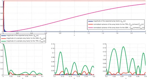
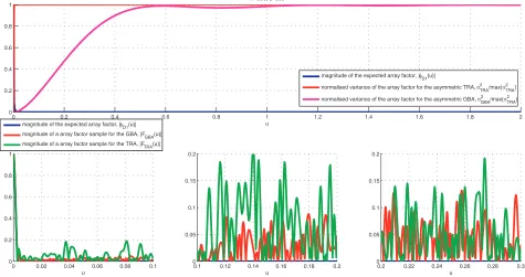
In Figs. 1–3 and 4–6, we start by showing the variance behaviour and the effect it has on the radiation patterns for the distributionfD1andfD2, respectively. The number of radiators has been fixed atN = 200 but the case where they are deployed over array apertures of different sizes is considered. In particular, for the three considered cases, the average distance between two consecutive radiators, defined asL/N, is 0.5λ,λand 2.5λ. In each figure, the top diagram reports the magnitude of the mean array factor (blue line), i.e., the desired |φDi(u)|, and the normalised, with respect to maxu∈[0,2]{σ2T RA(u)}, variances behaviours; the red line is forσ2
T RA(u) whereas the magenta line refers toσ2GBA(u). As can be seen, the advantages of the binned arrays shown in [3] are also confirmed for the case at hand where the positions of the elements do not have uniformpdf distribution within each subinterval. More in detail, as expected,σGBA2 (u) increases in a much slower way thanσ2T RA(u), even though as the element average
0 0.2 0.4 0.6 0.8 1 1.2 1.4 1.6 1.8 2
0 0.2 0.4 0.6 0.8
1 N=200, L=100
u
0 0.02 0.04 0.06 0.08 0.1 0
0.2 0.4 0.6 0.8 1
u
0.1 0.12 0.14 0.16 0.18 0.2 0
0.02 0.04 0.06 0.08 0.1 0.12 0.14
u
0.2 0.22 0.24 0.26 0.28 0.3 0
0.02 0.04 0.06 0.08 0.1 0.12 0.14 0.16
u magnitude of the expected array factor, |φD1(u)|
normalised variance of the array factor for the TRA, σTRA2 (u)/max{σ TRA 2 (u)}
normalised variance of the array factor for the GBA, σGBA2 (u)/max{σ TRA 2 (u)}
magnitude of the expected array factor, |φD1(u)| magnitude of a sample array factor for the GBA, |F
GBA(u)|
magnitude of a sample array factor for the TRA, |F
TRA(u)|
0 0.2 0.4 0.6 0.8 1 1.2 1.4 1.6 1.8 2 0
0.2 0.4 0.6 0.8
1 N=200, L=200
u
0 0.02 0.04 0.06 0.08 0.1 0
0.2 0.4 0.6 0.8 1
u
0.1 0.12 0.14 0.16 0.18 0.2 0
0.02 0.04 0.06 0.08 0.1 0.12 0.14 0.16
u
0.2 0.22 0.24 0.26 0.28 0.3 0
0.05 0.1 0.15 0.2 0.25
u magnitude of the expected array factor, |φD1(u)|
normalised variance of the array factor for the TRA, σTRA2 (u)/max{σ TRA 2 (u)}
normalised variance of the array factor for the GBA, σGBA2 (u)/max{σ TRA 2 (u)}
magnitude of the expected array factor, |φD1(u)| magnitude of a array factor sample for the GBA, |F
GBA(u)|
magnitude of a array factor sample for the TRA, |F
TRA(u)|
Figure 2. The case of cosine distribution. The number of radiators isN = 200 and are deployed over an aperture of L = 200. The top diagram reports the desired mean radiation pattern along with the normalised (to max{σT RA2 }) variance behaviours, whereas the bottom ones illustrate the comparison betweenφD1(u) and GBA and TRA sample (realisation) patterns.
0 0.2 0.4 0.6 0.8 1 1.2 1.4 1.6 1.8 2
0 0.2 0.4 0.6 0.8 1
N=200, L=500
u
0 0.02 0.04 0.06 0.08 0.1 0
0.2 0.4 0.6 0.8 1
u
0.1 0.12 0.14 0.16 0.18 0.2 0
0.05 0.1 0.15 0.2
u
0.2 0.22 0.24 0.26 0.28 0.3 0
0.05 0.1 0.15 0.2
u magnitude of the expected array factor, |φD1(u)|
normalised variance of the array factor for the asymmetric TRA, σTRA2 /max{σ TRA 2 }
normalised variance of the array factor for the asymmetric GBA, σGBA 2 /max{σ
TRA 2 }
magnitude of the expected array factor, |φD1(u)|
magnitude of a array factor sample for the GBA, |F
GBA(u)|
magnitude of a array factor sample for the TRA, |F
TRA(u)|
0 0.2 0.4 0.6 0.8 1 1.2 1.4 1.6 1.8 2 0
0.2 0.4 0.6 0.8 1
N=200, L=100
u
0 0.02 0.04 0.06 0.08 0.1 0
0.2 0.4 0.6 0.8 1
u
0.1 0.12 0.14 0.16 0.18 0.2 0
0.05 0.1 0.15 0.2 0.25
u
0.2 0.22 0.24 0.26 0.28 0.3 0
0.05 0.1 0.15 0.2 0.25
u magnitude of the expected array factor, |φD2(u)|
normalised variance of the array factor for the TRA, σTRA 2 (u)/max{
σTRA 2 (u)}
normalised variance of the array factor for the GBA, σGBA 2 (u)/max{
σTRA 2 (u)}
magnitude of the expected array factor, |φD2(u)|
magnitude of a array factor sample for the GBA, |FGBA(u)|
magnitude of a array factor sample for the TRA, |FTRA(u)|
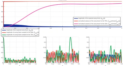
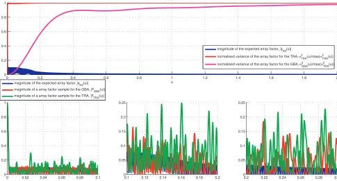
Figure 4. The case of Taylor distribution. The number of radiators is N = 200 and are deployed over an aperture of L = 100. The top diagram reports the desired mean radiation pattern along with the normalised (to max{σ2
T RA}) variance behaviours, whereas the bottom ones illustrate the comparison betweenφD2(u) and GBA and TRA sample (realisation) patterns.
0 0.2 0.4 0.6 0.8 1 1.2 1.4 1.6 1.8 2
0 0.2 0.4 0.6 0.8 1
N=200, L=200
u
0 0.02 0.04 0.06 0.08 0.1
0 0.2 0.4 0.6 0.8 1
u
0.1 0.12 0.14 0.16 0.18 0.2
0 0.05 0.1 0.15 0.2 0.25
u
0.2 0.22 0.24 0.26 0.28 0.3
0 0.05 0.1 0.15 0.2 0.25
u
magnitude of the expected array factor, |φD2(u)|
normalised variance of the array factor for the TRA, σTRA2 (u)/max{σ
TRA 2
(u)}
normalised variance of the array factor for the GBA, σGBA2 (u)/max{σ
TRA 2 (u)}
magnitude of the expected array factor, |φD2(u)|
magnitude of a array factor sample for the GBA, |FGBA(u)|
magnitude of a array factor sample for the TRA, |FTRA(u)|
0 0.2 0.4 0.6 0.8 1 1.2 1.4 1.6 1.8 2 0
0.2 0.4 0.6 0.8 1
N=200, L=500
u
0 0.02 0.04 0.06 0.08 0.1 0
0.2 0.4 0.6 0.8 1
u
0.2 0.22 0.24 0.26 0.28 0.3 0
0.05 0.1 0.15 0.2 0.25
u 0.1 0.12 0.14 0.16 0.18 0.2
0 0.05 0.1 0.15 0.2 0.25
u
magnitude of the expected array factor, |φD2(u)|
normalised variance of the array factor for the TRA, σTRA2 (u)/max{σ TRA 2 (u)}
normalised variance of the array factor for the GBA, σGBA2 (u)/max{σ TRA 2 (u)}
magnitude of the expected array factor, |φD2(u)| magnitude of a array factor sample for the GBA, |F
GBA(u)|
magnitude of a array factor sample for the TRA, |F
TRA(u)|
Figure 6. The case of Taylor distribution. The number of radiators is N = 200 and are deployed over an aperture of L = 500. The top diagram reports the desired mean radiation pattern along with the normalised (to max{σ2
T RA}) variance behaviours, whereas the bottom ones illustrate the comparison betweenφD2(u) and GBA and TRA sample (realisation) patterns.
spacing increases, both variances reach their maximum value more quickly. For theT RAs this can be easily explained since a larger aperture corrisponds to a narrower first-null beam-width (see Eq. (3)). A similar reasoning also applies for the GBAs since the larger the array aperture the larger the bin extensions and hence the first-null beam-width of each terms in the summation of Eq. (14). In any case, even by increasing the average spacing between antenna elements the growth of variance ofGBAs
becomes faster, and the relative advantage over theT RAs is maintained, because the bins are always smaller than the whole aperture, although for both array types the region of randomness†, within the visible space, becomes larger.
The bottom diagrams reported in each figure instead show a comparison between the desired mean radiation pattern (blue lines) and the corresponding|FGBAi|(red lines) and|FT RAi|(green lines)
realisations. As can be seen, while for TRAs the radiation pattern manifests a random structure nearly immediately, the|FGBAi|s follow well the desired radiation pattern in the near main beam zone, and in
general stay closer to φDi(u) than the TRAs.
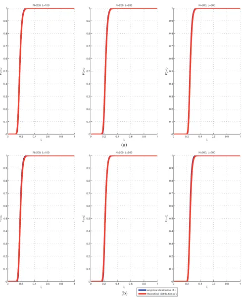
We now move to assess the validity of Eq. (27) for estimating the errorε. In particular, in Fig. 7, the error probability distribution returned by Eq. (27) is compared with empirical results obtained via a Monte Carlo procedure. In particular, for the Monte Carlo analysis, the array factors were sampled with a step equal toλ/(10L), that is five times finer than the Nyquist step corresponding to the bandwidth of the array square magnitudes. Moreover, each empirical distribution was built by running (generating) 10000 trials (for each case). As can be seen, the obtained results are amazing for both the considered
pdfs. Hence, Eq. (27) can be safely used to estimate the maximum error as the one for which the probability is one.
Finally, as mentioned above, in view of the similarity between the bin generation rule and the density-tapering, it makes sense to compare the error returned by the GBAs and the Doyle-Skonlink synthesis. Say FDT(u) the radiation pattern arising from the density-tapering procedure. As above,
0 0.2 0.4 0.6 0.8 1 0 0.1 0.2 0.3 0.4 0.5 0.6 0.7 0.8 0.9 1 N=200, L=100 ξ P{ ε < ξ }
0 0.2 0.4 0.6 0.8 1 0 0.1 0.2 0.3 0.4 0.5 0.6 0.7 0.8 0.9 1 N=200, L=200 ξ P{ ε < ξ }
0 0.2 0.4 0.6 0.8 1 0 0.1 0.2 0.3 0.4 0.5 0.6 0.7 0.8 0.9 1 N=200, L=500 ξ P{ ε < ξ } (a)
0 0.2 0.4 0.6 0.8 1 0 0.1 0.2 0.3 0.4 0.5 0.6 0.7 0.8 0.9 1 N=200, L=100 ξ P{ ε < ξ }
0 0.2 0.4 0.6 0.8 1 0 0.1 0.2 0.3 0.4 0.5 0.6 0.7 0.8 0.9 1 ξ P{ ε < ξ } N=200, L=200
0 0.2 0.4 0.6 0.8 1 0 0.1 0.2 0.3 0.4 0.5 0.6 0.7 0.8 0.9 1 ξ P{ ε < ξ } N=200, L=500
empirical distribution of ε
theoretical distribution of ε
(b)
Figure 7. Illustrating the validity of (27). Panel (a) reports the comparison between the theoretical ε
we define the error as δ = maxu∈[0,2]|FDT i(u)−φDi(u)|. In particular, we compare the two methods by reporting the probability that the GBAs give a lower error than FDT(u), that is P{ε ≤δ}. Some results corresponding to the configurations already exploited in the previous examples are shown in the following tables. These results clearly show that as the average distance between the elements increases, with high probability, the GBAs are better than the density-tapering arrays. In this regard, it is worth remarking that the GBAs error measure can be considered as a tool for a priori estimating the performance achievable by the synthesis of density-tapered arrays.
Table 1. Cosine density function.
N L δ P{ε≤δ}
200 100 0.1007 0 200 200 0.3070 0.9954
200 500 0.3121 0.9851
Table 2. Taylor density function.
N L δ P{ε≤δ}
200 100 0.1283 0
200 200 0.2664 0.9596
200 500 0.2687 0.8478
5. CONCLUSIONS
In this paper, we introduce a method for obtaining binned arrays which allows to use any desired pdf
for the radiators’ positions. We name this class of binned arrays “generalised binned arrays” since they actually expand the repertoire of this kind of arrays and generalise the classical binned array theory [3] which implicitly assumes a uniform pdf. In particular, one can make the mean radiation pattern coincident to the one corresponding to a generic real and positive current defined over the whole array aperture. This was possible by noticing that the bins generation rule coincides to the bins density procedure when the chosen pdf is equal to the reference current.
This result sheds new light on the possibility offered by the binned arrays. Indeed, through the GBAs one can shape the mean radiation pattern (which does not necessarily need to be a sinc-like function anymore) according to some design constraints. At the same time GBAs retain the advantage, over the totally random ones, in terms of the variance behaviour. The latter entails that the corresponding random array radiation pattern is closer to the average one over a larger region around the main beam than TRAs are, and in this sense GBAs always outperform TRAs.
For the sake of convenience, the study has been thoroughly developed for the case of symmetric arrays. More in detail, the maximum of the mismatch between the random pattern and the desired mean one has been estimated in closed form by resorting to the up-crossing theory. Finally, GBAs also appear advantageous compared to the density-tapered arrays when the average spacing between radiators is greater than λ/2. Finally, we want to emphasise the fact that since the generalised binned arrays and density-tapered arrays are tied by sharing the same bins, the framework used to analyze the former can also be used for a priori analysis of the latter, even before any synthesis procedures.
ACKNOWLEDGMENT
REFERENCES
1. Lo, Y. T., “A mathematical theory of antenna arrays with randomly spaced elements,”IEEE Trans. Antennas and Propagation, Vol. 12, 257–268, 1964.
2. Buonanno, G. and R. Solimene, “Comparing different schemes for random arrays,” Progress In Electromagnetics Research B, Vol. 71, 107–118, 2016.
3. Hendricks, W. J., “The totally random versus the bin approach for random arrays,” IEEE Trans. Antennas and Propagation, Vol. 39, 1757–1762, 1991.
4. Agrawal, V. D. and Y. T. Lo, “Distribution of sidelobe level in random arrays,”Proc. IEEE, Vol. 57, No. 10, 1764–1765, 1969.
5. Agrawal, V. and Y. T. Lo, “Mutual coupling in the phased arrays of randomly spaced antennas,” IEEE Trans. Antennas and Propagation, Vol. 20, 288–295, May 1972.
6. Agrawal, V., “Mutual coupling in phased arrays of randomly spaced antennas,” Ph.D. dissertation, University of Illinois at Urbana-Champaign, Jan. 1971.
7. Donvito, M. B. and S. A. Kassam, “Characterization of the random array peak sidelobe,” IEEE Trans. Antennas and Propagation, Vol. 27, 379–385, May 1979.
8. Krishnamurthy, S., D. Bliss, and V. Tarokh, “Sidelobe level distribution computation for antenna arrays with arbitrary element distributions,” 2011 Conference Record of the Forty Fifth Asilomar Conference on Signals, System and Computers (ASILOMAR), 2045–2050, Nov. 2011.
9. Krishnamurthy, S., D. Bliss, C. Richmond, and V. Tarokh, “Peak sidelobe level gumbel distribution for arrays of randomly placed antennas,” 2015 IEEE Radar Conference (RadarCon), 1671–1676, 2015.
10. Buonanno, G. and R. Solimene, “Large linear random symmetric arrays,” Progress In Electromagnetics Research M, Vol. 52, 67–77, 2016.
11. Papoulis, A. and S. U. Pillai,Probability, Random Variables and Stochastic Processes, 4th Edition, McGraw Hill, 2002.
12. Doyle, W., “On approximating linear array factor,” RAND Corp. Mem RM-3530-PR, 1963. 13. Skolnik, M. I., “Ch. nonuniform arrays,”Antenna Theory, R. E. Collin and F. Zucker, Eds., Pt. I,
McGraw-Hill, New York, 1969.
14. Lo, Y. T., “Aperiodic arrays,” Antenna Handbook, Y. T. Lo, S. W. Lee, Antenna Theory, Vol. 2, Chapter 14, Chapman & Hall, 1993.
15. Couch, L. W.,Digital and Analog Communication Systems, 6th Edition, Prentice Hall, 2001. 16. Cram´er, H. and M. R. Leadbetter, Stationary and Related Stochastic Processes: Sample Function