The Rebound Attack and Subspace
Distinguishers: Application to Whirlpool
Mario Lamberger1, Florian Mendel1, Christian Rechberger2, Vincent Rijmen1,2, and Martin Schl¨affer1
1 Institute for Applied Information Processing and Communications
Graz University of Technology, Inffeldgasse 16a, A–8010 Graz, Austria.
2 Dept. of Electrical Engineering ESAT/COSIC, K.U.Leuven,
and Interdisciplinary Institute for BroadBand Technology (IBBT), Kasteelpark Arenberg 10, B–3001 Heverlee, Belgium.
Abstract. We introduce the rebound attack as a variant of differen-tial cryptanalysis on hash functions and apply it to the hash function Whirlpool, standardized by ISO/IEC. We give attacks on reduced vari-ants of the Whirlpool hash function and the Whirlpool compression func-tion. Next, we introduce the subspace problems as generalizations of near-collision resistance. Finally, we present distinguishers based on the rebound attack, that apply to the full compression function of Whirlpool and the underlying block cipherW.
Keywords:hash functions, cryptanalysis, near-collision, distinguisher
1
Introduction
A cryptographic hash function H maps a message m of arbitrary length to a fixed-length hash valueh. Informally, a cryptographic hash function has to fulfill the following three classical security requirements: preimage resistance, second preimage resistance and collision resistance. The resistance of a hash function to these attacks depends in the first place on the length N of the hash value. Regardless of how a hash function is designed, an adversary will always be able to find preimages or second preimages after trying out about 2N different messages. Finding collisions requires a much smaller number of trials: about 2N/2 due to the birthday paradox. A function is said to achieveideal security if these bounds are guaranteed.
In this paper, we provide a detailed analysis of the hash function Whirlpool. This hash function is based on a dedicated block cipherW, which was designed according to the Wide Trail design strategy. It is the only hash function stan-dardized by ISO/IEC (since 2000) [1] that does not follow the MD4 design strategy.
One contribution of this paper is to give an in-depth account of therebound attack, as a variant of differential cryptanalysis heavily optimized to the crypt-analysis of hash functions, and at the same time as a high-level model for hash function cryptanalysis. The rebound attack can be used to construct various types of collisions. Thus far, it has been very successful on designs that copy the simple byte-oriented structure of AES.
Our second contribution is the introduction and definition of the subspace problems, as a natural extension and formalization of the near-collision require-ment. We give bounds for the difficulty of the subspace problems in the generic (or ideal) case. Finally, we show subspace distinguishers for the full compression function of Whirlpool, thereby demonstrating the first deviation from the ideal model of this function.
Parts of this work appeared before in abridged form in [26,31]. New in this paper are the extended descriptions of the rebound attacks, proper definitions for the two subspace problems and the proofs on the lower bounds of the query complexities of these problems in the generic case.
Organization. In Section 2, we describe the rebound attack. We introduce
two subspace problems in Section 3 and give bounds for their difficulty in the generic case. We describe the hash function Whirlpool in Section 4. We start by discussing classical attacks on reduced variants of the Whirlpool hash function in Section 5. Next we discuss classical attacks on reduced variants of the Whirlpool compression function in Section 6. Finally, we give subspace distinguishers for the compression function in Section 7, and for the underlying block cipherW in Section 8. We conclude in Section 9.
2
The Rebound Attack
The rebound attack was proposed by Mendel et al. in [31] for the cryptanalysis of AES-based hash functions. It is a differential attack, using several new techniques to improve upon existing results.
2.1 Differential Cryptanalysis of Block Ciphers
cryptographic primitive, is called acharacteristic, or sometimesdifferential path
ortrail. A pair that exhibits the differences of the characteristic, is called aright pair. The fraction of right pairs over all input pairs, possibly averaged over all keys (when the primitive is keyed), is called theprobability of the trail.
Truncated differentials were proposed by Knudsen as a tool in block cipher cryptanalysis [22]. While in a standard differential attack, the full difference between two inputs/outputs is considered, in the case of truncated differen-tials, the differences are only partially determined, e.g. for every byte, one only checks if there is a difference or not. Truncated differentials have been applied by Peyrin [39] in the cryptanalysis of the hash function Grindahl [24].
2.2 Differential Cryptanalysis of Hash Functions
Rijmen and Preneel described differential attacks on hash functions based on a reduced variant of DES, with 15 instead of 16 rounds [40]. Also the attacks on MD4 by Dobbertin [13], on SHA by Chabaud and Joux [8], and on MD4, RIPEMD and SHA-1 by Wang et al. [43,44] are differential attacks. Most re-cently, Khovratovich et al. analyzed the security of AES-based hash functions with respect to collision resistance [5,21].
If we apply differential cryptanalysis to a hash function, a collision for the hash function corresponds to a right pair for a trail through that hash function, with output difference zero. Similarly, a near-collision corresponds to a right pair for a trail with an output difference of low Hamming weight. It follows that differential cryptanalysis of hash functions is intuitively very similar to differential cryptanalysis of block ciphers. However, there are also important differences between these two cases, as can be observed with the rebound attack in the next section.
In the case of block ciphers, an adversary that wants to find a right pair can usually do little better than simply trying out pairs. The needed effort is proportional to the inverse of the probability of the trail. Since hash functions do not have a secret key, an adversary can do better than that. In principle, an adversary could simply write out the equations that determine whether a pair is a right pair and solve them. In practice, these equations are highly nonlinear and difficult to solve. However, it is often possible to determine some of the message bits, thereby increasing the probability that a random guess for the remaining part of the solution will be correct. Typically, the equations arising from the first steps of the hash function are easier to solve, because they do not yet depend on all message words. These techniques are known in the literature under the name
message modification techniques [44].
Hence, a (near-)collision attack on a hash function, that is based on differ-ential cryptanalysis, can be described as follows.
1. Find a trail with a high probability.
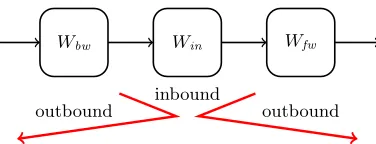
Wbw Win Wfw
inbound
outbound outbound
Fig. 1. A schematic view of the rebound attack. The attack consists of an
in-bound and two outin-bound phases.
2.3 The Rebound Attack
The rebound attack consists of two phases, called inbound and outbound phase, as shown in Figure 1. According to these phases, the compression function, internal block cipher or permutation of a hash function is split into three sub-parts. LetWbe a block cipher, then we getW =Wfw◦Win◦Wbw. Hence, the part of the inbound phase is placed in the middle of the cipher and the two parts of the outbound phase are placed next to the inbound part. In the outbound phase, two high-probability (truncated) differential trails are constructed, which are then connected in the inbound phase. Similar to message modification, the freedom in the message, key-inputs or (internal) state variables is used to efficiently fulfill many conditions of a differential trail.
The idea of placing the most expensive part of the differential trail in the middle was previously used in the cryptanalysis of the compression function of MD5 [12] and the hash function Tiger [20,30,33]. Also, inside-out techniques as used in the rebound attack, were invented by Wagner as an application of second order differentials in the cryptanalysis of block ciphers in the Boomerang attack [42].
Constructing a Trail. As in all differential attacks we first need to construct
a “good” (truncated) differential trail. A good trail used for a rebound attack should have a high probability in the outbound phases and can have a rather low probability in the inbound phase. Two properties are important here: First, the system of equations that determine whether a pair follows the differential trail in the inbound phase, should be under-determined. Then, many solutions (starting points for the outbound phase) can be found efficiently by using guess-and-determine strategies. Second, the outbound phases need to have high probability in the outward direction.
Inbound Phase. The inbound part of a trail is defined such that the
high probability. Hence, also a differential trail with a high Hamming weight (and hence a low probability) can be used in the inbound phase.
Outbound Phase. In the outbound phase, we verify whether the solutions of
the inbound phase also follow the differential trail in the outbound parts. Note that in the outbound phase, there are usually only a few or no free variables left. Hence, a solution of the inbound phase will lead to a solution of the out-bound phase with a probability significantly smaller than 1. Therefore, we aim for narrow (truncated) differential trails in the outbound parts, which can be fulfilled with a probability as high as possible (in the outward directions). The advantage of using an inbound phase in the middle and two outbound phases at the beginning and end is that one can construct differential trails with a higher probability in the outbound phase.
Using more Inbound Phases. Sometimes, not all available freedom is used
in the rebound attack. This is usually the case if some parts of the (internal) state or the input of the key schedule is not needed to find a solution in the inbound phase [26,28]. In these cases, the attack can often be extended to more rounds by having one or more independent inbound phases and then connect the solutions of the inbound phases. Note that this is usually not a trivial task. However, it is possible in the compression function attacks on Whirlpool using the freedom of the round keys as shown in Section 6.
3
The Subspace Problem
In [37], NIST requires that a good hash function should fulfill several properties. Along with the well known security notions of collision resistance and (second) preimage resistance, NIST also requires that any K-bit hash function specified by taking a fixed subset of the N output bits should possess the same security assertions as the original function. Of course, an attacker can choose theK-bit subset specifically to allow a limited number of precomputed message digests to collide, but once the subset has been chosen, finding additional violations of the above notions should again have the generic complexity.
From a practical application point of view, this requirement makes a lot of sense when we want to guarantee security in cases where the output space of the hash function is reduced by means of a simple truncation. However, instead of simply truncating the hash function output, the application developer might also choose to split the output string in two halves and xor them together [18,19]. This method is almost as simple as truncation, but the security requirement on the hash function becomes now that it should be difficult to construct two messagesm, m∗ such that
H(m)⊕H(m∗) =z, (1)
could formulate as generalized requirement that for any linear transformationL, it should be hard to find two inputsm,m∗ such that
L(H(m∗)⊕H(m)) = 0. (2)
Clearly, the adversary should not be able to choose L, because for all m, m∗, it is trivial to find an Lsatisfying 2. On the other hand, if we require that the adversary can find suitable m, m∗ for any arbitrarily selectedL, or for a large
subset of them, then, it may become too difficult to find an adversary for many intuitively bad hash function designs. In order to get out of this dilemma, we propose to generalize a bit further by defining the following problem.
Subspace Problem 1 (Subspace Problem for One-Way Functions)
When given a one-way functionf mapping toFN2 , try to findtinput pairs(ai, a∗i)
such that the corresponding output differencesf(ai)⊕f(a∗i)belong to a subspace Vout⊂FN2 withdim(Vout)≤nfor somen≤N.
HereF2=GF(2) denotes the finite field of order 2.
If f is a hash or compression function, then solving Subspace Problem 1 should behard, whennis significantly smaller thanN, sayn≤ N
2. Otherwise, the hash function has a certificational weakness. We show in Section 6 how Subspace Problem 1 can be solved when f is the compression function of Whirlpool, but first we discuss what we mean when we state that Subspace Problem 1 should behard.
3.1 On the Hardness of Subspace Problem 1
In this section, we investigate how difficult it is to solve Subspace Problem 1 without using knowledge of the internals of the function f. We measure the difficulty by counting the number of queries that need to be made to the oracle. We bound the query complexity and ignore all other computations, memory accesses etc.
Let us now assume that an adversary is makingQ 2N/2 queries to the function f. We thus get K ≤ Q2
differences (∈ FN2) coming from these Q queries. For given nand t > n, we now want to calculate the probability that among theK corresponding output differencesf(ai)⊕f(a∗i), we have tvectors (output differences) that belong to a subspaceVout⊆FN2 with dim(Vout)≤n.
We will need the following fact about matrices over finite fields. LetE(t, N, d) denote the number of t×N matrices overF2 that have rank equal to d. Then, it is well known [14,27] that
E(t, N, d) = d−1 Y
i=0
(2N−2i)·(2t−2i) 2d−2i =
d−1 Y
i=0
(2N −2i)· t
d
2
, (3)
where dt
Proposition 1 Let n, t, N ∈ N be given such that t ≥ N > n. We assume a set ofK vectors (output differences) chosen uniformly at random from FN
2. Let Pr(K, t, N, n) denote the probability that t of these K vectors span a subspace
Vout⊆FN2 withdim(Vout)≤n. Then, we have
Pr(K, t, N, n)≤ K
t
2−t·N n X
d=0
E(t, N, d). (4)
This probability is upper bounded by
Pr(K, t, N, n)≤ √1 2πt
Ke
t t
2−(N−n)(t−n)+(n+1). (5)
For the proof of Proposition 1, we will first need two lemmas.
Lemma 1. Let t, N, n∈N be such thatt≥N > n. Then,
E(t, N, n)≤ n X
d=0
E(t, N, d)≤2·E(t, N, n).
Proof. The first inequality is trivial. The second one is equivalent to
n−1 X
d=0
E(t, N, d)≤E(t, N, n).
and can be proven by induction overn. Forn= 1,E(t, N,0)≤E(t, N,1) which is easily seen to be true. So let us assume that
n−2 X
d=0
E(t, N, d)≤E(t, N, n−1)
holds. To prove the statement, we add E(t, N, n−1) to both sides. If we can show that 2E(t, N, n−1)≤E(t, N, n), we are done. From (3) we derive
2E(t, N, n−1) = 2 n−2
Y
i=0
(2N −2i)·
t n−1
2 ,
E(t, N, n) = n−1
Y
i=0
(2N −2i)· t n 2 .
Sincet≥N > n, we have
2
t n−1
2
≤(2N −2n−1)
t n 2 .
The proof follows from the fact that
t
n
2 =2
t−n+1−1 2n−1
t
n−1
2 .
Lemma 2. Let t, N, n∈N be such thatt≥N > n. Then,
(2t−2i)·(2N−2i) 2n−2i ≤
(2t−2j)·(2N −2j) 2n−2j
holds for all 0≤i < j≤n−1.
Proof. We show this by proving that for givenA > B > C >0 the function
f(x) = (A−x)(B−x) C−x
has always a positive derivative f0(x) on the interval x∈[0, C/2]. Elementary calculus shows that the derivative off(x) is
f0(x) = (A−C)(B−C) (C−x)2 −1,
from which we easily see that the conditionf0(x)>0 is satisfied if
(A−C)(B−C)>(C−x)2
holds. The right side is smaller thanC2which means that the statement is equal to
AB > C(A+B)
If we substituteA= 2t, B= 2N, C= 2n we see that the last inequality holds in
our setting and we are done. ut
Now, we are in the position to prove Proposition 1.
Proof (of Proposition 1).Remember that E(t, N, d) was defined as the number of t×N matrices overF2 that have rank equal tod. Computing Pr(K, t, N, n) exactly would require the application of the inclusion-exclusion principle since the ranks of the Kt
considered subspaces are not independent. Therefore, we take (4) as an upper bound for the probability Pr(K, t, N, n).
Simplifying the upper bound consists of two steps. Bounding the binomial coefficient and bounding the rest. Based on Lemma 1 and 2 we can estimate the second part of the probability Pr(K, t, N, n) by
2−t·N n X
d=1
E(t, N, d)≤2−t·N·2·E(t, N, n)
≤2−t·N+1
(2t−2n−1)·(2N −2n−1) 2n−2n−1
n
≤2−t·N+12n−1·2t−(n−1)·2N−(n−1)
n
= 2−(t−n)(N−n)+(n+1)
For the binomial coefficient Kt
we combine the simple estimate Kt
≤Kt/t!
with the following inequality based on Stirling’s formula [41]:
√ 2πtt+
1 2e−t+
1
12t+1 < t!<√2πtt+ 1 2e−t+
1
12t (7)
From this we get
K
t
≤√1
2πt K·e
t t
. (8)
Putting together (6) and (8) proves the proposition. ut As a corollary, we can give a lower bound for the number of random vectors needed to fulfill the conditions of the proposition with a certain probability.
Corollary 1 For a given probabilitypand givenN, n, tas in Proposition 1, the
number K of random vectors needed to contain t vectors that span a subspace
Vout⊆FN2 withdim(Vout)≤nwith probabilitypis lower bounded by
K≥ t e
p√2πt 1 t 2
(N−n)(t−n)−(n+1)
t . (9)
Proof. Equation (9) follows immediately from (5). ut
Corollary 2 For a given probability p and given N, n, t as in Proposition 1,
the and the number of queries Q to f needed to produce t vectors that span a subspaceVout⊆FN2 withdim(Vout)≤nwith probabilitypis lower bounded by
Q≥ r
2t e
p√2πt
1 2t
2
(N−n)(t−n)−(n+1)
2t . (10)
Proof. (10) follows from settingK≤ Q 2
=Q(Q−1)/2 in (9). ut
3.2 The Permutation Case
This section is devoted to the study of the Subspace Problem in the case where the function f is replaced by a permutation π. In the case of a permutation, one can define adversaries that are allowed to make forward queries (i.e. to π) and backward queries (i.e. toπ−1). Clearly, backward queries render Subspace Problem 1 trivial, since the adversary can fix pairs with output differences in Vout and simply ask the backward queries. Therefore, if we want to define a meaningful subspace problem, we have to formulate additionally constraints on the inputs.
Subspace Problem 2 (Subspace Problem for Permutations)
When given a permutation πmapping fromFN
2 to FN2, try to findt input pairs (ai, a∗i)such thatai⊕a∗i belong to a subspace Vin⊆FN2 withdim(Vin)≤mand
the corresponding output differencesπ(ai)⊕π(a∗i)belong to a subspaceVout ⊆FN2
One can distinguish between two types of adversaries: the non-adaptive ad-versary and the adaptive adad-versary. While in the adaptive setting, the adad-versary can use the results of previous queries to select subsequent inputs for the next queries, the adversary has to decide on the inputs for the queries on before-hand in the non-adaptive setting. In all of the following, we will only consider non-adaptive adversaries.
Now we want to give a bound on the success probability of the adversary for solving Subspace Problem 2 when it is given oracle access to a permutation π and its inverseπ−1. The adversary is allowed to make at mostQqueries in total toπandπ−1. Denote byQ1the number of queries that the adversary makes to π, and byQ2=Q−Q1 the number of queries made toπ−1.
Let us now start with theQ1 queries toπ. It is easy to see that by choosing the inputs in a sub-vector space of dimensionm we get K1 ≤ Q21
input pairs (ai, a∗i) and hence input differences ai⊕a∗i belonging to a subspace Vin⊆FN2 with dim(Vin)≤m. This approach obviously allows a maximum of 2mqueries. In order to be able to make more queries we take the subsequent inputs to be in a translate of Vin, that is, we take ai, a∗i ∈ u+Vin = {u+v|v ∈ Vin} where u6∈Vin. We can repeat this several times for differentu6∈Vin. So if we setQ1=q1·2m+r1 andr1<2m,q1≥0, by makingQ1 queries toπ we get
K1=q1·
2m 2
+
r1
2
(11)
input differencesai⊕a∗i belonging to a vector spaceVinwith dim(Vin)≤m. Analogously to Proposition 1 we will first consider the case of differences. Note that the Q1 queries to π are chosen such that the resulting K1 input differences lie in a subspace Vin whereas the corresponding output differences can be assumed uniformly distributed inFN2. In a similar way, theQ2queries to π−1result inK
2output differences in a spaceVoutwhere again the corresponding input differences are uniformly distributed. So in total we have K1+K2 pairs of input and output differences.
Proposition 2 Let n, m, t, N ∈N be given such that t≥N >2n and m≤n.
We assume a set ofK:=K1+K2difference pairs{(a1, b1), . . . ,(aK, bK)}where bi is uniformly distributed inFN2 andai is taken from some subspaceVin⊆FN2
for i = 1, . . . , K1 and where ai is uniformly distributed in FN2 and bi is taken
from some subspace Vout ⊆FN2 fori= 1, . . . , K2.
LetPr(K, t, N, m, n)denote the probability thatt of theseK difference pairs are such that the input differences span a subspaceVin0 ⊆FN2 withdim(Vin0 )≤m
and the output differences span a subspace Vout0 ⊆ FN2 with dim(Vout0 ) ≤ n,
simultaneously. Then, we have
Pr(K, t, N, m, n)≤ t
X
t1=0 K
1 t1
K
2 t−t1
2−t·N
m X
i=0
E(t−t1, N, i) n X
j=0
E(t1, N, j).
This probability can be upper bounded by
Pr(K, t, N, m, n)≤ √1 2πt
Ke
t t
2−(N−n)(t−2n)+2(n+1). (13)
Proof. The K =K1+K2 difference pairs described in the proposition can be seen as elements (ai, bi)∈FN2 ×F
N
2 , where in the firstK1 pairs, theai’s can be chosen, and in the last K2 the bi’s can be chosen by an adversary. In order to have the highest possible probability for the event in the proposition these values would always be chosen to be a fixed differencea6= 0 andb6= 0. The 0 difference is impossible when keeping in mind that they come from queries, so choosing identical differences leads to the smallest dimension for the difference vectors that can be controlled. So whenevertof theKdifference pairs are selected, and say t1 are taken from the first K1 pairs, andt−t1 from the second K2 pairs, we can start to upper bound the sought probability by (12). This is because the probability that t of these input differences span a space of dimension ≤m is upper bounded by
2−(t−t1)N m X
i=0
E(t−t1, N, i). (14)
Here we use thatt1input differences are identical and we apply Proposition 1 to the remaining t−t1 input differences, where we count the F2-matrices of rank ≤m. The sum in (14) is an overestimation since when the fixed input difference ais not in the span of the remainingt−t1differences, we would only be allowed to take the matrices of rank≤m−1 into account. Analogously, we get for the output differences
2−t1N n X
i=0
E(t1, N, i),
and since both conditions have to be satisfied simultaneously, we end up with (12).
To further bound (12) we proceed as follows. Without loss of generality, we assume thatm≤nand obtain
t X
t1=0 K
1 t1
K
2 t−t1
2−tN
n X
i=0
E(t−t1, N, i) n X
j=0
E(t1, N, j)
as an upper bound for the probability. Using Lemma 3 we can simplify the last sum to
K
t
2−tN+2E(2t, N, n)2
where we used
t X
t1=0 K
1 t1
K
2 t−t1
=
K 1+K2
t
.
Lemma 3. Let t, N, n ∈ N be such that t ≥ N > 2n and t1 ∈ {0,1, . . . , t}.
Then,
n X
i=0
E(t−t1, N, i) n X
j=0
E(t1, N, j)≤4E(2t, N, n)2. (15)
Proof. We first consider the case wheret1 ∈ {n, n+ 1, . . . , t−n}. This implies that both t1 and t−t1 are greater or equal than n. In this case, we can use Lemma 1 to estimate both sums and we get
n X
i=0
E(t−t1, N, i) n X
j=0
E(t1, N, j)≤4E(t−t1, N, n)E(t1, N, n).
The productE(t−t1, N, n)E(t1, N, n) can be written as n−1
Y
i=0
(2N−2i)2·(2t−t1−2i)·(2t1−2i) (2n−2i)2 .
From this and the fact that (2t−t1 −2i)·(2t1 −2i) ≤ (2t/2−2i)2 holds for
i∈ {0, . . . , n−1}follows the statement of the lemma fort1∈ {n, n+1, . . . , t−n}.
The caset1∈ {0,1, . . . , n−1}, respectivelyt1∈ {t−n+1, . . . , t}, is symmetric, so without loss of generality, we only consider the first case. Then, the estimate of Lemma 1 applied to (15) results in
n X
i=0
E(t−t1, N, i) t1 X
j=0
E(t1, N, j)≤4E(t−t1, N, n)E(t1, N, t1).
We can show
E(t−t1, N, n)E(t1, N, t1)≤E(t2, N, n)2 by splitting the statement into two inequalities:
E(t−t1, N, n)E(t1, N, t1)≤E(t−n, N, n)E(n, N, n) (16) E(t−n, N, n)E(n, N, n)≤E(t
2, N, n)
2 (17)
Here, (16) can be deduced with similar arguments as Lemma 2. To show (17) we look atE(t−n, N, n)E(n, N, n)E(t/2, N, n)−2and observe that
n−1 Y
i=0
(2t−n−2i)(2n−2i) (2t/2−2i)2 =
n−1 Y
i=0
2t−2t−n+i−2n+i+ 22i 2t−2t/2+i+1+ 22i ≤1,
since because of t > 2n, every term in the product is smaller or equal than 1. This proves the lemma in the case t1 ∈ {0,1, . . . , n−1}, respectively t1 ∈
{t−n+ 1, . . . , t}. ut
Corollary 3 Under the preliminaries stated in Proposition 2, the numberK of difference pairs such that simultaneously, the input differences span a subspace
Vin0 ⊆FN
2 withdim(Vin0 )≤mand the output differences span a subspaceVout0 ⊆ FN2 withdim(Vout0 )≤nwith probability pis lower bounded by
K≥ t e
p√2πt 1 t 2
(N−n)(t−2n)−2(n+1)
t . (18)
Proof. Equation (18) follows immediately from (13). ut
Corollary 4 Under the preliminaries stated in Proposition 2, letQbe the
num-ber of queries to π and π−1 needed to find t difference pairs such that simul-taneously, the input differences span a subspace Vin0 ⊆FN2 with dim(Vin0 )≤ m
and the output differences span a subspaceVout0 ⊆FN2 with dim(Vout0 )≤n with
probabilityp. Let
ˆ K= t
e
p√2πt 1 t 2
(N−n)(t−2n)−2(n+1)
t .
Then, Qis lower bounded by
Q≥ (p
2 ˆK if ˆK <22n−1, ˆ
K2−n if ˆK≥22n−1. (19)
Proof. We see that (11) suggests that an adversary would favor to take the dimension of the space Vin, respectively, Vout, as large as possible (that is, m, respectivelyn) in order to produce as many differences as possible from a given number of queries. Equation (11) gives rise to the easy estimatesK1≤2m−1Q1 and K2 ≤ 2n−1Q2. Together with m ≤ n, we use (18) to end up with (19) depending on the size of ˆK. Note that this rough bound combines the best possible cases for an adversary in terms of differences (by using (18)) and in
terms of queries. ut
Looking back at Corollary 2, we see that in the case of one-way functions the connection between differences and queries was much more obvious than it is here. This is caused by the fact that there we had only one type of queries. In the permutation case, we saw that the strategy of choosing differences/queries on both sides of π lead to a higher bound for the success probability of an adversary. This can be seen as evidence for preferring this strategy over the one-sided approach.
3.3 Related Work
affine subspace vo+{0} ⊆ FN2 of dimension 0. An important difference with our approach is that they allow the adversary to specify the input difference and the output difference such that they optimally fit the block cipher under attack. Since we characterize subspaces only by their dimension, we impose less constraints on the adversary. The consequence is that for the same distinguisher, they compute a higher advantage than we do.
Also Gilbert and Peyrin discuss distinguishers for AES, Grøstl [15] and ECHO [3] in [17], which have some similarities with the subspace distinguish-ers. Note however that, like Biryukov et al., they allow the adversary to specify which of the coordinates have to be constant. Secondly, [17] ignores the invert-ible linear transformation in the last round of Grøstl and ECHO. We note also that [17] upper bounds the attack complexity for the generic case, while a lower bound is needed in order to prove that the distinguishers given for AES, Grøstl and ECHO are indeed valid distinguishers. Finally, [17] defines new families of AES-like constructions by considering keyed linear or non-linear building blocks, e.g. keyed S-boxes. Since neither AES, nor Grøstl uses keyed S-boxes or other similar randomization techniques, this construction can be seen as somewhat counter-intuitive.
4
The Hash Function Whirlpool
The Whirlpool hash function is a cryptographic hash function designed by Bar-reto and Rijmen in 2000 [2]. It has been evaluated and approved by NESSIE [38] and is standardized by ISO/IEC [1]. The hash function is commonly consid-ered to be a conservative block cipher based design with a very conservative key schedule. The design follows the wide trail design strategy. In this section, we will give a detailed account of the Whirlpool hash function. It includes a discussion of its core design principle, the wide trail design strategy, and the properties of the employed round transformations with respect to differential and truncated differential cryptanalysis.
4.1 The Wide Trail Design Strategy
The wide trail design strategy has been proposed by Daemen and Rijmen in [9,10] and is a method to counter differential (and linear) attacks. The strategy allows to easily construct upper bounds for the probability of trails through the prim-itive. To obtain these bounds, we split up a design in a linear and a nonlinear part, each with its own functionality.
We assume here that the nonlinear part is implemented by means of a brick-layer of S-boxes [10]. The S-boxes Si are selected such that for any differential (a, b)6= (0,0), the fraction of inputsxfor which
Si(x)⊕ Si(x⊕a) =b,
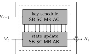
Mj Hj−1
Hj state update
SB SC MR AK key schedule SB SC MR AC
Fig. 2.An overview of the Whirlpool compression function. The 10-round block
cipherW with key schedule and state update is used in Miyaguchi-Preneel mode.
The functionality of the linear part of the primitive is to make sure that there are no narrow trails, i.e. trails where only a small number of S-boxes has a non-zero input difference. An S-box with a non-zero input difference is called
active. Let z denote a lower bound for the number of active S-boxes in a trail. Then it follows easily that (pS)z upper bounds the probability of a trail.
4.2 Whirlpool
Whirlpool is an iterative hash function based on the Merkle-Damg˚ard design principle [11,35]. It processes 512-bit message blocks and produces a 512-bit hash value. An unambiguous padding method is applied to ensure that the message length is a multiple of 512 bits [2]. Letm=M1kM2k · · · kMtbe at-block message (after padding). The hash valueh=H(m) is computed as follows (see Figure 2):
H0=IV,
Hj =W(Hj−1, Mj)⊕Hj−1⊕Mj, for 0< j≤t, h=Ht,
where IV is a predefined initial value and W is a 512 bit block cipher used in the Miyaguchi-Preneel mode [34].
4.3 The Block Cipher W
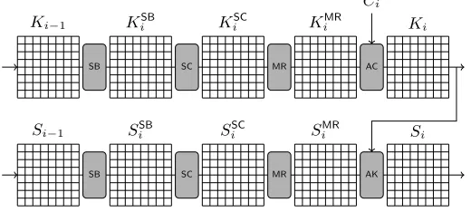
The block cipher W is designed according to the wide trail strategy and its structure is very similar to the Advanced Encryption Standard (AES) [36]. The state update transformation and the key schedule update an 8×8 state S, respectivelyK, of 64 bytes in 10 rounds. In one round, the round transformation updates the state by means of the sequence of transformations
AK◦MR◦SC◦SB, while the key schedule applies
Si−1 SSBi SiSC SiMR Si
SB SC MR AK
Ki−1 KiSB KiSC KiMR Ki
SB SC MR AC
Ci
Fig. 3. One round of the block cipher W, used in the Whirlpool compression
function.
to the round key. In the remainder of this paper, we will use the outline of Figure 3 for one round. We denote the resulting state after round iby Si and the intermediate states afterSubBytes (SB) bySSB
i , afterShiftColumns(SC) by SSC
i and afterMixRows (MR) by SiMR. The initial state prior to the first round is denoted by S0=Mj⊕Hj−1. The same notation is used for the key schedule with round keysKi withK0=Hj−1. Note that we changed the names of some steps of the round transformation of the original description [2] in order to be more similar to the AES nomenclature [10].
4.4 The Round Transformations of W
In the following, we briefly describe the round transformations of the block cipher W used in the Whirlpool compression function.
SubBytes (SB). TheSubBytesstep is the only non-linear transformation of the cipher. It is a permutation consisting of an S-box applied to each byte of the state. The 8-bit S-box is composed of 3 smaller 4-bit mini-boxes (the exponential E-box, its inverse, and the pseudo-randomly generated R-box). For a detailed description of the S-box we refer to [2].
ShiftColumns (SC). The ShiftColumns step is a byte transposition that cycli-cally shifts the columns of the state over different offsets. Column j is shifted downwards byj positions.
MixRows(MR). TheMixRowsstep is a permutation operating on the state row by row. To be more precise, it is a right-multiplication by an 8×8 matrix over F28. The coefficients of the matrix are determined in such a way that thebranch
Table 1.The number of differentials and possible pairs (a, b) for the Whirlpool S-box. The first row shows the number of impossible differentials and the last row corresponds to the zero differential.
solutions frequency
0 39655
2 20018
4 5043
6 740
8 79
256 1
AddRoundKey (AK) and AddRoundConstant (AC). The key addition in the state update transformation is denoted byAddRoundKeyand in the key schedule byAddRoundConstant, respectively. In this transformation the state is modified by combining it with a round key with a bitwisexoroperation. While the round key in the state update transformation is generated by the key schedule, it is a predefined constant in the key schedule.
4.5 Differential Properties of Round Transformations
In this section, we describe the differential properties of the round transforma-tions of Whirlpool.
SubBytes (SB). SubBytes has the following differential properties. Let a, b ∈ {0,1}8. Exhaustively counting over all 216 differentials shows that the number of solutions to the following equation
Si(x)⊕ Si(x⊕a) =b, (20)
can only be 0, 2, 4, 6, 8 and 256, which occur with frequency 39655, 20018, 5043, 740, 79 and 1, see Table 1. The task to return all solutionsxto (20) for a given differential (a, b) is best solved by setting up a precomputed table of size 256×256 which stores the solutions (if there are any) for each (a, b).
However, it is easy to see that for any permutationSi (to be more precise, for any injective map) the expected number of solutions to (20) is always one:
2−16X a
X
b
#{x| Si(x⊕a)⊕ Si(x) =b}= 2−16 X
a
28= 1,
because for a fixeda, every solutionxbelongs to a uniqueb. Since all the S-boxes are independent, the same reasoning is valid for the fullSubBytestransformation.
Table 2. Approximate probabilities (as base 2 logarithms) for the propagation of truncated differences through MixRows with predefined positions. a denotes the number of active bytes at the input andbthe number of active bytes at the output ofMixRows.
a\b 0 1 2 3 4 5 6 7 8
0 0 × × × × × × × ×
1 × × × × × × × × 0
2 × × × × × × × −8 −0.0017 3 × × × × × × −16 −8 −0.0017 4 × × × × × −24 −16 −8 −0.0017 5 × × × × −32 −24 −16 −8 −0.0017 6 × × × −40 −32 −24 −16 −8 −0.0017 7 × × −48 −40 −32 −24 −16 −8 −0.0017 8 × −56 −48 −40 −32 −24 −16 −8 −0.0017
row are moved to 8 different rows of the state. Hence,ShiftColumnsensures that the 8 bytes of one row of a state are processed independently in the subsequent
MixRowstransformation.
MixRows (MR). Since theMixRowsoperation is a linear transformation, stan-dard differences propagate throughMixRows in a deterministic way. The prop-agation only depends on the values of the differences and is independent of the actual value of the state. In case of truncated differences only the position, but not the value of the difference is determined. Therefore, the propagation of truncated differences through MixRowsis probabilistic.
Since the branch number ofMixRowsis 9, a truncated difference with exactly one active byte will propagate to a truncated difference with 8 active bytes with a probability of 1. On the other hand, a truncated difference with 8 active bytes can result in a truncated difference with 1 to 8 active bytes afterMixRows. The probability of an 8 to 1 transition is only 2−7·8 = 2−56, since we need 7 out of 8 truncated differences to be zero. In general, the probability of any a to b transition with 1≤a, b≤8 satisfyinga+b≥9 is approximately 2(b−8)·8. Note that the probability depends on the direction of the propagation of truncated differences, see Table 2.
AddRoundKey (AK) andAddRoundConstant (AC). SinceAddRoundKeyand
AddRoundConstant are simple xoroperations with a round key or a constant. Therefore, both standard differences and truncated differences propagate through
AddRoundKeyandAddRoundConstantin a deterministic way.
4.6 Good Differential Trails
S0 S1 S2 S3 S4 SB
SC MR AK
SB SC MR AK
SB SC MR AK
SB SC MR AK
Fig. 4. A 4-round differential trail with the minimum number (81) of active
S-boxes.
construct good differential trails by hand as shown in this section. We will use the following notation to specify the number of active bytes in two subsequent states in the state update:
a ri
−→b,
withathe number of active bytes in the first state,bthe number of active bytes in the second state andri thei-th round of Whirlpool. As an example, for one round ri of Whirlpool, we either get a+b ≥9 or a=b= 0, due to the design of theMixRowstransformation. Hence, for a= 1 we always get:
1 ri
−→8.
It follows from the properties of theShiftColumnsandMixRows transforma-tions, that any 4-round (truncated) differential trail has at least 92= 81 active S-boxes. Hence, (pS)z = (2−5)81 upper bounds the probability of any 4-round
differential trail (see Section 4.1). An example differential trail with 81 active S-boxes is given in Figure 4. Note that the active byte in stateS0 and stateS4 can be placed at any position (stateS1andS3change accordingly). The number of active S-boxes in each state for these trails are as follows:
1 r1
−→8 r2
−→64 r3
−→8 r4
−→1
This 4-round trail will be used to explain the principles of the rebound attack in Section 5.1. Note that this trail can be extended in a simple and straightforward way in the forward and in the backward direction. We will use the following trail to show a near-collision attack for the Whirlpool hash function in Section 5.4:
8 r1
−→1 r2
−→8 r3
−→64 r4
−→8 r5
−→1 r6
−→8
Another possibility is to extend the trail by adding rounds in the middle. If we add a second full active state in the middle, then we still get a valid trail. This trail will be used to extend the rebound attacks on the hash function by one round (see Section 5.3 and 5.4):
1 r1
−→8 r2
−→64 r3
−→64 r4
−→8 r5
−→1
Moreover, two full active states allow us to place one or two states with 8 active bytes in between them, such that all properties of the round transformations are still fulfilled:
1 r1
−→8 r2
−→64 r3
−→8 r4
−→8 r5
−→64 r6
−→8 r7
−→1
5
Attacks on the Hash Function
In this section, we describe the application of the rebound attack to reduced variants of the Whirlpool hash function. First, we describe the basic idea of the attack for Whirlpool reduced to 4.5 rounds. By improving the inbound phase of the attack, the complexity can be significantly reduced to about 264compression function evaluations and negligible memory requirements. Furthermore, we show how the attack can be extended to 5.5 rounds by adding another full active state in the inbound phase. The resulting attack has a complexity of about 2120 and memory requirements of 264.
Second, we present near-collision attacks for the Whirlpool hash function reduced to 6.5 and 7.5 rounds. These attacks are straight forward extensions of the collision attacks on 4.5 and 5.5 rounds, respectively. By adding 2 rounds in the outbound phase, we get a near-collision for the Whirlpool hash function reduced to 6.5 and 7.5 rounds.
5.1 Collision Attack on 4.5 Rounds
The rebound attack on 4.5 rounds of Whirlpool uses a differential trail with the minimum number of active S-boxes according to the wide trail design strategy. For this attack, the full active state is placed in the middle of the trail (see Figure 5):
1 r1
−→8 r2
−→64 r3
−→8 r4
−→1 r4.5
−−→1
To find a message pair following this 4.5-round differential trail, we first split the block cipherW into three sub-ciphersW =Wfw◦Win◦Wbw, such that the full active state of the differential trail is covered by the inbound phaseWin.
Wbw=SC◦SB◦AK◦MR◦SC◦SB
Win=MR◦SC◦SB◦AK◦MR
Wfw=SC◦SB◦AK◦MR◦SC◦SB◦AK
In the inbound phase, the actual values of the state are chosen to guarantee that the differential trail in Win holds. The differential trail in the outbound phase (Wfw, Wbw) is supposed to have a relatively high probability. While standard
xordifferences are used in the inbound phase, truncated differentials are used in the outbound phase of the attack. In the following, we describe the inbound and outbound phase of the attack in detail.
Inbound Phase. In the inbound phase of the attack we have to find inputs to
Winsuch that the differential trail inWinholds. It can be summarized as follows (see Figure 6).
S0 S1 S2 S3 S4 SSC4 SB
SC MR AK
SB SC
MR AK
SB SC MR
AK
SB SC MR AK
SB SC
outbound phase inbound phase outbound phase
Fig. 5.Differential trail for the collision attack on 4.5 rounds of Whirlpool. Black
state bytes are active.
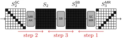
SSC
2 S2 S3SB SMR3
MR
AK SB
SC MR
step 1
step 2 step 3
Fig. 6. Inbound phase of the attack on 4.5 rounds of Whirlpool. Black state
bytes are active.
2. We choose a difference for the active byte in each row at the input ofMixRows
in roundr2(S2SC) and compute forward to the input ofSubBytesof roundr3 (S2). Note that this can be done for all 255 (∼28) values (nonzero difference) of the active byte for each row independently, which facilitates the attack. 3. In the next step of the inbound phase, thematch-in-the-middle step, we look
for a matching input/output difference of the SubBytes layer of round r3. This is done as described in Section 4.4 with a precomputed 256×256 S-box lookup table. As explained in Section 4.4, the expected number of solutions is one per trial. Note that we can search for S-box matches for each row of S2 and S3SB independently. Since we have 2
8 candidates for each row ofS 2 (and 1 for each row ofS3SB) the expected number of solutions for each row is 28(i.e. 2 solutions for each S-box). Hence, the expected number of solutions for the wholeSubByteslayer (8 rows) equals 264. In other words, we can find 264 actual values that follow the differential trail in the inbound phase with a complexity of about 28 round transformations.
Since we can repeat these 3 steps 264 times, we can find 2128actual values that follow the differential trail in the inbound phase.
Outbound Phase. In contrast to the inbound phase, we use truncated
the MixRows transformation, both in the backward and forward direction (see Figure 5). The propagation of truncated differentials through theMixRows trans-formation can be modeled in a probabilistic way, see Section 4.4. Since we need to fulfill one 8 to 1 transition in the backward and forward direction, the prob-ability of this part of the outbound phase is 2−2·56 = 2−112. Furthermore, to construct a collision at the output (after the feed-forward), we need that the differences at the input and output cancel out. Since only one byte is active, this has a probability of approximately 2−8. Hence, the probability of the outbound phase of the attack is 2−112·2−8= 2−120. In other words, we need to generate 2120starting points for the outbound phase to find one collision.
Since we can find one of these starting points in the inbound phase with an average complexity of 1, we can find a collision for the Whirlpool hash function reduced to 4.5 rounds with a complexity of about 2120 and negligible memory.
5.2 Improving the Collision Attack on 4.5 Rounds
In this section, we show how the complexity of the collision attack presented in the previous section can be improved significantly. The main idea is to extend the inbound phase of the attack by 1 round such that one 8 to 1 transition of the outbound phase is covered in the inbound phase of the attack. This improves the probability of the outbound phase significantly from 2−120to 2−56−8= 2−64. In other words, we need to construct only 264instead of 2120starting points for the outbound phase of the attack in the inbound phase. In the following, we show how to find inputs that follow the differential trail in the inbound phase of the attack with the following sequence of active bytes:
1 r1
−→8 r2
−→64 r3
−→8
Note that the attack is very similar to the attack on the hash function Grøstl in [29]. It can be summarized as follows.
1. Similar to the previous section, we first choose a difference for the 8 active bytes at the output ofMixRows of roundr3 (S3MR) and propagate backward to get the differences of the full active state at the output of SubBytes of roundr3(S3SB).
2. In the second step we choose a difference for the active byte in each row at the input ofMixRowsof round r2 (S2SC) and compute forward to the input ofSubBytes of round r3 (S2). Again, we can choose 28 differences for each row and compute each row independently.
3. Next, we look for a matching input/output difference of theSubBytes layer of roundr3 for each row ofS2 and S3SBindependently. This is done with a precomputed 256×256 lookup table as described in Section 4.4. Since the expected number of solutions per trial is one and we have 28 candidates for each row ofS2the expected number of solutions for each row equals 28, i.e. 2 solutions for each S-box.
4. For all 28 solution of each row of S
2, we compute backward to S1. Since
S0 S1 S2 S3 S4 S5 S5SC SB
SC MR AK
SB SC
MR AK
SB SC MR AK
SB SC MR
AK
SB SC MR AK
SB SC
outbound phase inbound phase outbound phase
Fig. 7.Differential trail for the collision attack on 5.5 rounds of Whirlpool.
andAddRoundKeyare byte-wise operations, this determines only 8 bytes of S1and the according differences (active bytes). In detail, we get 28candidates for each active byte in S1 after testing all 28 solutions for each row of S2 independently. Hence, we get 264 candidates for the 8 active bytes in row 1 of S1 after this step of the attack with a complexity of about 28 round transformations.
5. In order to follow the differential trail in the inbound phase of the attack, we have to guarantee that the differences inS1propagate from 8 to 1 active byte through theMixRows transformation in the backward direction. Therefore, we compute all 28differences of the single active byte at the input ofMixRows
in roundr1(S1SC) forward to the input ofSubBytesin roundr2(S1) and check for a match. Since we have 264candidates for the active bytes inS2, i.e. 28for each active byte, the expected number of solutions is 28 after testing all 28 candidates for the one active byte inSSC
1 . In other words we get 28solutions (actual values) that follow the differential trail in the inbound phase of the attack with a complexity of about 28 round transformations.
Since the probability of the outbound phase of the attack is 2−64, we need to repeat steps 1-5 about 256times to generate 264starting points for the outbound phase of the attack. Since we can find 28starting point for the outbound phase with a complexity of 28, we can construct a collision for the Whirlpool hash function reduced to 4.5 rounds with a complexity of about 264.
5.3 Collision Attack on 5.5 Rounds
In this section, we present a collision attack for the Whirlpool hash function reduced to 5.5 rounds with a complexity of about 2184−s and memory require-ments of 2s, with 0≤s≤64. The attack is a straightforward extension of the collision attack on 4.5 rounds of Whirlpool described in Section 5.1. By adding one round in the inbound phase of the attack we can extend the attack to 5.5 rounds (see Figure 7). This idea was introduced in [26], applied to the SHA-3 candidate Grøstl in [32], and called super-sbox cryptanalysis in [17]. In the 5.5 round collision attack, we use the following sequence of active bytes:
1 r1
−→8 r2
−→64 r3
−→64 r4
−→8 r5
−→1 r5.5
−−→1
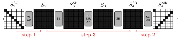
S2SC S2 S3SB S3 S4SB S4MR
MR
AK SB
SC MR AK
SB MRSC
step 1 step 3 step 2
Fig. 8.The inbound phase of the collision attack on 5.5 rounds of Whirlpool.
Win, while the trail in the outbound phase (Wfw, Wbw) can be fulfilled with a relatively high probability.
Wbw=SC◦SB◦AK◦MR◦SC◦SB
Win=MR◦SC◦SB◦AK◦MR◦SC◦SB◦AK◦MR
Wfw=SC◦SB◦AK◦MR◦SC◦SB◦AK
Since the outbound phase is identical to the attack on 4.5 rounds, we only discuss the inbound phase of the attack here (see Figure 8).
Since the outbound phase of the attack has a probability of 2−120, we have to generate 2120 starting points in the inbound phase of the attack. This can be summarized as follows.
1. Start at the input of MixRows in round r2 (SSC2 ) with arbitrary nonzero differences in the 8 byte positions indicated on Figure 8. Propagate the difference forward to the input ofSubBytesin roundr3(S2). Since we have one active byte in each row of the state this results in a full active stateS2. 2. Start with an arbitrary difference in the 8 active bytes at the output of
MixRowsin roundr4(S4MR) and compute backward to the output ofSubBytes in round r4 (S4SB). Again, since we start with one active byte in each row, we get a full active state inSSB
4 .
3. Next we have to connect the states S2 and SSB4 such that the differential trail holds. Note that this can be done for each row ofSSB
4 independently, which facilitates the attack. It can be summarized as follows.
(a) For all 264 actual values of the first row ofSSB
4 compute backward toS2 and check if the differential trail holds. SinceMixRowsworks on each row independently andShiftColumnsandSubBytes are byte-wise operations, this determines 8 bytes ofS2and the according differences. Hence, after testing all 264 candidates, the expected number of inputs such that the differential trail holds, is one.
(b) Do the same for row 2-8 ofSSB
4 .
After testing each row independently, the expected number of solutions is 1. Hence, we expect to get one actual value for stateSSB
To summarize, we can compute one starting point for the outbound phase of the attack with a complexity of about 264. Since we need 2120starting points in the inbound phase, the collision attack has a complexity of about 2184.
Note that the complexity of the inbound phase can be significantly reduced at the cost of higher memory requirements. By saving 2s candidates for the differences (active bytes) inS2, we can do a standard time/memory tradeoff with a complexity of about 2184−s and memory requirements of 2s with 0≤s≤64. Hence, by settings= 64 we can find a collision for the Whirlpool hash function reduced to 5.5 rounds with a complexity of about 2120and memory requirements of 264.
5.4 Near-Collision for Whirlpool
The collision attacks on 4.5 and 5.5 rounds can be further extended by adding one round at the beginning and one round at the end of the trail. The result is a near-collision attack on 6.5 and 7.5 rounds of the hash function Whirlpool. We use the following sequence of active bytes
8 r1
−→1 r2
−→8 r3
−→64 r4
−→8 r5
−→1 r6
−→8 r6.5
−−→8
for the near-collision attack on 6.5 rounds, and
8 r1
−→1 r2
−→8 r3
−→64 r4
−→64 r5
−→8 r6
−→1 r7
−→8 r7.5
−−→8
for the near-collision attack on 7.5 rounds. In the following, we summarize the attack for 7.5 rounds. Note that the attack on 6.5 rounds works similar. Since the inbound phase is identical to the collision attack on 5.5 rounds, we only discuss the outbound phase here.
First, note that the 1-byte difference at the beginning and end of the 5.5 round trail will always result in 8 active bytes after oneMixRowstransformation. Thus, we can go both backward and forward 1 round with no additional costs. After the feed-forward, the position of two active bytes match and cancel each other with a probability of 2−16. In other words, the outbound phase of attack has a probability of about 2−112 to construct a near-collision in 50 bytes and 2−128 to construct a near-collision in 52 bytes. Hence, we have to construct 2112 and 2128 starting points in the inbound phase of the attack to find a near-collision in 50 and 52 bytes, respectively. Since in the collision attack on 5.5 rounds one can construct 2s starting points in the inbound phase of the attack with a complexity of about 264 and memory requirements of 2s with 0 ≤s≤64 (see Section 5.3), the attack has a complexity of about 2176−sand 2192−s, respectively. Both attacks have memory requirements of 2s.
S0 S1 S2 S3 S4 S5 SB
SC
MR AK
SB SC MR AK
SB SC MR AK
SB SC MR AK
SB SC MR
AK
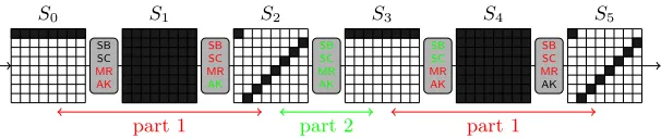
part 1 part 2 part 1
Fig. 11.The extended inbound phase of the attack on the compression function
of Whirlpool.
such that one 8 to 1 transition of the outbound phase is covered by the inbound phase of the attack (see Section 5.2). Hence, we can construct a near-collision in 50 and 52 bytes for the Whirlpool hash function reduced to 6.5 rounds with a complexity of about 256and 272, respectively.
6
Attacks on the Compression Function
In this section, we will present attacks on the Whirlpool compression function. Since in an attack on the compression function, the attacker has full control over the chaining variable input, this can be used to extend the previous attacks to more rounds. In detail, we can show a semi-free-start collision for the Whirlpool compression function reduced to 7.5 rounds and a semi-free-start near-collision for 9.5 rounds. The basic idea is to have an extended inbound phase consisting of two instead of one inbound phase and connect them by choosing the subkeys accordingly. The outbound phase of the attacks are identical to the previous attacks on the Whirlpool hash function on 5.5 and 7.5 rounds (see Section 5). In the following, we describe both, the extended inbound phase and the outbound phase of the attack in detail.
6.1 The Extended Inbound Phase
In this section, we describe the extended inbound phase consisting of 2 indepen-dent inbound phases in detail. We use the following sequence of active bytes for the attack:
8 r1
−→64 r2
−→8 r3
−→8 r4
−→64 r5
−→8
In order to find inputs following the differential trail, we split the attack into two parts. In the first part, we have two inbound phases: one in round 1-2 and one in 4-5, with active bytes 8→64→8 each. In the second part, we need to find values for the subkeys such that the resulting differences in the 8 active bytes and the 64 (byte) values of the state between round 2 and 4 can be connected.
Part 1 (The 2 Independent Inbound Phases). This part of the attack
1. Inbound Phase 1 (round 1-2):
(a) Start with 8 active bytes at the output ofAddRoundKeyin roundr2(S2) and propagate backward to the output ofSubBytesin roundr2 (S2SB). (b) Start with 8 active bytes (1 in each row) at the input of MixRows in
roundr1(S1SC) and propagate forward to the input ofSubBytesin round r2(S1). Again, this can be done for all 28differences (value of the active byte) and for each row independently.
(c) Next, we look for a matching input/output difference of the SubBytes
layer of roundr2for each row ofS1 andSSB2 independently. This can be implemented with a precomputed 256×256 lookup table as described in Section 4.4. Since, on average, we get one solution per trial and we have 28 candidates for each row ofS
1, the expected number of solutions for each row is 28, i.e. 2 solutions for each S-box. After finishing this step we have 264 inputs (2 for each S-box ofS
1) that follow the differential trail in round 1-2.
2. Inbound Phase 2 (round 4-5): Do the same as in step 1 for rounds 4-5.
Note that after this part of the attack, we get 264 candidates for SSB
2 and 264 candidates forS4 with a complexity of about 29round transformations.
Part 2 (Connecting the 2 Inbound Phases). In the second part of the
attack, we have to connect the results of the two inbound phases. In detail, we have to ensure that the differences in the 8 active bytes (a 64-bit condition) as well as the actual values ofSSB
2 andS4(a 512-bit condition) match by choosing the subkeys K2, K3 and K4 accordingly. In other words, we have to solve the following equation:
MR(SC(SB(MR(SC(SB(MR(SC(S2SB))⊕K2)))⊕K3)))⊕K4=S4 (21) with
K3=MR(SC(SB(K2)))⊕C3 K4=MR(SC(SB(K3)))⊕C4.
(22)
Since we have 264candidates forSSB
2 , 264candidates forS4and can choose from 2512values for the subkeys (K
2,K3orK4because of (22)), the expected number of solutions is 264.
SinceSMR
2 =MR(SC(SSB2 )), we can rewrite (21) as follows:
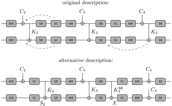
MR(SC(SB(MR(SC(SB(S2MR⊕K2)))⊕K3)))⊕K4=S4 (23) Note that in the Whirlpool block cipher the order ofShiftColumnsandSubBytes
can always be changed without affecting the output of one round. In order to make the subsequent description of the attack easier, we do this here and get the following equation:
MR MR
SB SB
SC SC
MR MR
SB SB
SC SC
MR MR
SB SB
C2
K2
C3
K3
C4
K4
original description:
MR MR
SC SC
˜ S2
SB SB
MR MR
SB SB
SC SC
X
MR MR
SB SB
C2
˜ K2
C3
K3
C4
C4
KSB
4
alternative description:
Fig. 12.The sequence of operations is changed to get an equivalent description
of theW.
˜
S2 S2 S3MR S3 S4SB X
AK MRSB AK SB AK
˜
K2 K3 K4SB
Fig. 13. The second part of the extended inbound phase of the attack on the
compression function of Whirlpool by using the alternative description.
Furthermore, MixRows and ShiftColumns are linear transformations and hence we can rewrite the above equation as follows:
SB(MR(SB( ˜S2⊕K˜2))⊕K3)⊕K4SB=X (25)
with ˜S2=SC(S2MR), ˜K2=SC(K2),K4SB=SB(K3),X =SC−1(MR−1(S4⊕C4)). Figure 12 shows how the sequence of operations between stateSMR2 and S4 of the Whirlpool state update and key schedule are changed. In the following, this equivalent description is used to connect the values and differences of the two states ˜S2 andX.
Remember that the differences of SSB
2 and S4 have already been fixed in part 1 of the attack. SinceShiftColumns,MixRows andAddRoundKeyare linear transformations, also the differences of ˜S2 and X are fixed. However, we can still choose from 264 candidates for each of the states ˜S
2andX, since we found 264 candidates forSSB
S4) row-by-row and independently. Hence, both the complexity and memory requirements for this step are 28 instead of 264.
Now, we use (25) to determine the subkey ˜K2 such that we get a solution for the extended inbound phase and hence, a starting point for the outbound phase of the attack. Note that we can solve (25) for each row of the states independently. It can be summarized as follows. (see Figure 13).
1. Since AddRoundKey is a linear transformation, we can compute the 8-byte difference inS2 (form ˜S2) and S4SB(from X). We want to stress that these differences are the same for all 264 candidates of the state ˜S
2 and all 264 candidates of the stateX, respectively.
2. Choose arbitrary values for the first row ofS2and compute forward to obtain the differences and values of the first row ofS3MR. Again, sinceAddRoundKey is a linear transformation, this also determines the difference ofS3.
3. Next, we choose the first row of the keyK3 such that the differential of the S-box betweenS3andS4SBholds. This can be done similar as in the inbound phase with a precomputed 256×256 lookup table as described in Section 4.4. 4. Once the first row of K3 is fixed we can also compute the first row of ˜K2
and KSB
4 . This also determines the first row (64 bits) of ˜S2 and the first row (64 bits) of X. Remember that we have 264 candidates for state ˜S
2 and 264 candidates for state X due to step 1. Hence, the expected number of compatible candidates for both ˜S2 and X equals 1. In other words, we can connect the values and differences of the first row of ˜S2 andX with an average complexity of one.
5. Next, we have to connect the values of ˜S2 and X for rows 2-8. Note that this can be done independently for each row by a simple brute-force search over all 264values of the corresponding row of ˜K
2. Since we have to connect 64 bits and we test 264 values for each row of ˜K
2 the expected number of solutions is one.
Since we can repeat the above procedure 264 times with different values for the first row of S2, we get in total 264 solutions (matches) connecting state ˜S2 to state X with a complexity of 2128 and memory requirements of 28. In other words, we get 264 starting points for the outbound phase of the attack. Hence, the average complexity to find one starting point for the outbound phase is 264. Note that Step 5 can be implemented using a precomputed lookup table of size 2128. In this lookup table each row of the keyK2 (64 bits) is saved for the corresponding two rows of ˜S2 andX (64 bits each). Using this lookup table, we can find one starting point for the outbound phase with an average complexity of 1. However, the complexity to generate this lookup table is 2128. It is important to note that one can construct a total of 2192 starting points in the extended inbound phase to be used in the outbound phase of the attack.
6.2 Outbound Phase
through the adjacentSubByteslayers, we get a truncated differential in 8 active bytes in each direction. These truncated differentials need to follow a specific active byte pattern to result in a semi-free-start collision for 7.5 rounds and a semi-free-start near-collision for 9.5 rounds, respectively. In the following, we describe the outbound phase of the two attacks in detail.
Semi-Free-Start Collision for 7.5 Rounds. By adding 1 round in the
begin-ning and 1.5 rounds at the end of the trail, we get a semi-free-start collision for 7.5 rounds for the compression function of Whirlpool with the following sequence of active bytes:
1 r1
−→8 r2
−→64 r3
−→8 r4
−→8 r5
−→64 r6
−→8 r7
−→1 r7.5
−−→1
For the differential trail to hold, we require that the truncated differentials in the outbound phase first propagate from 8 to 1 active byte through theMixRows
transformation, both in the backward and forward direction (see Figure 14). Since the transition from 8 active bytes to 1 active byte through the MixRows
transformation has a probability of about 2−56, and the exact value of the input and output difference in one byte has to match after the feed-forward to get a semi-free-start collision, the outbound phase has a probability of 2−2·56−8 = 2−120. In other words, we have to generate 2120starting points (for the outbound phase) in the extended inbound phase of the attack.
Since we can find one starting point with an average complexity of about 264 and memory requirements of 28, we can find a semi-free-start collision with a complexity of about 2120+64= 2184. The complexity of the attack can be reduced to 2120by using a precomputed lookup table of size 2128in the extended inbound phase of the attack.
Semi-Free-Start Near-Collision for 9.5 Rounds. As in the attack on the
Whirlpool hash function, the semi-free-start collision attack on 7.5 rounds can be further extended by adding one round at the beginning and one round at the end of the trail in the outbound phase. The result is a semi-free-start near-collision for 9.5 rounds of the compression function with the following sequence of active bytes (see Figure 15):
8 r1
−→1 r2
−→8 r3
−→64 r4
−→8 r5
−→8 r6
−→64 r7
−→8 r8
−→1 r9
−→8 r9.5
−−→8
7
Distinguisher for the Whirlpool Compression Function
Now we will show how the compression function attack described in Section 6 can be used to show a certificational weakness in the full Whirlpool compression function. To be more precise, we will show how to distinguish the Whirlpool com-pression function from a random (that is, randomly selected) one-way function using the results described in Section 3.
Obviously, the difference between two Whirlpool states can be seen as a vector in the vector space of dimension N = 512 over F2. The crucial observation is that the attack of Section 6 can be interpreted as an algorithm that can findt difference vectors in F512
2 (output differences of the compression function) that form a subspace Vout ⊆ F5122 with dim(Vout) ≤128. To see this, observe that by extending the differential trail from 9.5 to 10 rounds, the 8 active bytes in SSC
10 will always result in a full active state S10 due to the properties of the
MixRows transformation. Thus the near-collision is destroyed. However, even though after the application ofMixRowsandAddRoundKey the stateS10is fully active in terms of truncated differences, thexordifferences inS10still belong to a subspace ofF5122 of dimension at most 64 due to the properties ofMixRows. If we look again at Figure 15, both the differences inS0 (respectively the message blockMj) and the differences inSSC10 can be seen as (difference) vectors belonging to subspaces ofF5122 of dimension at most 64. Therefore, after the feed-forward, we can conclude that the differences at the output of the compression function form a subspaceVout⊆F5122 with dim(Vout)≤128
Hence, we can use the attack of Section 6 to find t input differences such that the corresponding output differences form a vector spaceVout of dimension n≤128. This has a complexity oft·2176ort·2112 using a precomputation step with complexity 2128. Note that t ≤ 2192−112 = 280, due to the restrictions in the extended inbound phase of the attack (see Section 6.1).
Now the main question is for which values oft our attack is more efficient than the generic attack. In other words, how do we have to choosetsuch that we can distinguish the compression function of Whirlpool from a random one-way function. Table 3 compares for several values oftthe complexity of our dedicated approach to the query complexity in the generic case (cf. Section 3).
As can be seen in the table, the Subspace Problem for the full Whirlpool compression function is easier to solve than for a random one-way function when we taket= 212. The complexity of the attack is then about 2188. The probability to solve the Subspace Problem when makingQ= 2188queries to a random one-way function with the parameterst = 212, N = 512 and n= 128 is ≈2−30833. This follows from Proposition 1. Therefore, we get a distinguishing attack on the full Whirlpool compression function. Note, that by using a precomputation table as described in Section 6, the complexity reduces to 2121 witht= 29.