Centre for Advanced Spatial Analysis University College London
1-19 Torrington Place Gower Street
London WC1E 6BT
Tel: +44 (0) 20 7679 1782 Fax: +44 (0) 20 7813 2843 Email: [email protected] http://www.casa.ucl.ac.uk
http://www.casa.ucl.ac.uk/angularanalysis.pdf
Date: April 2000
ISSN: 1467-1298
Introduction
This paper presents a method for the quantification of a spatial layout for the purposes of prediction of movement through or occupancy of the space. We call this method the 'angular analysis' of the space.
The method itself is straightforward and simply embodies the combination of two ideas. Firstly, the prediction that if a body, e.g., a person or means of transportation such as a car or a ship, is to travel from point A to point B, then it will attempt to turn as little as possible (rather than the more usual assumption that it will try to follow the shortest path between A and B). Secondly, that any point in the considered space can be a start or an end point to a journey, and any journey from any start to any end point is equally likely as any other journey. The combination of these two ideas is used as a basis for quantification of points within the space.
This paper shows how these ideas are linked intrinsically with the notion of ‘space syntax' as proposed by Hillier and Hanson 1984 and later Hillier 1996, and other methods currently used for similar purposes. We give formal definitions of angular analysis methods and demonstration algorithms for the calculation.
The structure of the paper is as follows. In section 2, we very briefly outline the context of the angular analysis method within methods of prediction and simulation of movement and occupancy. Section 3 introduces the key concepts of angular analysis, while section 4 considers its position relative to other methods, looking in more detail at how it relates to space syntax, gravity modelling and autonomous agents. Section 5 discusses the mathematical detail for the metrics that will constitute angular analysis, and section 6 looks at methods for implementing the analysis. Finally, some concluding remarks are given in section 7.
Context
correspondence with gravity modelling (although a reworking of the concepts of gravity models is required), and also that the method can be applied to a simulation using autonomous agents.
Angular analysis can be seen as overlapping many areas, although it is most allied to space syntax. At present the primary use envisaged for the method is the prediction of people and traffic movement in building and urban environments. Space syntax is a successful predictor for people movement patterns at this level. Where angular analysis hopes to improve is to give a finer level of detail to the method and open up possibilities in the three-dimensional analysis of space. In addition, a more accurate representation of where movement actually occurs should be achievable.
In addition, angular analysis also hopes to build bridges to other forms of urban modelling. An important feature of angular analysis is the ability to build in factors such as trip length, model weighting using measured vehicle flows and details such as one-way streets, although the approach of angular analysis is still concerned with a method of quantification through the layout of the space itself and not through the basis of a psychological perception or an empirical model.
Finally, it should be noted that most areas of traffic modelling, for example, kinematic wave theories (such as the LWR model of traffic flows, Lighthill & Whitham, 1955, Richards, 1956), have little in common with the angular analysis method, and the working described here can only be applied over the top of these schemes after finishing the angular analysis to provide, for example, more realistic driver choices at route intersections.
Key concepts for angular analysis
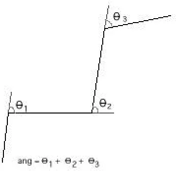
Figure 0-1 Path angle calculation
We must be clear that when we talk about the change in direction along a path, we are talking about the absolute change of direction as a body moves from point A to B. Figure 3-1 shows how the angle turned through on the journey is calculated. Note that the angles that are added are always positive — this is necessary to form sensible interpretation of angular change along a path.
1.1 Directed search: Minimum Angular Path
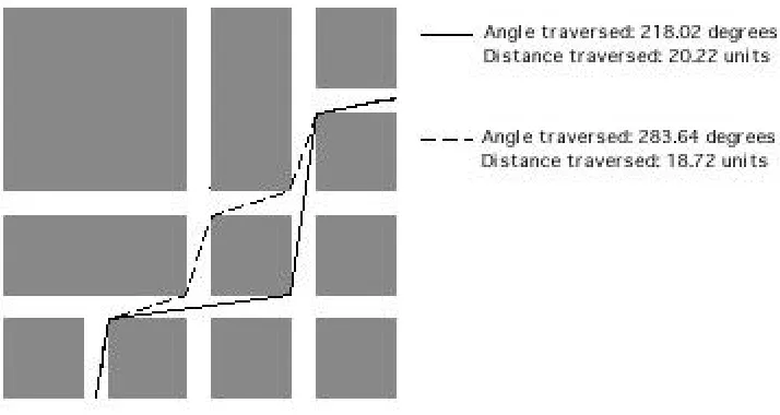
The key concept for angular analysis is the idea that a body will turn as little as possible to achieve a route from A to B. That is, the body will choose the route which will result in the minimum change in direction. We call the route with the minimum change in direction the minimum angular path between A and B, (or MAP for short). This is in contrast to the minimum distance path (or minimum Euclidean path) between the two points.
Figure 0-2 The minimum Euclidean path and the minimum angular path between two points on simple 2D spatial
layout
Whether or not real bodies choose this route is not an issue to the angular analysis of a space, which is merely concerned with the quantification of a space in terms of its layout. Indeed, it is certain that there are more complex issues at work in the movement of people, cars, ships and so on, and if the method is to provide useful information, it will have to be combined with other methods of movement prediction. As a facile example, it might be observed that a tourist in London will travel from Tottenham Court Road station to Picadilly Circus travelling down Charing Cross road and across Shaftsbury Avenue, while a local will travel through the centre of Soho to achieve the same goal. In doing so, the tourist has chosen to follow the minimum angular path, whereas the local has chosen the minimum Euclidean path. In this case, any complete movement prediction would have to predict both the movement of the tourist (which the minimum angular path does) and the movement of the local. The complete prediction system might weight the number of locals to tourists, the numbers arriving at each tube station, those by car, and so on and so on. Angular analysis does not claim to be that prediction system, but merely a quantification of space useful to the prediction of movement or occupancy.
1.2 Undirected search: Angular Separation
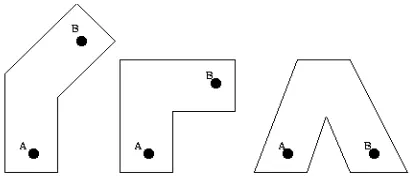
Figure 3-3 shows three systems, each system progressively requiring more angular turn to get from point A to B. We might say that a body starting at A is less likely to reach the destination B in each case from left to right (or at least, find it more difficult to locate B in each case), as the angular separation increases.
If a body always follows the minimum angular path by preference, then the likelihood of reaching any point is strictly proportional to the angular separation of the points. If a body chooses to follow all the zero angle paths, followed by all the one degree paths, and so on, then it will only find locations by following the minimum angular path to all locations.
Of course, an independent body will not have full knowledge of the system, and therefore, while performing undirected search, may well follow the path of expected minimum angle, rather than actual minimum angle. The formulation of an expected minimum angular path is discussed further in section 4.3.
1.3 Quantification of space through the minimum angular path
So far we have only looked at single paths, and single outcomes of a journey from A to another point in the system, B. We now make the assumption that any point in the system is a valid starting point and any point a valid endpoint to a path.
We investigate two types of analysis, with the working titles 'movement' and 'occupancy'. The quantities are not meant to be literally movement and occupancy, but as descriptions they look as though they might have some intuitive similarity.
The 'movement' method quantifies the numbers of bodies moving along the paths in the system, whereas the 'occupancy' method quantifies the likelihood of a body arriving at a point within the system. We should note at this point that if the quantities were to be taken literally, the two
measures would be co-dependent: the amount of movement to a location depends on the likelihood of going there, and the occupancy depends on the amount of movement to (and through) that space.
For movement, we look at the paths bodies take between all pairs of points in the system (as if all points were equally likely starting points and destinations), as shown in figure 3-4. We then sum these paths at all points within the space to quantify the movement potential at any point within the system. Accordingly, our ‘movement' metric is the minimum angular path summation, or for short, the MAP summation of the space.
Figure 0-4 Calculating the 'movement' metric
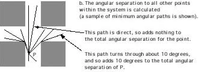
For occupancy, we look at the location, and the likelihood of reaching that location from all points in the space. One caveat: we have said that the likelihood of reaching the location depends on some function of the minimum angular path, but we have not specified what that is. For the time being, we will either sum or take the mean of the angular separation to all other points in the spatial system from this location, and assign a quantity for this location, as shown in figure 3-5. Our ‘occupancy' metric is therefore either the total angular separation or the mean angular separation of the point.
As already mentioned, these two metrics ignore the co-dependence of the quantities. For the time being we will ignore this co-dependence, but return to it later. For now, note that the two quantities are both based on the minimum angular path between points in the system, but one is concerned with the points joined in the system, while the other involves the paths between those points. Accordingly, it is some combination of the two types of representation that will give a 'unified' metric.
1.4 Summary
This section has introduced the key concepts in angular analysis. These are: the minimum angular path, the angular separation (along the minimum angular path), and the summation of these quantities: the MAP summation for the space and the total angular separation of a point. The actual metrics proposed, and more formal definitions are left to section 5.0. For now, we return to the context of angular analysis within current technology. As a final note to this section, although the discussion has been rooted in 2D examples, there is no reason why the concepts cannot be extended to 3D.
Comparisons with existing technology
As has already been mentioned, angular analysis has little to do with many of techniques used in pedestrian and traffic flow prediction and simulation. Many other techniques tend to concentrate on the necessary journeys needed connect A to B in economic terms, and do not tend to the epistemology of movement between locations. The reader might like to consider how long he or she has sat in a traffic jam contemplating whether or not to turn off along an empty side road, but not doing it. While a fluid dynamics representation may look at this in terms of flow and regard junctions as valves, and make predictions made from observed junction types, angular analysis (and also space syntax) is concerned with how the junction is related to the whole spatial system, and will make predictions on whether the driver will turn based on this alone.
1.5 Space Syntax
Space syntax is a general term for a group of techniques concerned with the representation and analysis of spatial layouts, first proposed by Hillier and Hanson, 1984. The key points are that some spatial representation is first chosen (these fit into categories such as convex spaces and axial lines — to be explained further) and then the configuration of this spatial representation is investigated. Put into these terms angular analysis is another one of these techniques: the spatial representation is of angular relationships within the space. The configurational analysis portion of the angular analysis method might be the summation that we talked of in section 3.3. However, as we shall see, angular analysis does not actually fit as succinctly as this into the space syntax paradigm, as the layers which form 'representational' and 'configurational' are not clearly defined in angular analysis.
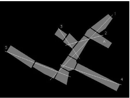
One key technique within space syntax is the 'axial analysis' of a space. It involves drawing a set of lines across the system (for example, a street network or building layout) and then weighting the lines according to their configuration. The result of this analysis is a map of lines coloured by weighting covering the system, which can be used for the prediction of people or traffic movement within that system.
The set of axial lines is the set of the fewest and longest lines of visibility and access that intersect. The set is chosen such that it covers every space within the system, where space is defined as a 'convex space' or the largest convex polygon of intervisible space. Figure 4-1 shows an example of a system broken into convex spaces, and then the axial lines drawn on this set of convex spaces.
Having drawn axial lines, a configurational analysis is performed. For example, the lines in the figure can be formed into a graph, connections being made where they intersect. In the figure, line 2 is connected to lines 1 and 3. We can find the global relationship of this line to others by questions such as what is the mean depth of the graph as viewed from line 2. Where a depth is the number of lines needed to cross from the start line. So lines 1 and 3 are one line away, or at a depth of 1 relative to line 2. Lines 4 and 5 have a depth of 2 relative to line 2, so the mean depth is (1 + 1 + 2 + 2) / 4 = 1.5. The mean depth of a line (with a few minor enhancements) gives a surprisingly good correlation with real people movement along the lines.
unnatural weighting to highly spatially complex areas of the space (where large numbers of axial lines are required).
Notice that axial analysis implicitly includes the notion of a number of turns needed to move from one space to another. By looking at the properties of a line of sight, we make a statement about the relationship of movement from one space to another within the system. If we are standing on an axial line (or within the space through which the axial line passes), the mean depth tells us the average number of turns it would need us to take to reach every other space within the system.
Figure 0-1 Convex and axial break-up of a spatial layout
However, isovist integration analysis can be seen as a special case of mean angular separation: if, rather than taking the precise angle in angular analysis, we take the case of 'no angular change = 0' and 'any angular change = 1', then we have defined isovist integration, as we have reduced the angular change to simply turning. Angular analysis is therefore a more finely tuned version of isovist integration.
However, angular analysis also incorporates the concept of MAP summation. The MAP summation does have a corresponding concept in isovist analysis: the sum of all paths with the minimum number of turns. But there is a problem here: there are not only a huge number of paths with the minimum number of turns, but from the angular analysis position, many 'ridiculous' paths. For example, if one 10 degree turn is need to get from A to B, then a turn of 170 degrees could also be a feasible path.
Finally with regard to space syntax, notice that the concept of a graph has been lost, and falls part way between the angular separation calculation and the angular separation totaling found in angular analysis. This is what was meant by saying that the configurational step has been blurred in angular analysis if it is treated solely as a space syntax technique.
1.6 Gravity Models
Gravity models for spatial systems are extremely sophisticated (see, for example, Erlander and Stewart, 1990). The drive behind most gravity models, however, remains objective driven (i.e., attraction is formulated according to the trips occurring from A to B), rather than spatially driven (if A happens to be going to B, then it will follow this path). Hence, a lot of gravity modelling is concerned with locating the trip densities rather than the routes taken for these trips. However, the scheme of attraction can be formulated to accommodate the angular model.
Attraction can be given by, for example:
Fi = ∑mi mj / dij2
bodies i and j rather than their Euclidean separation (debate about the distance function in gravity modelling is not new, although using the angular separation of locations is unknown).
The revised distance function can be then incorporated into the gravity model, where the mass units represent the trip densities at locations i and j. This discussion is obviously open to further research, but for the moment, we have shown that there is an application in the area of the distance metric used in gravity modelling.
1.7 Agent-Based Simulations
So far, little work has been done on navigation at the level of general movement with agent based simulations (as opposed to localisation through map construction), although there is emergent work in the field of robotics. Angular analysis can be used to add realism into the exploratory movement, or movement back home, of agents. Currently, this tends to concern simple methods, such as random search, while maintaining a direction vector to return home (this particular method is known as path integration, where much research has concerned the movement of ants).
We can add a component to the autonomous agent's psychology to tell it to follow the minimum angular path to return home, and during general search, to look for interesting locations. For the purposes of angular analysis, an interesting location is one that has low angular separation from the rest of the space. For the return journey, we may have constructed a map, making minimum angle path calculations easy, however, when performing undirected search, an agent has no idea about the global aspects of the space, so we must program for individual decision points at the local level. In angular analysis we must adapt the angular separation criterion to use an expected angular separation for the path. In the agent psychology we have a number of cases: for example, crossing an open space is relatively simple: the way to minimise angular separation is to continue in a straight line. However, when confronted with a choice, such as a continuing path forwards and one to the side, a decision must be based on the benefit of turning. Questions such as: 'how far can I continue in this current direction?' and 'would I be more sensible to turn now and keep going with turning less in the new direction?' must be asked.
turn on the new journey. For the part of the journey that is unseen in each case, the agent can base the angular turn needed on its own (continually updated) experience of how much it needs to turn within the system.
For example, if the agent can see 50m ahead and 60m at 10°, and so far it has traveled 350m and turned 70°. The anticipated turn for an unseen part of the journey is thus 70° / 350m = 0.2 degrees per metre. So by turning, the expected angular change is 10° (turn required) + 90° (after 60m) = 100°. By continuing, the expected angular change is 90° (after 50m) + 0.2° per metre for 10m = 110°. So in this case the agent would turn by 10° to maintain the lowest expected angular change.
As in the previous section, this discussion leaves open further research in this area. Here we have shown that angular analysis principles can be applied in the field of agent based simulations.
The definition of angular analysis
Up until now, we have focussed on a general discussion of principles. In this section, we give formal definitions for several angular analysis concepts, followed by a discussion of how to apply these concepts to an actual space, and finally we provide further discussion of more in-depth issues.
1.8 Concept Definitions
1.8.1 Minimum angular path
The minimum angular path (MAP) between two points, A and B, in a spatial system, comprised of open (accessible) space and closed (inaccessible) space is the route from A to B through open space with the minimum absolute angular change in direction. There may be more than one minimum angular path between two points. We refer to the kth MAP between points i and j in the system as pijk.
1.8.2 Angular separation
The angular separation between two points A and B, is the least change in absolute angle required to traverse from A to B through open (accessible) space. We refer to the (unique) angular separation of i and j as A(pij) (the angle traversed taking any minimum angular path between the
points).
The minimum angular path summation of the system or MAP summation of the system is the integral of the set of all minimum angular paths in the system. The set of all minimum angular paths is constructed by taking the set of all possible pairs of points in the open space of the system and connecting them with the set of k minimum angular paths between them. Where more than one MAP exists between a pair of points, that path is divided by the total number of possible MAPs between that pair of points.
That is:
µx = Σi Σj Σk pijk ^ x / Σk
Where µx is the MAP summation at point x within the system, Σi and Σj the sum over all points in
the system, subscripted i and j, pijk the set of k MAP(s) joining points i and j.
1.8.4 Total angular separation
The total angular separation of a point is the sum of the angular separation for all minimum angular paths to all other points in open space within the system.
That is:
Ti = ΣjA(pij)
Where Ti is the total angular separation of the point i, Σj the sum over all points j in the system, and
A(pij) the angular separation for the minimum angular path pij.
1.8.5 Applying angular analysis to a space defined in Euclidean coordinates
We now discuss the process for applying angular analysis to a real spatial system defined in terms of Euclidean coordinates. The closed space is marked as closed within polygonal or polyhedral regions throughout the otherwise assumed open space in a system, or vice versa.
suggested that an approximation to continuous space such as pixelisation (or quantisation) of the space is used. This is a standard technique used within computer science.
In addition, but possibly separately, the quantisation of angular values is needed. If it is assumed that a set of vectors comprises a path, then either the polar or Euclidean values of the vectors must be quantised. That is, there must be a set of discrete directions, rather than a set of continuous directions.
Figure 5-1 shows an example of pixelisation of a space combined with quantised vectors through the space and the resulting pixels that are counted as being on the MAP formed from these vectors.
Figure 0-1 The effect of pixelisation of a space
Once the space has been split in this way, MAPs may be calculated in many ways: a sample algorithmic solution is given in section 6.0, where the MAPs are computed in parallel. An alternative process for generating MAPs might more simply involve moving to each pixel, calculate all the zero angle paths to all other pixels, then all the x degree paths, then 2x degree paths and so on, until all the MAPs to all other pixels in the system are discovered. Whatever, the result is a set of MAPs in terms of vectors (direction and lengths) or pixel lists (a set of physically linked pixels).
The process thus renders values for the minimum angular path summation and mean angular separation for each pixel or other type of quantised unit. The process can be summarised as follows:
1.9 Discussion of problems and enhancements
A number of issues related to physical systems arise. This section is intended to outline a few of these, with brief descriptions of how the method can be enhanced to accommodate the features.
The mathematical and algorithmic solutions are left to further work.
1.9.1 Relative openness of space
The minimum angular path only takes account of open and closed space, and no in between. In an actual system, there will be areas of relative openness, for example, for a pedestrian, a busy road is less open than a pavement, and a crossing is only open to either pedestrians or traffic for a percentage of total time. This can be incorporated into angular analysis by varying the values of paths through the semi-open space, by means of a permeability value. A minimum path would be 'scored down' by some percentage openness value, thus giving priority to a perhaps more deviating path. An ideal model would incorporate both deviating paths and the true minimum path according to their relative percentage scores.
1.9.2 Varying trip lengths
Quantise the entire spatial system
Discover the set of minimum angular paths for every pair of quantised units
For every quantised unit, count the number of MAPs crossing unit
For every MAP, calculate the absolute angular change
Attribute this value to the quantised unit at the start of the MAP.
Sum this value to give the MAP summation for each quantised
The Euclidean length of the minimum angular path has not yet been taken into account. This is perhaps the easiest to incorporate, and useful since it significantly decreases the processing time. Several examples are: in the case of a human body, the average or maximum trip length (for example, 1km) might be used to cut off the minimum angular path calculation at a certain distance from the starting point. In the case of a car journey, this could be increased to, for example, 5km. This saves processing time, and gives more realistic movement prediction.
1.9.3 One-way streets
For traffic flows, the presence of one way streets can be dealt with by allowing only paths that follow the general direction of the street. For example, the group of pixels that form a street (or segment) can be marked by hand as going 'East'. 'East' might only allow vectors with a direction in the range 45° to 135° to pass through these pixels.
1.9.4 Calibration through boundary conditions
Boundary conditions can be used at the system edges to fix the number of bodies entering and exiting the system (according to observed flows). The minimum angular paths can be calibrated by allocating weights to the minimum angular paths from the edges of the system. Rather than assigning a value of '1' to each pixel that is crossed, a value according to the number of bodies entering through that point. Then, only the MAPs from these points are calculated. Further extensions include: to move to the endpoints of the MAPs from the edges and then to calculate the MAPs from these points, using some reducing function of the flow to that point; to use the entrance and exit flows, so that the entrance and exit to the system is equated, then calculate the scaling of all MAPs accordingly.
1.9.5 Iterative combination of 'movement' and 'occupancy' metrics
in the system). This process is continued until the amount of 'particle' arriving at any point is in equilibrium (i.e., the amount of 'particle' arriving is the same as it was the last time all the calculation was performed). Whether any system does actually reach equilibrium through this method has not been tested yet.
1.9.6 Global system quantification
In addition to the local quantities of MAP summation at each point and the total angular separation of each point, combination of the quantities is possible to give some sort of calibration of, for example, how 'hard' a certain system is to navigate. A mean and standard deviation of the MAP summation will show how much of the system is 'used' through angular interaction. A mean of the mean angular separation might give a value for how 'difficult' the system is to comprehend.
Proposed algorithms
This section identifies an algorithmic solution to the calculation of angular analysis quantities. This is not the only algorithmic solution to the problem: its presence here is only to show that angular analysis may be implemented through a computer program.
Pixel number 1 2 3 4
1 0° no value yet no value yet 40°
(3 c,e 4 j,x 1)
10° (4 j,x 1)
2 0° 20°
(3 c,k 2)
60° 50° (4 e,c 3 c,k 2)
3 0° 30°
(4 e,c 3)
4 0°
In this example, a pair of vectors 'c' and 'e' is discovered that joins pixels 3 and 4 with an angle of 30°. The knock-on effect of this is to assign a value of 40° to the not yet discovered relationship between pixels 1 and 3, because pixel 3 is joined to 4 by 30° and pixel 4 is joined to pixel 1 by 10°. Similarly, the angle between pixel 4 and pixel 2 is updated 50° from a previously calculated figure of 60°. At the same time, the new minimum angular paths can be written, for example, the path from pixel 4 to 3 is inserted: pixel 4, via vector 'e' then vector 'c' to pixel 3. Similarly, the revised path for pixel 4 to pixel 2 is: pixel 4 to pixel 3 (via vectors e and c), then pixel 3 to pixel 2 (via vectors c and k).
Figure 0-2 Two vectors at angle θ cross, the pixels along the vector are attributed with the angle of incidence
At the end of joining all vectors to all other vectors, the pixel matrix is left with all minimum angular paths between pixels and all angular separations between pixels. This can then be used to calculate the minimum angular path summation for the system, and the total angular separation for any pair of pixels, with ease. The angular separation for every pair of points is already present, so summing a row from the matrix gives the total angular separation. The minimum angular path must be worked out from each path by using the vector crossing point (note that in Euclidean geometry, each pair of vectors can only cross once). A table of vector crossing points is easy to construct, and this can be used to determine paths from pixel to crossing point and crossing point to pixel. The values for each pixel may then be summed to give the MAP summation.
The complexity calculation is as follows: any of the n vectors in direction a can intersect any of the n vectors in direction b. For each intersection discovered, up to n2/2 pixels must be tested for a change in the angle of incidence through chain replacement. Therefore, the calculation works in O(n4) time for pixel counts (assuming a small number of directions compared to pixels).
This demonstrates a very simple algorithm for mean angular separation and minimum angular path calculation. Obviously there will be other methods, which may well improve on the technique shown here. For example, the matrix size in this example is huge. For a two dimensional system of 100 pixels by 100 pixels, there are 10 000 pixels total. The matrix joins every pixel to every other pixel, which means it must store 5 x 10⁷ angular separation values and path lists.
Concluding remarks
The theoretical framework is applied to a continuous two- or three- (or more) dimensional space to provide quantities for point locations within the space which are thought to be helpful in the prediction of movement through and occupancy of spaces by bodies (such as people, animals, cars, ships, and so on).
Section 4 provided justification for the method in terms of other methods used for the prediction of movement through or occupancy of spaces in section 4. It showed that the principles of the method could be incorporated into space syntax, gravity modelling and autonomous agents.
Section 5 introduced the practical framework, which is applied to pixelised or quantised spaces, and allows a quantity to be assigned to the unit of space at this level. Section 5 also showed possible extensions to the framework for providing more realistic people or traffic occupancy and movement metrics. Finally, section 6 gave a specification for the algorithmic implementation of the practical framework.
Acknowledgements
This paper was originally prepared as part of a patent submission. It could not have been written without the aid of Maria Doxa, or without discussion with many current and past researchers at the Bartlett, including Ruth Conroy, Sheep and Bill Hillier, and not forgetting Alan Penn, who prompted me to come up with the whole madcap scheme in the first-place.
References
Erlander, S. and Stewart, N.F., 1990, The Gravity Model in Transportation Analysis. VSP, Utrecht, NL.
Hillier, B. and Hanson, J., 1984, The Social Logic of Space. CUP, Cambridge, UK. Hillier, B., 1996, Space is the Machine. CUP, Cambridge, UK.
Lighthill, M.J. and J.B. Whitham, 1955, On kinematic waves. Proc. Royal Soc. A 229, 281-345.
Richards, P.I., 1956, Shockwaves on the highway. Opns. Res. 4, 42-51.