SCARE of Secret Ciphers with SPN Structures
?Matthieu Rivain1 and Thomas Roche2
1
CryptoExperts, France [email protected]
2 ANSSI, Fance
Abstract. Side-Channel Analysis (SCA) is commonly used to recover secret keys involved in the im-plementation of publicly known cryptographic algorithms. On the other hand, Side-Channel Analysis for Reverse Engineering (SCARE) considers an adversary who aims at recovering the secret design of some cryptographic algorithm from its implementation. Most of previously published SCARE attacks enable the recovery of some secret parts of a cipher design –e.g.the substitution box(es)– assuming that the rest of the cipher is known. Moreover, these attacks are often based on idealized leakage assump-tion where the adversary recovers noise-free side-channel informaassump-tion. In this paper, we address these limitations and describe a generic SCARE attack that can recover the full secret design of any iterated block cipher with common structure. Specifically we consider the family of Substitution-Permutation Networks with either a classical structure (as the AES) or with a Feistel structure. Based on a simple and usual assumption on the side-channel leakage we show how to recover all parts of the design of such ciphers. We then relax our assumption and describe a practical SCARE attack that deals with noisy side-channel leakages.
1
Introduction
Side-Channel Analysis for Reverse Engineering (SCARE) refers to a set of techniques that exploit side-channel information to recover secret algorithms, software, or hardware designs. One of the main application of SCARE is the recovery of symmetric ciphering algorithms of private design, as often used in Pay-TV and GSM authentication protocols. The first SCARE attack in this context was introduced by Novak [26], who showed how to recover one out of two s-boxes from a secret instance of A3/A8 algorithm (used in GSM protocol). This work was subsequently improved by Clavier [11] who described how to recover both s-boxes altogether with the secret key used by the cipher. In parallel to these results, Daudigny et al. [14] showed that simple secret modifications of the DES cipher could also be recovered from side-channel observations. In a more recent work, R´eal et al. [28] took a closer look at Feistel schemes in a more general sense. They showed how an adversary that gets the Hamming weight of some intermediate result can interpolate the round function of the cipher. Eventually, a SCARE attack on stream ciphers was proposed by Guilley et al. [20]. They showed how to retrieve the overall design when either the linear or the nonlinear part of the cipher is known.
Our Contribution. In this paper, we introduce a SCARE attack that recovers the full
secret design of an iterated Substitution-Permutation Network (SPN for short), namely an
?
iterated cipher composed of substitution boxes (or s-boxes), linear layers and key additions. As in [11, 26], our attack is based on the simple assumption that the side-channel leakage enables the detection of colliding s-box computations. Specifically, the attacker is able to select strips of side-channel traces where the s-box computations are located and decide on collisions between the processed values from the observation of these traces. This assumption has been the basis of various previously published side-channel key-recovery attacks (see for instance [3–7, 12, 18, 25, 31, 32]). We first show how a perfect detection of colliding s-box computations enables an efficient recovery of a secret cipher with classicalSPN structure as the one of the AES [15]. Roughly speaking, the collision detection mechanism allows us to build simple linear equation systems involving the different unknowns of the cipher algorithm (i.e.the s-box values, the linear layer coefficients, the secret round key coordinates). We then extend our basic attack to relax as much as possible the constraints on the design, allowing several different s-boxes, binary linear layers, and Feistel structures, in order to cover a wide spectrum of usual block cipher designs. In the second part of this paper, we address the practical aspects of our attack and relax the perfect detection assumption. We describe a practical SCARE attack working in the presence of noise in the side-channel leakage and we provide experimental results showing its practicability.
Related Work. In a recent independent work [13], Clavier et al. present a SCARE
at-tack against AES-like block ciphers. The authors consider a chosen-plaintext and known-ciphertext scenario with perfect detection of colliding s-boxes. Under these assumptions, they show how to efficiently recover the secret parameters of a modified AES. They fur-ther address the case of protected implementations with common software countermeasures against side-channel attacks. In comparison, our attack targets a wider class of SPN ciphers, including modified AES ciphers as a particular case. Moreover, we extend our attack to deal with noisy leakages, hence relaxing the perfect detection assumption. However, we do not deal with the case of protected implementations (though we give a few insights about it in Section 8).
Paper Organization. In the first section we describe the families of target algorithms: the classical SPN and Feistel structures. Then we present our basic SCARE attack on classical SPN ciphers in Section 3, followed by the attack extension to more general SPN structures in Section 4 and to Feistel schemes in Section 5. The practical SCARE attack dealing with noisy leakages is described in Section 6, and experimental results are presented in Section 7. Finally, we give some discussions and perspectives in Section 8.
2
Substitution-Permutation Networks
We consider a block cipher E computing an `-bit ciphertext block cfrom an `-bit plaintext blockpthrough the repetition of a key-dependent permutationρ, calledround function. Each round is parameterized by a different round key ki derived from the secret key k through
defined as
c=Ek(p) =ρkr ◦ρkr−1 ◦ · · · ◦ρk1(p) .
In an SPN block cipher, the round function is composed of linear permutations and nonlinear substitutions, and the key is introduced by addition. The addition and linearity are considered over the vectorial space F`2. Namely round keys are introduced by a simple exclusive-or (xor), and linear permutations are homomorphic with respect to the xor op-eration. Non-linear substitutions are applied on small blocks of bits which are replaced by new blocks looked-up from a predefined table usually called s-box (for substitution-box). In what we shall call a classical SPN structure, the different s-boxes and linear transformations are bijective (e.g.the Advanced Encryption Standard [15]). In the presence of non-bijective transformations, it is common to use a so-called Feistel scheme in order to make the round function, and hence the overall cipher, invertible (e.g. the Data Encryption Standard [16]). We present the two different structures hereafter.
2.1 Classical SPN Structure
In a classical SPN structure, the plaintext is considered as a n-dimensional vector of m-bit coordinates: p = (p1, p2, . . . , pn), with ` = nm. The round function is composed of a key
addition layer σki, a nonlinear layer γ, and a linear layerλ, that is
ρki =λ◦γ◦σki .
The key addition layer is a simple xor-ing of the round key:
σk(p) =p⊕k .
The nonlinear layer consists of the parallel application of an m×m s-boxS:
γ(p) = (S(p1), S(p2), . . . , S(pn)) ,
And the linear layer is a linear transformation over (F2m)n:
λ(p) =
a1,1 a1,2 · · ·a1,n
a2,1 a2,2 · · ·a2,n
..
. ... . .. ...
an,1an,2· · ·an,n
·
p1 p2
.. .
pn
(1)
where the aij and thepj are considered as elements ofF2m.
Generalizations. The attack described in this paper is extended to deal with more general SPN structures. In particular, the s-box may not be the same for each subpart of the state and the linear transformations may be defined at the binary level i.e. over F2 rather than over F2m. Namely, we consider the two following variants of the previous structures:
• Multiple s-boxes setting – In this variant, the nonlinear layer γ is defined as
γ(p) = (S1(p1), S2(p2), . . . , Sn(pn)),
where the Si’s are different bijective nonlinear functions defined over {0,1}m.
• Binary linear layer setting – In this variant, λ is defined as a linear transformation over F2. Namely the input state is considered as a vector over (F2)` and is multiplied by
an `×` binary matrix. An interesting particular case of binary linear transformation is the bit-permutation which is often used to get compact hardware implementations (see for instance the block cipher PRESENT [8]).
2.2 Feistel Structure
In a Feistel scheme, the encrypted block is divided in two parts p and q of equal bit-length
`/2. The round function is then defined as
ρki : (p, q)7→(q, p⊕fki(q)) ,
wheref is a function from`/2 bits to`/2 bits called theFeistel function. The Feistel function can take many forms; we will assume here that it is composed of a key addition followed by a nonlinear layer both surrounded by linear layers. Namely it is defined as
fki =λ2◦γ◦σki◦λ1 .
Note that f is not necessarily invertible since the overall invertibility of the cipher comes from the Feistel structure.
The linear layers λ1 and λ2 are linear transformations from (F2m)n to (F2m)s and from
(F2m)s to (F2m)n respectively, for some s≥n. That is we have
λ1(q) =
a1,1 a1,2· · ·a1,n
a2,1 a2,2· · ·a2,n
..
. ... . .. ...
as,1 as,2· · ·as,n · q1 q2 .. . qn
and λ2(q) =
b1,1 b1,2 · · ·b1,s
b2,1 b2,2 · · ·b2,s
..
. ... . .. ...
bn,1bn,2· · ·bn,s · q1 q2 .. . qt (2)
where the aij,bij and the qj are considered as elements of F2m. These functions are usually
As for the classical SPN structure, the key addition layer is a simple xor-ing of the round key (of size s×m bits):
σk(q) =q⊕k .
And the nonlinear layer consists of s parallel applications of an m×m s-boxS, that is
γ(q) = (S(q1), S(q2), . . . , S(qs)).
It is common for Feistel schemes to use non-injective m×m0 s-boxes where m0 < m. Such s-boxes can be seen as m×m s-boxes by padding their ouputs with arbitrary bits which are simply discarded by the subsequent linear layer. So there is no loss of generality in only considering m×m s-boxes.
3
Basic SCARE of Classical SPN Structures
3.1 Attacker Model
We present a generic SCARE attack in a known-plaintext scenario, and we show how its complexity can be lowered in a chosen-plaintext scenario. Our attack does not require the knowledge of the ciphertext but only exploits the side-channel leakage of the cipher execution. Moreover, it is assumed that colliding s-box computations can be detected from the side-channel leakage. Specifically, we assume that the attacker is able to
(i) identify the s-box computations in the side-channel leakage trace and extract the leakage corresponding to each s-box computation,
(ii) decide whether two s-box computations y1 ← S(x1) and y2 ← S(x2) are such that x1 =x2 or not from their respective leakages.
Remark 2. This assumption implicitly means that the cipher implementation processes the s-box computations in a sequential way and that two s-box computations of the same in-put at two different points in the execution produce identical side-channel leakages. These constraints are further discussed in Section 8.
Under the above assumption, the attacker can identify r different groups of n s-box com-putations, and hence recover the number r of rounds, the number n of s-boxes per round and hence the s-box size m=`/n, where ` is the block size. We will therefore assume these parameters to be known in our attack description.
3.2 Equivalent Representations
Several equivalent representations are possible for an SPN cipher such as considered here. For instance one can change the s-box S for the s-boxS0 defined as
S0(x) = S(x⊕δ)
for some δ∈F2m, and replace every round key ki = (ki,1, ki,2, . . . , ki,n) by
ki0 = (ki,1⊕δ, ki,2⊕δ, . . . , ki,n⊕δ).
The two representations are clearly equivalent in a functional sense. Moreover, the ability of detecting collisions in s-box computations does not make it possible to distinguish between two different equivalent representations.
Another way to obtain equivalent representations is by changing the s-boxS for the s-box
S0 defined as
S0(x) = α·S(x) for some α ∈ F∗
2m, and by replacing the linear layer λ defined in (1) by the linear layer λ0
obtained from the matrix (a0i,j)
i,j whose coefficients satisfy
a0i,j = ai,j
α
for every i and j.
In our attack, we fix the first round key coordinate k1,1 to 0 and we fix the coefficienta1,1
to 1, which is equivalent to fixing the variables δ and α. Note that a1,1 may equal 0 (which
is revealed by the attack), in which case we try fixinga1,2, thena1,3, and so on. We describe
hereafter the successive stages of the attack.
3.3 Stage 1: Recovering k1
Since we have fixed k1,1 = 0, we aim to recover the n−1 remaining subkeys k1,2, k1,3, . . . , k1,n. Let I denote the set of indices i for whichk1,i is known. At the beginning of the attack
I = {1}. Then for any collision between two s-box computations yi ← S(pi ⊕ k1,i) and
yj ←S(pj⊕k1,j) for somei∈ I and j /∈ I, one deduces
k1,j =pj ⊕pi⊕k1,i ,
and the index j is added to I. We expect to retrieve all subkeys with less than 2m/2
encryp-tions.
3.4 Stage 2: Recovering λ, S and k2
Once k1 has been recovered, one knows the inputs of the s-box in the first round. Let us
definexi =S(i) for everyi∈ {0,1, . . . ,2m−1}, so that recovering the s-box means recovering
in the xi’s, the ai,j’s and the k2,i’s. Solving the obtained system hence amounts to recoverλ,
S and k2.
The first step of this stage consists in collecting the leakages`β from s-box computations
µ←S(β) for everyβ ∈F2m. We shall denote byBthe obtained leakage basis{`β |β ∈F2m}.
Such a basis can be constructed sincek1 is known from the first stage, hence the inputs of the
s-box computations in the first round are known. This basis is then used to detect collisions between s-box computations in the second round and s-box computations µ ← S(β). Let
wi be the ith s-box input before key addition in the second round (i.e. wi is the ith m-bit
output of the first round), in the encryption of some plaintext p. Then wi satisfies
wi =ai,1xj1 ⊕ai,2xj2 ⊕ · · · ⊕ai,nxjn ,
wherejt =pt⊕k1,tis a known index. If the corresponding s-box computationyi ←S(wi⊕k2,i)
collides with some s-box computationµ←S(β) fromB, then we get the following quadratic equation:
ai,1xj1 ⊕ai,2xj2 ⊕ · · · ⊕ai,nxjn⊕k2,i=β .
Once several such equations have been collected, one can solve the system and recover all the unknowns (i.e. the xi’s, the ai,j’s and the k2,i’s).
Solving the system. In order to solve the quadratic system obtained from all the collected equations, one can use the linearization method. The monomialai,jxu is replaced by a new
unknown yt for every triplet t ≡ (i, j, u) where 1 ≤i, j ≤ n and 0 ≤ u ≤2m −1. We get a
linear system with 2mn2+n unknowns (the yt’s and the k2,i’s), which can be solved based
on 2mn2 +n independent equations. Since every encryption provides n new equations, the
required number of encryptions is 2mn+ 1.
However, using linearization is not mandatory and we show hereafter that the system can be directly rewritten as a linear system. To do so, we consider then equations obtained for the different s-box computations at the same time. Let β1,β2, . . . ,βn be the values such
that yi ← S(wi ⊕k2,i) collides with µi ← S(βi). The obtained system for the n equations
can be written in matrix form as
A·x⊕k2 =β ,
whereA= (ai,j)i,j,x= (xj1, xj2, . . . , xjn) T,k
2 = (k2,1, k2,2, . . . , k2,n)T andβ= (β1, β2, . . . , βn)T.
Since λ is invertible, we have
x⊕A−1·k2 =A−1·β .
Let k02 = (k20,1, k20,2, . . . , k20,n) denote the vector resulting from the product A−1 ·k
2 and let a0i,j denote the coefficients of A−1. We obtained the n following equations:
xj1 ⊕k 0
2,1 =a
0
1,1β1⊕a01,2β2⊕ · · · ⊕a01,nβn ,
xj2 ⊕k 0
2,2 =a
0
2,1β1⊕a02,2β2⊕ · · · ⊕a02,nβn ,
.. .
xjn⊕k
0
2,n=a
0
After collecting several such equations, we obtained a linear system with n2 +n + 2m
unknowns: the xi’s, the a0i,j’s and the k
0
2,i’s. This system can hence be solved based on
n2 +n + 2m independent equations. Since every encryption provides n new equations, the required number of encryptions is at least n+ 1 + 2m/n. Once all the a0
i,j’s and the k
0
2,i’s
have been recovered, we can inverse the matrixA−1 to getλ and then computek
2 =A·k02.
Degrees of freedom. As explained in Section 3.2, we must fix the value of a1,1 in order
to fix a representation among the equivalence class of the cipher. For the above system, this amounts to fixing the value of a01,1. We hence add the equationa01,1 = 1 to the system. Here again, a01,1 may equal 0 in which case the solving fails and the attacker must try again by fixing a01,2 and so on. Another degree of freedom exists that is not recovered by solving the above system: one can add a fixed offset δ to every s-box output and to every coordinate of k02 (which amounts to add A·(δ, δ, . . . , δ) to k2). Clearly, such a modification would not
change the collected equations. In order to set this degree of freedom, we can fix one of the s-box output, say x0 to 0. To summarize, additionally to the collected n-equation groups
from each encryption, we add the equations a01,1 = 1 and x0 = 0 in order to obtain a full
rank system.
Note that fixingx0 = 0 may induce a non-equivalent representation of the cipher. Indeed,
the recovered cipher is equivalent to the real cipher but a fixed offset δ is xor-ed to each s-box outputs in the last round. As a consequence the resulting ciphertexts are xor-ed with the constant value A·(δ, δ, . . . , δ). Note that in the case where a key-addition is performed after the nonlinear layer in the last round (see Remark 1) then its recovery absorbs this offset as for the other rounds (and hence δ is just an additional degree of freedom in the equivalence class of the cipher). Otherwise, one must recover the offset δ in order to correct the ciphertext values and get an equivalent representation of the cipher. This can be easily done by comparing a real ciphertext with the one obtained from the recovered cipher.
Chosen plaintexts attack. To optimize the attack, one shall select the plaintexts in order to make every unknown of the system appear with the least possible number of requested encryptions. The a0i,j’s and the k20,i’s all appear in each group of n equations resulting from a single encryption. On the other hand such a group of equations only involves n out of 2m unknowns x
i’s. The best approach is hence to make n different xi’s appear for each
encryption request. To do so, one can simply ask for the encryption of the plaintext
(i·n+ 0, i·n+ 1, . . . , i·n+n−1)⊕(k1,1, k1,2, . . . , k1,n) ,
fori= 0,1, . . . ,d2m/ne −1. The s-box inputs in the first round of the corresponding
encryp-tions then equal (0,1,2, . . . , n−1), (n, n+ 1, . . . ,2n−1), and so on. Every possible s-box value thus appears in the system after d2m/ne encryptions. Afterwards, one just needs the
encryption of n+ 1 additional plaintexts to get a full rank linear system in the n2+n+ 2m
3.5 Stage 3: Recovering k3, k4, . . . , kr
Once the two first stages have been completed, it only remains to recover the last round keys
k3, k4, . . . , kr. This is simply done by detecting a collision between two s-box computations
yi ← S(pj,i ⊕kj,i) and µj,i ← S(βj,i), giving kj,i = pj,i ⊕βj,i, for every s-box index i ∈
{1,2, . . . , n} and every round index j ∈ {1,2, . . . , r}.
4
Extensions to More General SPN Structures
In this section, we extend the previous attack to take into account the possible generalizations described in Section 2.1. We shall only detail the generalization of the two first stages since the third one keeps pretty similar.
4.1 Multiple S-Boxes Setting
In the multiple s-boxes setting, the nonlinear layerγ is defined as:
γ(p) = (S1(p1), S2(p2), . . . , Sn(pn)) ,
where S1, S2,· · · , Sn are n different s-boxes.
In this setting, our basic assumption is that the attacker is able to detect if two s-box computations y1 ← Si(x1) and y2 ← Si(x2) collide, for a given s-box Si. Since two s-boxes
Si and Sj are different for different indices i6=j, we consider that one cannot detect if two
s-box computations y1 ← Si(x1) and y2 ← Sj(x2) are such that x1 =x2 or not. Indeed the
underlying side-channel leakages are likely to be different even if we have x1 =x2.
Equivalent representations. As for the single s-box setting, the cipher has several equiv-alent representations. In particular, for every (δ1, δ2, . . . , δn) ∈ (F2m)n, replacing γ by the
layerγ0 defined as
γ0(p) = (S1(p1⊕δ1), S2(p2⊕δ2), . . . , Sn(pn⊕δn)) , (3)
and replacing every round key ki = (ki,1, ki,2, . . . , ki,n) by
ki0 = (ki,1⊕δ1, ki,2⊕δ2, . . . , ki,n⊕δn) (4)
does not change the cipher in a functional sense. And here again, the ability of detecting collisions in s-box computations does not make it possible to distinguish between two different equivalent representations.
The other way to obtain equivalent representations is by changing the nonlinear layer γ
for the nonlinear layer γ0 defined as
γ0(p) = (α1·S1(p1), α2·S2(p2), . . . , αn·Sn(pn))
for some (α1, α2, . . . , αn)∈(F∗2m)n, and by replacing the linear layerλ defined in (1) by the
linear layer λ0 obtained from the matrix (a0i,j)
i,j whose coefficients satisfy
a0i,j = ai,j
αj
Generalized attack. To deal with equivalent representations in the multiple s-box setting, one can set the first round keyk1 to (0,0, . . . ,0), and hence skip the first stage of the attack.
For the second stage (recovery of γ, λ and k2), the procedure is quite similar to that in the
single s-box setting. However, each s-boxSi leads to its own set of 2m unknownsxi,0 =Si(0),
xi,1 =Si(1), . . . , xi,2m−1 =Si(2m−1). We must hence solve a system withn×2m+n2+n
unknowns. To construct this system, the attacker build a leakage basis Bi for each s-box
Si. Namely, he collects the leakage `i,β from the s-box computation µ ← Si(β) for every
i∈ {1,2, . . . , n} and for every β ∈F2m to get then leakage basis Bi ={`i,β |β ∈F2m}.
When the attacker detects a collision between the ith s-box computation of the second round and the element `i,β from Bi for every i, he obtains the following quadratic equation:
ai,1x1,p1 ⊕ai,2x2,p2 ⊕ · · · ⊕ai,nxn,pn ⊕k2,i =β ,
where (p1, p2, . . . , pn) is the input plaintext.
Here again, the obtained quadratic system can be linearized. Doing so, the number of unknowns increases up to 2mn2 +n. The linearized system can hence be solved based on
2mn2 +n independent equations. Since every encryption provides n new equations, the ex-pected number of required encryptions is 2mn + 1. Note that there is no increase of the
number of unknowns compared to the linearized system in the single s-box setting (see Sec-tion 3.4) since the outputs of the s-box Sj are multiplied by the coefficients of a unique
column of the matrix, namely (a1,j, a2,j, . . . , an,j)T.
Here again, the system can be directly rewritten as a linear system in order to avoid the increase of unknowns. If the ith s-box computation in the second round collides with
µi ←Si(βi) from the leakage basis Bi, we get the n following equations:
x1,p1 ⊕k 0
2,1=a
0
1,1β1⊕a01,2β2⊕ · · · ⊕a01,nβn ,
x2,p2 ⊕k 0
2,2=a
0
2,1β1⊕a02,2β2⊕ · · · ⊕a02,nβn ,
.. .
xn,pn⊕k
0
2,n=a
0
n,1β1⊕a
0
n,2β2⊕ · · · ⊕a
0
n,nβn ,
where the a0i,j’s are the coefficients of the inverse matrix A−1 and (k0
2,1, k
0
2,2,· · · , k
0
2,n) =
A−1·(k
2,1, k2,2,· · · , k2,n)T.
From these equations, we obtain n independent linear systems: one per row of A−1 or equivalently one per s-box Si. Each system has 2m+n+ 1 unknowns: thexi,j’s for 0≤j ≤
2m−1, thea0
i,j’s for 1≤j ≤n and k20,i (for a given row index i).
Degrees of freedom. As for the basic attack, each subsystem has additional degrees of free-dom. The first one corresponds to the second equivalence relation described above. Namely one can multiply Si by a non-zero valueαi and the ith column of Aby α−i 1 (which amounts
multiplying the ith row of A−1 by αi). This degree of freedom is fixed by setting a01,i to
1. Once again, if a01,i equals 0, we get an inconsistent system, then we try again by fixing
of freedom are fixed by setting k20,i = 0 for every i. Such statement results in a xor-ing of the constant A·(δ1, δ2, . . . , δn) to the ciphertexts, which is easily corrected once the overall
cipher has been recovered.
Chosen-plaintext attack. For a chosen plaintext attack, we shall request the encryption of the 2m plaintexts (j, j, . . . , j) for 0≤j ≤2m−1 in order to make appear all the unknowns
(xi,j)j in every subsystem. Then the equations arising from the encryption ofn+ 1 additional
(random) plaintexts yield a full rank system for every i.
4.2 Binary Linear Layer Setting
In the binary linear layer setting, the linear layer λ is defined overF2, namely the matrix A
is a full rank `×` binary matrix.
Equivalent representations. LetAi,j be the m×m binary sub-matrices of A such that
A =
A1,1 A1,2 · · ·A1,n
A2,1 A2,2 · · ·A2,n
..
. ... . .. ...
An,1 An,2· · ·An,n
. (5)
An equivalent representation of the cipher can be obtained by replacingS withψ◦S and every sub-matrix Ai,j with Ai,j ·Mψ−1 where ψ is a bijective linear transformation over Fm2
and Mψ is the corresponding m×m full-rank binary matrix.
Generalized attack. The first step of the attack keeps unchanged and the second stage also starts by constructing a leakage basis {`β} for every possible s-box computation µ← S(β)
with β ∈F2m.
Each unknown xi is then split inm binary unknownsxi,1, xi,2, . . . ,xi,m corresponding to
the m unknown bits of S(i). A collision detection between the ith s-box computation in the second round and the element `β from the leakage basis B, leads to the following equation:
Ai,1 ·xj1 ⊕Ai,2·xj2 ⊕ · · · ⊕Ai,n·xjn⊕k2,i=β ,
wherejt=pt⊕k1,t is a known index. Each equation as above yieldsmbinary linear equations
in thexi,j’s, the binary coefficients of theAi,j’s and the bits ofk2. We hence getngroups ofm
binary equations per encryption, that is a total of ` binary linear equations per encryption. Once several such equations have been collected, one can solve the system and recover all the m2m+`2+` binary unknowns (i.e. thex
i,j’s, the binary coefficients of theAi,j’s and the
bits ofk2). In the exact same way as for the basic attack, this equation system may be solved
Since every encryption provides ` new equations, the required number of encryptions is 2m`+ 1. In the second solution, the system can be solved with onlym2m+`2+`independent
equations, which requires 2m/n+`+ 1 encryptions.
Degrees of freedom. Here again, additional degrees of freedom must be taken into account. On the one hand, due to the equivalent representation presented above, composing the s-box with a linear transformation ψ over Fm
2 is canceled out by multiplying M
−1
ψ to each
sub-matrix Ai,j. To remove this degree of freedom, one just need to fix the value of say A01,1 (the
top left m×m sub-matrix of A0 = A−1). We arbitrary choose to set A0
1,1 to the identity
matrix. If the matrix A01,1 was actually singular, this would lead to an inconsistent system. One would then try fixing A01,2 to the identity matrix, and so on until the system can be solved. As in the basic attack, one more degree of freedom must be considered. Indeed, one can xor an offset δ to the output of the s-box and to k2,0 without affecting the system of
collected equations. This degree of freedom can be removed by adding the equationk2,0 = 0
to the system. This shall lead to the recovery of the unknown cipher up to the xor of a constant to the ciphertexts (specificallyA·(δ, δ, . . . , δ)), which can be easily retrieved at the end of the attack.
4.3 Multiple S-Boxes and Binary Linear Layer Setting
We now address the combination of the two previous generalized settingsi.e.when the cipher has both multiple s-boxes and a binary linear layer. The following generalized attack is a natural combination of the two previous generalized attacks.
Equivalent representations. As for the multiple s-box setting, we can obtain an equivalent representation of the cipher by replacingγwithγ0 as defined in (3) and replacing every round key ki with k0i as defined in (4), for some (δ1, δ2, . . . , δn) ∈ (F2m)n. On the other hand, and
as in the binary linear layer setting, we can also obtain an equivalent representation of the cipher by replacing each s-box Si with ψi◦Si and every sub-matrix Ai,j as defined in (5) by
Ai,j·Mψ−i1, for some bijective linear transformationsψi :F m
2 →Fm2 and correspondingm×m
full-rank binary matrices Mψi.
Generalized attack. In the combined generalized setting, each s-box Si leads to its own
set of 2m unknowns x
i,0 =Si(0), xi,1 = Si(1), . . . , xi,2m1 =Si(2m1), each of them split into
m binary unknowns xi,j,1, xi,j,2, . . . , xi,j,m representing the m bits of xi,j.
As in the multiple s-box setting, the attack starts by fixing k1 to (0,0, . . . ,0) in order to
fix the first degree of freedom in the class of equivalence of the cipher, and by constructing a basis Bi ={`i,β |β ∈F2m} for every s-boxSi. When the attacker detects a collision between
the ith s-box computation of the second round and the element `i,β fromBi for every i, he
obtains the following quadratic equation:
where (p1, p2, . . . , pn) is the input plaintext. Each equation as above yields m binary linear
equations in thexi,j,t’s, the binary coefficients of the Ai,j’s and the bits of k2. We hence get n groups of m binary equations per encryption, that is a total of ` binary linear equations per encryption.
Once several such equations have been collected, one can solve the system and recover all the `2m+`2+` binary unknowns (i.e.the x
i,j,t’s, the binary coefficients of the Ai,j’s and
the bits of k2). As previously, this can be done either by linearization of the system of by
rewriting the system as a linear one (and recovering the inverse of A.). In the latter case, one getn independent linear systems (one per s-boxSi) ofm2m+m`+mbinary unknowns.
Degrees of freedom. To fix a representation in the equivalence class of the cipher, one sub-matrix A0i,j per subsystem, say A0i,1, must be set to the identity matrix. As previously, if A0i,1 is actually singular, one gets an inconsistent subsystem, and one can then try again with A0i,2, and so on. Then we have n additional degrees of freedom (one per s-box) as in the multiple s-box setting, which can be fixed by setting k2 to (0,0, . . . ,0). As previously detailed, fixing these degrees enable the recovery of the cipher up to some constant xor-ed to the ciphertext and which can be easily retrieved at the end of the attack.
5
Extension to Feistel Schemes
In this section, we extend our SCARE attack to the generic structure of Feistel schemes described in Section 2.2. Due to the potentially non-invertible Feistel function, the attack is slightly more tricky but it follows the same steps as for the classical SPN structure.
Here again the attacker is assumed to know the block size ` = 2nm and, by identify-ing the s-box computations from leakage trace, he can also retrieve the number s of s-box computations per round. But due to the unknown extension/compression linear layers, the attacker is not able to directly recover the dimension m of the s-box. This is not a big issue in practice as one could just guess the value of m and mount the attack until it succeeds. Note that the possible values are limited to divisors of ` in a reasonable range (most often between 4 and 8).
5.1 Equivalent Representations
As for the classical SPN structure, several equivalent representations are possible for a Feistel scheme. For instance one can replace the s-boxS for the s-box S0 defined as
S0(x) =S(α1·(x⊕δ))
for some δ∈F2m and α1 ∈F∗2m, replace the linear layer λ1 defined in (2) by the linear layer
λ01 obtained from the matrix (a0i,j)i,j whose coefficients satisfy
a0i,j = ai,j
for every i and j, and replace every round key ki = (ki,1, ki,2, . . . , ki,n) by
k0i =ki,1⊕δ
α1
,ki,2⊕δ α1
, . . . ,ki,n⊕δ α1
.
The two representations are clearly equivalent in a functional sense. Moreover, the ability to detect collisions in s-box computations does not make it possible to distinguish between these two different equivalent representations.
Another way to obtain equivalent representations is by changing the s-boxS for the s-box
S0 defined as
S0(x) =α2 ·S(x)
for some α2 ∈F∗
2m, and by replacing the linear layer λ2 defined in (2) by the linear layer λ02
obtained from the matrix (b0i,j)
i,j whose coefficients satisfy
b0i,j = bi,j
α2
for every i and j.
As for the attack against classical SPN structure, we fix the first round key coordinatek1,1
to 0 and we fix the coefficientsa1,1 andb1,1 to 1, which is equivalent to fixing the variablesδ, α1 andα2. Note that a1,1 (resp. b1,1) may equal 0 (which is revealed by the attack), in which
case we try fixing a1,2 (resp.b1,2), then a1,3 (resp. b1,3), and so on. We describe hereafter the
successive steps of the attack.
5.2 Stage 1: Recovering λ1 and k1
Letλ1(q) = (w1, w2,· · · , ws) denote the output of the linear extension layer in the processing
of the first round function fk1. For every i≤s, wi satisfies
wi =ai,1q1⊕ai,2q2⊕ · · · ⊕ai,nqn ,
whereq= (q1,· · · , qn) denotes the right part of the plaintext. Then for any collision between
two s-box computationsyi ←S(wi⊕k1,i) andy0j ←S(w
0
j⊕k1,j), wherewi andw0j may come
from different executions, we havewi⊕k1,i =wj0 ⊕k1,j, that is
ai,1 q1⊕ai,2q2⊕ · · · ⊕ai,nqn⊕k1,i =aj,1q10 ⊕aj,2q20 ⊕ · · · ⊕aj,nqn0 ⊕k1,j .
Once several such equations have been collected, we get a linear system with ns+s−2 unknowns (i.e.theai,j’s and thek1,i’s, excepta1,1 and k1,1). This system can hence be solved
based on ns+s−2 independent equations. Since every encryption is expected to provide s
5.3 Stage 2: Recovering λ2, S and k2
Once λ1 and k1 have been recovered, one knows the inputs of the s-box in the first round. Recovering the s-box means recovering the 2m unknowns x
0,x1, . . . ,x2m−1, where xi =S(i)
for every i. The attack consists in constructing a set of equations in the xi’s, the bi,j’s and
the k2,i’s. Solving the obtained system hence amounts to recover λ2, S and k2.
As for the classical SPN structure, the first step of this stage consists in collecting the leakage `β from the s-box computation µ ← S(β) for every β ∈ F2m. We shall denote by
B the obtained leakage basis {`β | β ∈ F2m}. The basis is then used to detect collisions
between s-box computations in the second round and s-box computations µ←S(β). Let vj
be the jthm-bit coordinate in output of the first Feistel function in the encryption of some plaintext (p, q). Thenvj satisfies
vj =bj,1xt1 ⊕bj,2xt2 ⊕ · · · ⊕bj,sxts ,
whereti =ai,1q1⊕ai,2q2⊕ · · · ⊕ai,nqn⊕k1,i is a known index. Then letwi be theith output of
the linear extension layer in the processing of the second round functionfk2 in the encryption of (p, q). We have
wi =ai,1(v1⊕p1)⊕ai,2(v2⊕p2)⊕ · · · ⊕ai,n(vn⊕pn).
If the corresponding s-box computation yi ← S(wi ⊕k2,i) collides with some s-box
compu-tation µ←S(β) from B, then we get the following equation
ai,1(v1⊕p1)⊕ai,2(v2⊕p2)⊕ · · · ⊕ai,n(vn⊕pn) =β ,
that is
n M
j=1 ai,j
Ms
u=1
bj,uxtu
=ωi⊕k2,i , (6)
where ωi =β ⊕Lnj=1ai,jpj. Note that the ai,j’s are also known, hence the above equation
is quadratic. Once several such equations have been collected, one can solve the system and recover all the unknowns (i.e. the xi’s, the bi,j’s and the k2,i’s).
Solving the system. A straightforward approach to solve this quadratic system is to
use linearization. The monomial bi,j xu is replaced by a new unknown yt for every triplet
t≡(i, j, u)∈[1;n]×[1;s]×[0; 2m−1]. We get a linear system with 2mns+sunknowns (the
yt and the k2,i), which can be solved based on 2mns+s independent equations. Since every
encryption provides s new equations, the required number of encryptions is 2mn+ 1.
Like in the classical SPN case, we can get a simpler system by inverting the linear part. However, the linear part of the Feistel scheme may not be bijective in which case we can only partly invert it. We describe hereafter a chosen-plaintext approach to do so. Our attack further assumes that the extended dimension s is less that twice the original dimension n
Chosen-plaintext attack. Let β1, β2, . . . , βs be the s values such that yi ← S(wi⊕k2,i)
collides withµi ←S(βi), and letω1,ω2, . . . ,ωsbe thesvalues such thatωi =βi⊕Lnj=1ai,jpj.
The obtained system for the s equations can be written in matrix form as
A·B·x⊕k2 =ω , (7)
where A = (ai,j)i,j, B = (bi,j)i,j, x = (xt1, xt2, . . . , xts) T, k
2 = (k2,1, k2,2, . . . , k2,s)T and
ω = (ω1, ω2, . . . , ωs)T.
Since A is a full rank s×n matrix with s≥n, it admits a n×s left inverse A−1 (which is known at this stage of the attack), we thus have
B·x⊕k˜2 = ˜ω ,
where ˜k2 =A−1·k2 and ˜ω =A−1 ·ω are vectors of size n.
In order to get rid of B in the left part of the formula, the attacker chooses plaintexts so thats−n s-box outputs, sayxtn+1, xtn+2,· · · , xts, take constant (unknown) values. To do so,
the attacker fixes the corresponding s-box inputs to arbitrary constant values by selecting plaintexts with right part q lying in a (2n−s)-dimensional vectorial subspace (F2m)n. Let
˜
B denote the truncated matrix composed of the n first columns of B. Likewise, let ˜x be the truncated vector composed of the n first coordinates of x. Eventually, let z the fixed but unknown vector of size n defined such that zi = bi,n+1xtn+1 ⊕ · · · ⊕bi,sxts. With these
notations we now have
˜
B·x˜⊕z⊕k˜2 = ˜ω .
Since B is a full rank matrix, the truncated square matrix ˜B is also of full rank and hence invertible. The above equation can then be rewritten as
˜ x⊕k˜2
0
= ˜B−1·ω˜ ,
where ˜k2
0
= ˜B−1·(m⊕k˜
2) is a constant unknown vector.
We hence obtain a linear system with 2m + n+n2 unknowns. Since each encryption
provides n new equations, the expected number of encryption to get a full-rank system is 2m/n+n+ 1. In order to fix a representation among the equivalence class of the cipher (see
Section 5.1) and remove the corresponding degree of freedom, one can set one coefficient of ˜
B−1 to 1. Once again, if this coefficient is actually 0, one get an unsolvable system, and one must try again with another coefficient.
Once the above system has been solved and all thexi’s have been recovered, the original
quadratic system (see (7)) becomes a linear system with n(s−n) +n unknowns (namely the bi,j’s with j > n and the k2,i’s). The expected number of encryptions to get a solvable
system is then ofs−n+ 1. Eventually, the recovery of the next round keys follows the exact same approach as in the classical SPN case.
5.4 Generalized Feistel Structures
6
SCARE in the Presence of Noisy Leakage
So far, we have considered an idealized model in which the attacker is able to detect a collision between two s-box computations from their respective leakages with a 100% confidence. As a matter of facts, the proposed SCARE attack does not tolerate any false-positive error in the collision detections. In this section, we relax this assumption and describe a practical SCARE attack in the presence of noise in the side-channel leakage. As for the basic attack, the principle is to exploit equations arising from collisions in s-box computations. We explain hereafter how to collect sound equations with high confidence in the presence of noisy leakage. We only focus on secret ciphers with classical SPN structures (as described in Section 2.1), but the proposed techniques naturally extend to the attack generalizations proposed in the previous sections.
6.1 Stage 1: Recovering k1
In our SCARE attack, the first stage exactly corresponds to the usual scenario of linear collision attacksthat aim at recovering key bytes differencesk1,i⊕k1,j by detecting collisions
between s-box computations in the first round from the side-channel leakage [4, 5, 18, 25]. In a linear collision attack, the attacker is assumed to possess the leakage traces corre-sponding to the encryption of N random plaintexts ((pt)t≤N). Let `t,i denote the leakage
associated toith s-box computation in the encryption of pt. The principle is to compute the
mean leakage ¯`i,x of the set {`t,i ; pt,i = x} for every i and x, in order to average the
leak-age noise and detect collisions more easily. As explained in Section 3.3, detecting a collision between ¯`i,x and ¯`j,y implies the equality of the two s-box inputs x⊕k1,i and y⊕k1,j and
provides the linear equationk1,i⊕k1,j =x⊕y. In [4], Bogdanov points out that the equation
system arising from the key byte differences is overdetermined and that the redundant infor-mation could be used to tolerate some erroneous equations. In [18], G´erard and Standaert further show that solving such an equation system can be written as a LDPC3 code decoding
problem for which an efficient algorithm is known. We suggest to use their method for the first stage of our practical SCARE attack, whose principle is recalled in Appendix A.
6.2 Stage 2: Recovering λ, S and k2
As for the attack without collision errors, the second stage is the main task. To deal with the leakage noise, we make the well admitted Gaussian noise assumption. Namely, we assume that the leakage corresponding to an s-box computation µ ← S(β) follows a multivariate Gaussian distribution with mean mβ and covariance matrix Σβ, denoted N(mβ, Σβ).
Building leakage templates. The first step of the second stage consists in estimating the leakage parameters. Namely, for each β ∈F2m we estimate the meanmβ and the covariance
matrix Σβ of the leakage from the s-box computation µ ← S(β). The leakage basis of the
noise-free attack is then replaced by a leakage template basis B = {(mbβ,Σbβ)β | β ∈ F2m} 3
where mbβ and Σbβ denote the estimated values for the leakage parameters. The estimation
is obtained from the leakages used in the first stage, and possibly more, until the estimated means converge.
Our convergence criterion is based on the HotellingT2-test which is the natural extension of the Student T-test for multinormal distributions (see for instance [22]). Let d denote the dimension of the distributionN(mβ, Σβ)i.e. the number of points in an s-box leakage trace,
and let F(−d1
1,d2) denote the quantile function of the Fisher’s F-distribution with parameters (d1, d2) (i.e. F(d1,d2) is the distribution CDF). For some confidence parameter α∈[0; 1] and some estimation quality parameter q ∈[0; 1], our convergence criterion is satisfied when we have:
Rα
b
σ2
β
det(Sb) 1/d
≤q where Rα :=
d N −d F
−1
(d,N−d)(α) and bσ
2
β := det(Σbβ).
The rationale of this definition is detailed in Appendix B.
Based on this criterion, the template basis is built iteratively: we first collect N leakage samples for every s-box input valueβ. Based on these samples, we estimate the distribution parameters (mbβ,Σbβ) for every β, as well as the interclass covariance matrix bS. Then if
we have maxβRα(bσ
2
β/det(Sb))1/d ≤ q for some chosen confidence α and estimation quality
parameter q we stop. Otherwise we continue with twice more samples (namely we collect
N more leakage samples and set N to 2N), and so on until we get a satisfying estimation quality. In practice, we shall use α= 99% and q= 0.5.
Remark 3. A possible variant for building the template basis is to make the identical noise assumption which considers that Σβ is equal to some constant matrix Σ for every β. This
enables a better estimation Σb based on all leakage samples.
Collecting equations. Once the template basis has been built, we collect several groups of
n equations of the formx⊕k02 =A−1·β, as in the basic attack (see Section 3.4). Due to the noise, we cannot determine the value ofβwith a 100% confidence. To deal with this issue we use averaging. Namely, the encryption of the same plaintextpis requested several – sayN – times and we compute the average leakage for each s-box computation in the second round. Let `i denote the average leakage for the ith s-box, and let βi∗ denote the corresponding
(unknown) s-box input. The average leakage `i follows a distribution N(mβi∗,N1Σβi∗). Then
we must recover the n corresponding values β1∗, β2∗, . . . , βn∗ in order to get a group of equations. The problem is hence to determine to which distribution N(mβ,N1Σβ) belongs
each leakage`ibased on the template basis. For such a purpose, we use a maximum likelihood
approach, namely we follow the classical approach of template attacks [10]. Given the leakage observation`i, the probability that theith s-box input valueβi∗ equals some valueβ satisfies
Pr[βi∗ =β |`i] =
φβ(`i) P
β0∈
F2mφβ0(`i)
where φβ denotes the pdf of N(mβ,N1Σβ) satisfying
φβ(`)∝exp −
N
2 (`−mβ)
T ·Σ−1
β ·(`−mβ)
.
The likelihood of the candidate β for βi∗ based on the estimations (mbβ)β and (Σbβ)β is hence
defined as
L(β |`i) :=
exp − N
2(`i −mbβ) T ·
b
Σβ−1·(`i−mbβ)
P β0∈
F2mexp − N
2(`i−mbβ0) T ·
b
Σβ−01·(`i−mbβ0)
. (8)
The corresponding likelihood for a vector β = (β1, β2, . . . , βn) given the average leakage
vector`= (`1, `2, . . . , `n) can then be defined asL(β|`) := Q
iL(βi |`i). Note that the most
likely candidate argmaxβ L(β |`) is also the one whose coordinates are the most likely i.e.
equal to argmaxβi L(βi |`i) for every i.
In practice, we shall select the most likely value of β as the good one with a confidence Lβ. However we not only want to select the best candidate, we further want its likelihood
to be high (i.e. close to 1) in order to have a high confidence in the selected candidate. Getting a vector β with high likelihood may however be far more difficult than getting a single coordinate βi with high likelihood since for the vector one needs all coordinates to
have high likelihood. Indeed, the probability of having a high likelihood for the vector β is the probability of having a high likelihood for all coordinates βi which is exponentially
smaller in n.
To deal with this issue, our approach is to restrict the number of equations of the form x⊕k02 =A−1·β that are needed to succeed the attack. For such a purpose, we first solve a
subsytem (i.e. with less unknowns) for which we require less equations than in the original attack, and then we recover the remaining unknowns based on simpler forms of equations.
Solving a subsystem. We first solve a subsystem involving the a0i,j’s, the k2,i’s and a
restricted number of xi’s. To do so we select a set of s values β, say S = {0,1, . . . , s−1},
and we only request the device for the encryption of plaintexts from the set
Ps:={(p1, p2, . . . , pn)| ∀i: 0≤pi⊕k1,i≤s−1} .
These plaintexts are such that all s-box inputs in the first encryption rounds are in S. We hence obtained a linear system as described in Section 3.4 but withn2+n+s−2 unknowns: the a0i,j’s (but a01,1 which is set to 1), thek20,i’s, and the xi’s for i∈ S (but x0 which is set 0).
Such a system can be solved based on t=n+ 1 +d(s−2)/negood groups of equations. The value of s must hence be selected to ensure that the plaintext subspace Ps is large enough
to get t good groups with high confidence, while making t the smallest possible.
So, let us assume that we have a computing power of 2k, meaning that we can try to solve
2k linear systems, and that we can get the leakage measurement from T encryptions. Then
our approach is to requestN times for the encryption of T /N different plaintexts in Ps. For
each of the T /N plaintexts, we compute the more likely candidate β for the s-box inputs in the second round, based on the N-averaged leakages. We thus obtained T /N groups of
n equations with a corresponding confidence (i.e. the likelihood of the best candidate β). Then we select the q groups for which we get the highest confidence in the best candidate β, where q is such that qt ≈ 2k (that is q = c
0t2k/t for some c0 ∈ [e−1; 1]), and we try
to solve each system arising from t of these q groups. In order to make sure that a found solution is the good one, we make the system over determined. This can be done without increasing the number t of needed equation groups. Namely, we take s ≤ n + 2 in order to get t = n + 1 +d(s −2)/ne = n + 2. We thus obtain systems of n2 + 2n equations with n2+n+s−2 unknowns. Obtaining a bad system that has a solution roughly occurs with probability pe ≈ 21m
n−s+2
. So we take s to make this probability small, typically
s = n + 2−32/m giving pe ≈ 2−32. For instance, for n = 16 and taking s = 14, we then
have to select t = 18 good groups of equations from |Ps| ≈261 possible encryptions (which
is quite enough). Another direction in increasing our chances of success would be to select the optimal averaging level.
Selecting the averaging level. We now explain how to select the averaging level N in
order to optimize the success probability of the attack. Increasing the averaging level is good on the one hand to lower the noise and get better confidence in the recovered s-box inputs. On the other hand, the lower N, the greater the number T /N of different equation groups among which we can select the q best ones. To select a good tradeoff, we adopt the approach of [29] which estimates the success probability of an attack based on estimated leakage parameters. Namely we assume that the estimated paremeters (mβ)β, and (Σβ)β are
the real leakage parameters and we simulate the attack accordingly. To simulate an attack, we fill two lists Succ and Fail by repeating the following steps:
1: β∗ ←$ (F2m)n
2: for i= 1 ton do `i ←$ N(
b
mβi∗,N1Σbβ∗ i)
3: Lmax←QimaxβL(β |`i)
4: if argmaxβL(β|`i) =βi∗ for every i
5: then add Lmax toSucc 6: else add Lmax to Fail
After iterating the above steps T /N times, one checks whether the q maximum values of Succ∪Fail include at least tvalue fromSucc or not. In the affirmative, the simulated attack succeeded, otherwise it failed. Once the attack simulation has been performed several times, we obtain an estimation for the success probability of the attack.
Compared to a real attack experiment, the obtained success probability is affected by two differences: the actual leakage distributionsN(mβ∗
i,
1
NΣβ∗i) are replaced by the estimated
dis-tributions N(mbβi∗,N1Σbβ∗
i) and the distribution of the vectorβ
∗ of s-box inputs in the second
the plaintexts are randomly drawn from Ps instead of {0,1}`. However for good estimations
of the leakage parameters, we expect to get a good estimation of the trade-off of choice for averaging.
Recovering remaining unknowns. For the remaining unknowns xs, xs+1, . . . , x2m−1 we
will here again use an iterative approach that recovers them one by one. For the sake of clarity, we assume that the linear layer is such that the matrix A has a column j0 with no
zero coefficients. Then our approach is to take a random plaintextp inPs and to set itsj0th
coordinates to s⊕k1,j0 so that the j0th s-box inputs equals s. By definition, the ith s-box input in the second round satisfies
βi∗ =ai,1xt1 ⊕ai,2xt2⊕ · · · ⊕ai,nxtn ⊕k2,i ,
where tj ≤s−1 for every j 6=j0 and tj0 =s. This can be rewritten
βi∗ =ai,j xs⊕k2,i⊕ M
j6=j0
ai,j xtj . (9)
Since we know the values of the ai,j’s, the k2,i’s and the xtj’s for tj ≤ s−1, recovering xs
amounts to recovering βi∗. And as we cannot recoverβi∗ with a 100% success probability, we use a maximum likelihood approach.
Specifically, the likelihood of each candidate value ω ∈ F2m for xs is initialized to 0
if ω ∈ {x0, x1, . . . , xs−1} (indeed xs ∈ {/ x0, x1, . . . , xs−1} as the s-box is bijective) and to
(2m−s)−1 otherwise. Then the leakage `
i resulting from each s-box computation is used to
update the likelihood of each candidate for xs. Namely, the likelihood L(ω) of the candidate
ω is multiplied by the likelihood of the candidate βω
i for the ith s-box input, where βiω =
ai,j ω⊕k2,i⊕ L
j6=j0ai,jxtj according to (9). Doing so for every s-box, L(ω) is updated by
L(ω)←L(ω)×
n Y
i=1
L(βiω |`i),
where L(· | `i) is computed as in (8) with N = 1 (since we do not use averaging here).
Eventually, the likelihood vector is normalized, that is all the coordinates are divided by
P
ωL(ω). We iterate this process for several encryptions until one likelihood value L(ω) get
close enough to 1. Then we deducexs =ω, and start again withxs+1, and so on untilx2m−1.
Note that we can stop once x2m−2 since a single value remains for x2m−1.
6.3 Stage 3: Recovering k3, k4, . . . , kr
Eventually, the last round keys can be recovered one by one by performing any classical side-channel key recovery attack (since we now know the design of the cipher). We suggest to use a maximum likelihood approach based on the template basis.4
4
7
Experiments
We report hereafter the results of various simulations of the practical SCARE attack de-scribed in the previous section. Each simulated attack aims at recovering a secret cipher with classical SPN structure (such as described in Section 2.1). We consider two different settings for the cipher dimensions:
• the (128,8)-setting: 128-bit message block and 8-bit s-boxes, as in the AES block
cipher [15] (i.e. `= 128, n = 16, m= 8),
• the (64,4)-setting: 64-bit message block and 4-bit s-boxes, as in the LED [21] and
PRESENT [8] lightweight block ciphers (i.e. `= 64, n= 16, m = 4).
For each attack experiment, a random secret cipher is picked up. Namely, we randomly generate a full-rank n×n matrix over F2m, a bijective m-bit s-box, and several`-bit round
keys. The attack succeed if it recovers an equivalent representation of the generated cipher. In order to evaluate our attack under a realistic leakage model, we have profiled the leak-age of an 8-bit s-box computation on an AVR chip.5 The side-channel leakage was captured by the means of an electromagnetic probe and a digital oscilloscope with a sampling rate of 1G sample per second. To infer a leakage model from the measurements we made the Gaussian and independent noise assumptions. We therefore estimated the mean leakage for every s-box input value and the mean leakage for every s-box output value based on 100000 leakage traces. We then selected three leakage points for the input and three leakage points for the output. We thus obtained 256 means (m1,β, m2,β, m3,β)β for the 256 possible input
values β ∈ {0,1, . . . ,255} and the 256 means (m4,µ, m5,µ, m6,µ)µ for the 256 possible output
values µ ∈ {0,1, . . . ,255}. Afterwards we estimated the noise covariance matrix Σ for the selected points (i.e. the matrix of covariances between the 6 points after subtracting the means). A preview of the obtained parameters can be found in Appendix C. In particular we get a multivariate SNR6 of 0.033 and univariate SNRs7 of 0.13, 0.033, 0.099, 0.058, 0.047,
and 0.051, for the different leakage points. These inferred parameters provide us with a leak-age model for our attack simulations. Namely, for a given cipher with s-box S, the leakage associated to the s-box computation with input β is randomly drawn from the multivariate Gaussian distribution N(mβ, Σ) with mean satisfying
mβ = (m1,β, m2,β, m3,β, m4,S(β), m5,S(β), m6,S(β)).
Stage 1. For the recovering ofk1, we implemented the G´erard and Standaert method based
on the normalized Euclidean distance (see Appendix A for details). For the (128,8)-setting, we obtained a 100% success rate using a few thousands of leakage traces while for the (64,4)-setting a few hundreds were sufficient. We did not try to optimize this stage of the attack (in particular we did not use the Bayesian extension proposed in [18]) as it requires a very small amount of leakage traces compared to the next stage.
5
ATMega 32A, 8-bit architecture, 8Mz.
6
The multivariate SNR is defined as the ratio of the interclass generalized variance (i.e.the determinant of the leak-age means covariance matrix) over the intraclass generalized variance (i.e.the determinant of the noise covariance matrix) to the power 1/d(wheredis the dimension equal to 6 in our case).
7
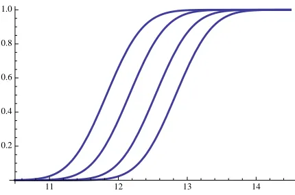
13 14 15 16 17 18 0.2
0.4 0.6 0.8 1.0
Fig. 1.Stage 2.1 for the (128,8)-setting: success rate over an increasing number of leakage traces (in log2-scale) for a computing power of 2k with k ∈
{0,1,8,32}.
11 12 13 14
0.2 0.4 0.6 0.8 1.0
Fig. 2.Stage 2.1 for the (64,4)-setting: success rate of stage 2.1 over an increasing number of leakage traces (in log2-scale) for a computing power of 2k withk ∈
{0,1,8,32}.
Stage 2.1. For this stage (recovery of λ, k2,S(0), S(1), . . . , S(s−1)) we fixed the number s of s-box outputs in the system to 14 for the (128,8)-setting and to 10 for the (64,4)-setting (according to the suggested formulas=n+2−32/m). For both settings, we chose a precision quality parameterq = 0.5 for the building of the template basis and we simulated the attack for a computing power of 2k with k ∈ {0,8,16,32} (i.e. 2k systems among the likeliest ones
are tested). The obtained success rates are plotted in Figure 1 for the (128,8)-setting and in Figure 2 for the (64,4)-setting. Each curve represents a different computing power. Naturally the leftmost curves (i.e. the most successful) correspond to the 232 computing power and
the rightmost ones to the 20 computing power. As one can see, with a reasonable computing
power, a 100% success rate is reached with less than 216leakage traces for the (128,8)-setting, and with less than 213 leakage traces for the (64,4)-setting.
13.5 14.0 14.5 15.0
0.2 0.4 0.6 0.8 1.0
Fig. 3.Stage 2.1 for the (128,8)-setting: success rate over an increasing number of leakage measurements (in log2-scale) for a estimation qualityq= 0.1.
11.5 12.0 12.5 13.0
0.2 0.4 0.6 0.8 1.0
For the (128,8)-setting the precision quality q = 0.5 makes our means estimations to converge after 1024 leakage samples per value β ∈ F256. Since 16 samples are provided per leakage trace (one for each s-box in the first round), this makes a data complexity of 214 leakage traces for building the template basis. As we need around 216 leakage traces to get a
100% success rate in stage 2.1 we might get a better overall attack complexity by improving the estimation precision a little bit. In order to see the kind of improvement we could get from a better estimation, we also performed attack simulations for a precision quality q = 0.1, implying an increase of the data complexity to 217 leakage traces for the template basis. The
obtained success rates are given in Figure 3. We get a 100% success rate with between 214 and 214.5 leakage traces for all computing powers except for k= 0 which requires 215 traces. For the (64,4)-setting, the estimated means converge after 2048 samples per value β ∈
F16, making a data complexity of 2048 for template basis. Here again we also performed
attack simulations for a precision quality of q= 0.1 (see results in Figure 4). We get a data complexity of 213leakage traces for the template basis and around 212.5 leakage traces for the
system solving. This precision therefore seems to give the best tradeoff for the (64,4)-setting.
0.2 0.4 0.6 0.8 1.0
5000 10 000 15 000
Fig. 5.Number of leakage traces to get a 90% success rate over an increasing SNR in [0.1; 1] for the (128,8)-setting (green curve) and the (64,4)-setting (red curve).
In order to observe the impact of the SNR on the data complexity we performed attack simulation for which we weighted the noise covariance matrix in order to get some desired multivariate SNR between 0.1 and 1. For both settings, we fixed the estimation quality to
q= 0.5 and the computed power to 216. Figure 5 plot the required number of leakage traces
to obtain a 90% success rate with respect to the multivariate SNR. We observe a strong impact of the SNR on the attack efficiency. In particular for an SNR close to 1 our attack only requires a few thousands of traces.
Stage 2.2 and 3. The recovery of the remaining s-box outputs based on the maximum
and reaches a 97% success rate for the (128,8)-setting (a tighter likelihood bound would yield a 100% success rate). For the (64,4)-setting, it stops after 10 leakage traces on average and reaches a 100% success rate. The high efficiency of the attack for the (64,4)-setting comes from the fact that it only has to recover 6 remaining s-box outputs. Therefore the likelihoods quickly converge.
We did not implement attack simulation for the third step but we would clearly get comparable figures than for stage 2.2, i.e. negligible data requirements compared to stage 2.1 which is clearly the bottleneck of our attack.
8
Discussions and Perspectives
In this paper we have described a generic SCARE attack against a wide class of SPN block ciphers. The attacker model defined in Section 3.1 assumes that colliding s-box computations can be detected from the side-channel leakage. We have first investigated the case of perfect collision detection and then we have extended our attack to deal with noisy leakages.
About the attacker model. As mentioned in Section 3.1 (Remark 2), our attacker model
implicitly means that the cipher implementation processes the s-box computations in a sequential way, which is therefore more suited for software implementations. This makes sense for secret ciphers which are rarely implemented at the hardware level. Note that it is also common to use a sequential approach for the s-box computations in light-weight hardware implementations of block ciphers, and our attack naturally applies to this context. Our model further implicitly assumes that two s-box computations with the same input at two different points in the execution produce identical side-channel leakages (or identically distributed in the noisy context). Although this assumption seems fair in practice, it might not always be satisfied. It was for instance observed in [18, 30] that for some software implementations the side-channel leakage of an s-box computation may vary according to the s-box index and the target register. For such implementations, it might not be possible to detect collisions between two s-box computations at different indices. This issue can be addressed by considering each s-box index independently, which amounts to deal with the multiple s-boxes setting studied in Section 4.1 (except that we need to recover a single s-box). In this context, one only detects collisions between s-box computations at the same index. Note that our attack still assumes that s-box computations at a given index leak identically in the successive rounds.
Countermeasures to our attack. Our work shows that under a practically relevant
collisions. In a variant of their attack against AES-like secret ciphers, Clavieret al. take this constraint into account in order to bypass the masking countermeasure with table recom-putation [13]. Our attack in the idealized leakage model (perfect collision detection) could also be extended to work with this constraint. It would be more tricky in the presence of noise as averaging would not be an option anymore, but our attack could still be generalized using a similar approach as [30]. In order to thwart our attack, one should therefore favor masking schemes enabling the use of different masks for the different s-box computations (see for instance [9, 27]), so that intra-execution collisions would not be detectable anymore. Another common software countermeasure is operation shuffling (see for instance [23]). This countermeasure has a direct impact on our attack as it randomizes the indices of the s-box computations from one execution to another. As shown by Clavier et al. [13], such a coun-termeasure can be simply bypassed in the idealized leakage model. However, it seems more complicated to deal with in a noisy leakage model especially if combined with masking. We therefore suggest to use such a combination of countermeasure against our attack.
Perspectives. Our work opens several interesting issues for further research. First, our attack could probably be improved by using better/optimal approaches to solve the set of noisy equations arising in Stage 2.1 (see Section 6.2). One could for instance follow the ap-proach of [17, 19] by rewriting the system as a decoding problem. Our attack could also be improved by considering a known ciphertext scenario (as e.g. done in [13]). On the other hand, our attack was only validated by simulations (although from a practically inferred leakage model). It would be interesting to mount the attack against a real implementation of a secret SPN cipher e.g. on a smart card, to check how the different steps work in prac-tice. Another interesting direction would be to investigate extensions of our attack against protected implementations in order to determine to what extent an implementation should be protected in practice.
Acknowledgements
This work has been financially supported by the French national FUI12 project MARSHAL+ (Mechanisms Against Reverse-Engineering for Secure Hardware and Algorithms). We would like to thank Victor Lomn´e for providing the microcontroller side-channel traces and the anonymous reviewers for their useful comments.
References
1. Mehdi-Laurent Akkar and C. Giraud. An Implementation of DES and AES, Secure against Some Attacks. In C¸ .K. Ko¸c, D. Naccache, and C. Paar, editors, Cryptographic Hardware and Embedded Systems – CHES 2001, volume 2162 ofLecture Notes in Computer Science, pages 309–318. Springer, 2001.
2. Amir Bennatan and David Burshtein. Design and Analysis of Nonbinary LDPC Codes for Arbitrary Discrete-Memoryless Channels. IEEE Transactions on Information Theory, 52(2):549–583, 2006.
![Fig. 5. Number of leakage traces to get a 90% success rateover an increasing SNR in [0.1; 1] for the (128,8)-setting(green curve) and the (64,4)-setting (red curve).](https://thumb-us.123doks.com/thumbv2/123dok_us/7900468.1311478/24.612.189.426.313.455/number-leakage-traces-success-rateover-increasing-setting-setting.webp)