The Development of a 1-D Integrated Hydro-Mechanical Model Based on Flume Tests, to Unravel Different Hydrological Triggering Processes of Debris Flows

Article

1

The development of a 1-D integrated

hydro-2

mechanical model based on flume tests, to unravel

3

different hydrological triggering processes of debris

4

flows

5

Theo W.J. van Asch 1,2_{, Bin Yu} 2 _{, Wei Hu} 2

6

1. _{Faculty of Geosciences, Utrecht University, P.O. Box 80115, 3508 TC, Utrecht, the Netherlands.}

7

2. _{State Key Laboratory of Geohazard Prevention and Geoenvironment Protection, Chengdu University of}

8

Technology, Chengdu, Sichuan, 610059, P.R. China; [email protected] ; [email protected].

9

* Corresponding author: Th.W.J. van Asch Nachtegaalstraat 6 4116 BP Buren The Netherlands;

10

[email protected]: 00 31 344 571449

11

12

Abstract: Many studies, which try to analyze conditions for debris flow development, ignore

13

the type of initiation. Therefore this paper deals with the following questions: What type of

hydro-14

mechanical triggering mechanisms for debris flows can we distinguish in upstream channels of

15

debris flow prone gullies? Which are the main parameters controlling the type and temporal

16

sequence of these triggering processes and what is their influence on the meteorological thresholds

17

for debris flow initiation? A series of laboratory experiments were carried out in a flume, 8 m long

18

and with a width of 0.3 m. to detect the conditions for different types of triggering mechanisms. The

19

flume experiments show a sequence of hydrological processes triggering debris flows, namely

20

erosion and transport by intensive overland flow and by infiltrating water causing failure of

21

channel bed material. On the basis of these experiments an integrated hydro-mechanical model was

22

developed, which describes Hortonian and Saturation overland flow, maximum sediment

23

transport, through flow and failure of bed material. The model was calibrated and validated using

24

process indicator values measured during the experiments in the flume. Virtual model simulations,

25

carried out in a schematic hypothetical source area of a catchment show that slope angle and

26

hydraulic conductivity of the bed material determine the type and sequence of these triggering

27

processes. It was also clearly demonstrated that the type of hydrological triggering process and the

28

influencing geometrical and hydro-mechanical parameters may have a great influence on rainfall

29

intensity-duration threshold curves for the start of debris flows.

30

Keywords: triggering of debris flows; overland flow; infiltration; laboratory experiments;

31

modelling; rain intensity-duration threshold curves.

32

33

1 Introduction

34

A debris flow is one of the most dangerous types of mass movement because depending on the

35

rheology and topography it can reach a very high speed and large run-out distance. Important

36

study aspects are the mechanism and boundary condition of the initiation process of a debris flow,

37

because it determines the meteorological threshold conditions and further evolution and it will

38

provide clues for future mitigation strategies [1].

39

One can make different classifications of initiation mechanisms based on different viewpoints

40

[1] It was among others [2-3], who stressed the importance of the infiltration capacity of the soil as a

41

key factor for either the development of shallow landslides or surficial erosion and transport of

42

material by overland flow, that might create different types of flow like mass movements. Effective

43

overland flow driven triggering processes are mainly concentrated in channels where high water

44

discharges, severe erosion and transport lead to high solid concentrations generating debris flows

45

[4-9]. Material is supplied to these debris flows by detachment and transport of the bed material but

46

also through lateral erosion of the channel bed. The channel can be partly or totally blocked by

47

landslide dams. High run off discharges eroding these landslide dams can also lead to initiation

48

and rapid grow of debris flows ([10-12]. Landslide damming can also be initiated by rapid incision

49

of the channel bed destabilizing the side walls [13]. With infiltrating driven triggering mechanisms,

50

shallow landslides are generated, which may or may not transform into debris flows. This failure

51

mechanism by infiltrating water can occur in channel beds filled with loose material [14] and on

52

planar slopes where shallow landslides can also transform into debris flows [15-18]. The

53

transformation of a failed mass into a debris flow is rather complex and depends on various

hydro-54

mechanical processes related to pore pressure development and supply of abundant overland flow

55

water further mobilizing the failed mass ([19-23].

56

Several authors analyzed partly the role of hydro-mechanical and morphometric factors

57

controlling the type of initiation of debris flows. Berti [24] analyzed the hydrological factors for the

58

generation of debris flows in typical source areas in the Italian Alps by modelling channel overland

59

in the channel bed from a source area as a response to rainfall impulses. Kean [25] proposed an

60

integrated hydro-geotechnical dynamic model to describe sediment transport by overland flow and

61

consequent mass failure transforming into debris flow surges. Hu [26] highlighted the initial soil

62

moisture and thus infiltration capacity as a controlling factor for the type of initiation: wet soils

63

created mainly surficial run-off and erosion and incision, bank failure, damming and debris flow

64

development while dry soils showed mainly infiltration and landslide failure and debris flow

65

initiation .[1] Zhuang focused more on the slope gradient as a controlling factor for different types

66

of initiation. Their flume studies revealed that at gentler slope gradients around 100 _{± 2}0 _{, incision}

67

and bank failure is dominant, creating channel damming and dam failure, inducing debris flows.

68

At intermediate slopes around 150 _{± 3}0 _{erosion of bed material occur at high discharges. The high}

69

sediment transport capacity with high sediment concentrations is sufficient to create debris flows.

70

At steeper slopes around 210_{± 4}0 _{bed failure by infiltrating overland flow water with debris flow}

71

formation is the most dominant process.

72

Meteorological thresholds for the initiation of debris flows are closely related to the process of

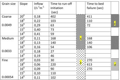
73

initiation. In many studies about these meteorological thresholds, no clear distinction was made

74

between the types of triggering ([27]. The assessment of these thresholds in relation to various

75

morphometric and geological factors was made in most cases using statistical techniques [28-30].

76

Until now only isolated aspects of the hydrological triggering system of debris flows has been

77

studied. There is a need for a comprehensive frame work which gives insight in the controlling

78

factors for the evolution of different triggering systems in upstream channels of debris flow gullies.

79

Therefore this paper will try to give answers on the following questions:

80

1. What type of hydro-mechanical triggering mechanisms for debris flows can we

81

distinguish in upstream channels of debris flow prone gullies?

82

2. Which are the main parameters and in what way are they controlling the type and

83

temporal sequence of these triggering processes?

84

3. What is the influence of hydro-mechanical parameters and related triggering processes

85

on the meteorological thresholds for debris flow initiation?

86

In order to answer these questions we have carried out a number of flume tests to detect the

87

conditions for different types of hydro-mechanical triggering mechanisms of debris flows (Section

88

2). Based on the process information revealed by these experiments we will develop an integrated

89

hydro-mechanical model describing these triggering processes (Section 3). The model will be

90

calibrated and validated using indicator values obtained from the processes measured in the flume

91

(Section 4). Virtual model simulations will be carried out in a schematic hypothetical source area of

92

a catchment to make a frame work of the type and sequence of these triggering processes as a

93

function of slope angle and the hydraulic conductivity of the bed material (Section 5). The model

94

will also be used for sensitivity analyses to study the influence of important geometrical and

hydro-95

mechanical parameters and the related type of initiation process on rainfall intensity-duration

96

threshold curves, for the start of debris flows (Section 6).

98

99

.

2 Flume tests to reveal types of debris flow triggering

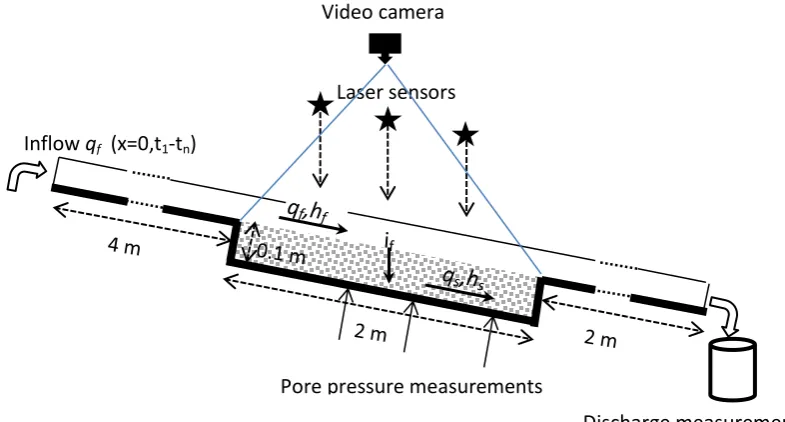
2.1 Set up of the flume experiments

100

A flume was designed to see whether we could simulate in an1D frame work the initiation of

101

debris flows by different hydro-mechanical triggering mechanisms. (Figure 1). The flume has a

102

length of 8 m and a width of 0.3 m. The material simulating the channel bed with a thickness of 0.1

103

m and a width of 0.3 m is positioned at a distance of 4 m from the top of the flume and has a length

104

of 2 m. The material was brought into the flume in layers of about 2 cm and was slightly compacted

105

(dry density see Table1). There is an outflow at a distance of 2 m from the lower end of the channel

106

bed (Figure 1). The water is entered at the upper end of the flume with a controlled discharge

107

,simulating run on water from an upstream area.

108

Figure 1: Design of the flume test. For explanation of the parameters see text

109

Particle size class

Friction

(o₎

Densit y

kNm-3

Hydraulic

conductivity (m s-1₎

D30 (mm) D50 (mm)

D90 (mm)

Coarse 34.6 15.4 4.91E-03 9 11 18

Medium 33.7 16.3 3.28E-03 4 6 16

Fine 29.2 19.5 0.54E-03 0.7 1.6 8

Table I. Hydro-mechanical characteristics of three types of bed material, used in the flume tests.

110

Friction means friction angle of the material in degrees. D30/50 means that 30/50% of the sample has a

111

lower diameter than what is indicated in the column.

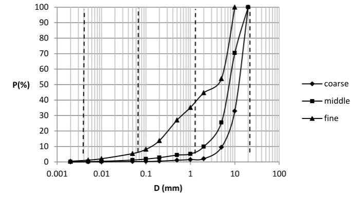
112

Three types of material were used in the experiments with different grain size distributions

113

(Figure 2). We could vary the slope angle of the flume between 140 _{and 20}0_{. The initial moisture}

114

content of the flume material was more or less dry. The initial moisture content is important for the

115

infiltration capacity but since we used in the laboratory a large influx of water from above into

116

coarse bed material, we ignored the effect of the Sorpetivity (related to the initial moisture content)

117

on the infiltration capacity of the bed material.

118

Inflow

q

-t

)

Discharge measurements

Pore pressure measurements

119

Figure 2: Cumulative grain size distribution of the three bed materials, used in the flume tests

120

The friction of the three materials was measured with the conventional direct shear apparatus

121

[31]. The hydraulic conductivity of saturated cylindrical soil samples of the three grainsizes was

122

measured with a constant head gradient between the upper and lower end of the sample ([32].

123

Table I gives further information about the friction, hydraulic conductivity and gradient of the

124

materials used for the experiments.

125

Pore pressure was measured at three places (Figure 1) at the bottom of the flume. The pore

126

pressure sensors, type :YP4049, were produced by Yom Technology Company. The measuring

127

range of pore pressure is from -100kPa to +100kPa.

128

Laser sensors (ZLDS100 ZSY Group; resolution 0.03 % FS) at three points with a spacing of 0.5

129

m (Figure 1) were used to monitor topographical heights, especially with the aim to monitor abrupt

130

changes in relief due to bed failure.

131

In addition video-recordings were performed (Figure 1) to follow the sequence of processes in

132

the course of the experiments. During the process of overland flow erosion, samples were taken six

133

times for more or less steady state conditions at the outlet of the Flume (Figure 1). The discharge of

134

water with sediments was collected in baskets during 5 seconds. The sediments were sieved, dried

135

and weighted to measure the concentration of the fluid.

136

An integrated model (Section 3) for surface and sub surface flow, sediment transport and bed

137

slope stability was developed to describe the processes in the flume, which was used later to

138

analyze the sequence of different initiation processes at the field scale.

139

2.2 Observations on different types of hydrological triggering mechanisms in flume tests.

140

The flume tests were carried out in order to reveal different types of hydrological triggering

141

mechanisms, which may create debris flows and to establish indicators related to these triggering

142

processes which will be used to calibrate and validate our theoretical model (Section 4) During the

143

flume tests with the three bed materials under different slope angles, observation were carried out

144

by means of video images and the laser sensors. Some of the observed process indicators are given

145

in Table II

146

147

148

0 10 20 30 40 50 60 70 80 90 100

0.001 0.01 0.1 1 10 100

P(%)

D (mm)

Grain size Slope

Inflow

l/s

m

Time to run-off

initiation

(sec)

Time to bed

failure (sec)

Coarse

0.0049

20

0,18

402

411

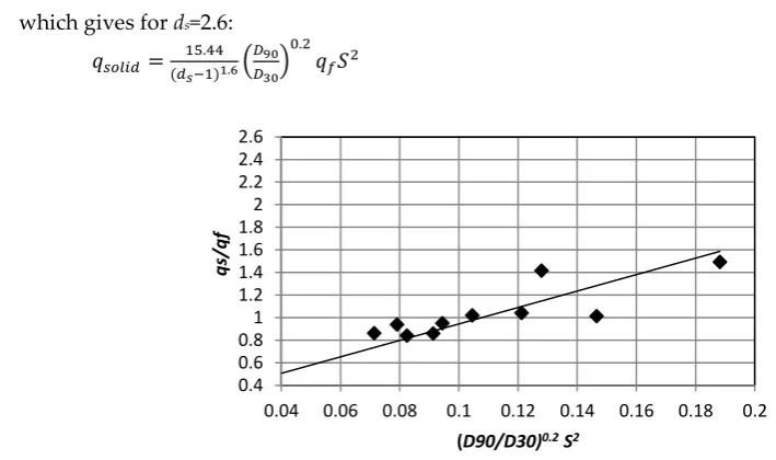
18

0,22

103

110

16

0,29

63

72

15

0,40

73

14

0,41

59

Medium

0.0033

20

0,11

168

168

18

0,13

140

140

16

0,16

54

106

15

0,18

27

14

0,19

46

Fine

0.00054

20

0,03

30

270

18

0,06

220

613

16

0,09

90

270

15

0,10

110

14

0,11

102

149

Table II. Observed time to overland flow and bed failure, overland flow type and failure mode in

150

flume experiments for three types of bed material and for different bed slope angles: a) Saturation

151

overland flow; b) Hortonian overlandflow; c) slow continuous bed failure; d) rapid failure; nf: no

152

failure.

153

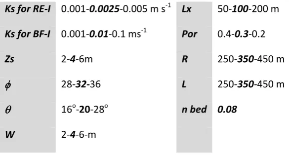
In slope hydrology two types of overland flow can be distinguished: Saturation overland flow

154

and Hortonian overland flow [32]. These two types could be distinguished during the different

155

flume experiments (Table II). Saturation overland flow was characterized, after complete saturation

156

of the soil, by a more or less spatially randomly ponding of water at the soil surface, while

157

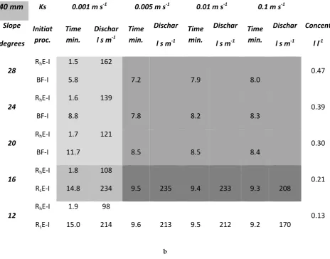
Hortonian overland flow, which occurs when the rainfall intensity or supply of overland flow water

158

is larger than the infiltration capacity of the soil, showed a more concentrated continuous flow over

159

the length of the flume bed. According to these visual indicators we could establish a boundary

160

between Saturation overland flow and Hortonian overland flow, which in our flume tests was

161

found in the medium grain size materials at a slope gradient of 160 _{(Table II). This could be verified}

162

with our model simulation (see below Section 4.2). For courser materials (Ks values of 4.19E-03 and

163

3.28E-03 m s-1 _{) and higher slope angles (> 16}0 _{) the time to Saturation overland flow is immediately}

164

followed by failure or with a small delay until 9 seconds. Also one can clearly observe that the time

165

to Saturation overland flow (and thus failure) is decreasing with decreasing slope angle (Table II) .

166

Hortonian overland flow [32].was initiated in most cases on the finer sediments, which is

167

ascribed to the lower infiltration capacity (Ks = 0.54E-03 m s-1_{). Bed failure in this case occurred a}

168

certain time after the start of Hortonian overland flow with a time lag ranging between 35 and 160

169

seconds (Table II), because in this case, due to the lower percolation rate it takes time to bring the

170

groundwater in the bed material to a critical failure level.

171

Bed failure initiation is controlled by the bed gradient and the internal friction of the material

172

and occurred in our experiments on slopes of approximately 16 degrees and higher. At lower slope

173

angles no bed failure occurred (nf in Table II) and sediment delivery occurred only by overland

174

flow erosion

175

The medium and course materials show bed failure characterized by slow movements over the

176

total depth combined with fast surficial entrainment of grains by saturated overland flow.

177

Movement of bed material is slow and continuous or sometimes intermittent showing a surging

178

a

b

pattern (Table II). Instead of the slow and more flow like movements observed for the medium and

179

coarse sediments, failure of the fine sediments occurred suddenly with a very rapid surge of more

180

or less coherent blocks followed by fluidization, (Table II).

181

Sediment transport by overland flow on these steep slopes reached volumetric concentrations

182

between 0.46 and 0.64, which is characteristic for debris flows

183

184

185

186

187

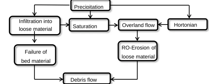
188

Fig 3. Schematic diagram showing the different initiation processes of debris flows in channels

189

We can conclude on the basis of these observations that the flume tests carried out with the

190

three materials revealed three types of processes, which created debris flows in these range of

191

slopes gradients namely debris flow Initiation by Hortonian Overland flow Erosion (RhE-I),

192

Saturation Overland flow Erosion (RsE-I) and by Bed Failure (BF-I). The occurrence and sequence

193

of these processes seems to be controlled by slope gradient and hydraulic conductivity of the bed

194

sediment. Figure 3 gives a schematic overview of these process types.

195

3 Integrated model (1D) for debris flow initiation in upstream channels

196

The flume tests observations brought us to the concept of the triggering of debris flows caused

197

by Hortonion and Saturation overland flow initiating surficial erosion of bed material. Bed failure

198

and entrainment of material was initiated by infiltration and subsurface flow leading to instability.

199

First we have to simulate the hydrological component of the triggering mechanisms of debris flows.

200

For that we need the mass balance equation for overland (Eq.(1a)) and through flow (Eq.(1b)) ,

201

which is given by :

202

𝜕𝑞𝑓

𝜕𝑥 + 𝜕ℎ𝑓

𝜕𝑡 = 𝐵1 (1a)

203

𝜕𝑞𝑠

𝜕𝑥 + 𝜕ℎ𝑠

𝜕𝑡 = 𝐵2 (1b)

204

205

where qf is overland flow discharge per unit width (m3m-1s-1); qs is subsurface discharge per unit

206

width (m3_m-1_s-1_{); hfis thickness of overland flow (m); hs (m) is thickness of subsurface flow, 𝜕x (m) is}

207

distance along the slope 𝜕t is the time (s) and B1-2 are terms (m s-1_{) describing the inflow or outflow}

208

of water from the flow system, which is defined as follows:

209

𝐵1= [

𝑟 − 𝑖𝑓 (𝑎) 0 − 𝑖𝑓 (𝑏)

] (2a)

210

𝐵2= 𝑖𝑓 (2b)

211

212

where r (m s-1_{) describes the external input of rain into and if (m s}-1_{) the outflow of water by}

213

infiltration out of the overland flow system (Eq. (2a)) (see also Figure 1). When there is no supply of

214

rain, like in our flume experiments: r=0. In the case of subsurface flow if in Eq.(2b) is considered

215

now as an inflow term of the subsurface flow system. If hf/t is larger than the infiltration capacity

216

Ks (m s-1_{) of the bed material the latter one is the limiting factor. Therefore the infiltration term if of}

217

Precipitation

Overland flow

RO-Erosion of

loose material

Debris flow

Infiltration into

loose material

Failure of

bed material

-1_{) and the current water depth}

218

(hf), which can infiltrate in one time step t into the bed material:

219

𝑖𝑓 = min (𝐾𝑠, ℎ𝑓/∆𝑡) (3)

220

221

We introduce here a general momentum equation for the water flow processes [33]:

222

ℎ𝑓= 𝛼𝑓𝑞𝑓𝛽𝑓 (4a)

223

ℎ𝑠= 𝛼𝑠𝑞𝑠𝛽𝑠 (4b)

224

225

For turbulent overland flow the parameters fand f in Eq.(4a) can be defined as follows :

226

𝛼𝑓= ( 𝑛 𝑆00.5)

0.6

and 𝛽𝑓 = 0.6 (5)

227

where n is Manning’s n and S0 the slope gradient of the bed material.

228

For subsurface flow we can write according to Darcy’s law:

229

𝑞𝑠= 𝐾𝑠 sin 𝜃 ℎ𝑠→ ℎ𝑠= 1

𝐾𝑠 sin 𝜃𝑞𝑠 (6)

230

231

where qs is the amount of subsurface flow water per unit width (m3m-1s-1); is slope angle (degrees)

232

and hs is the height of the flowing water component in the soil matrix (m). By comparing Eq.(6) with

233

the general momentum Eq. (4b) we can define the parameters

234

sand s for subsurface flow:

235

𝛼𝑠= 1

𝐾𝑠 𝑠𝑖𝑛𝜃 and 𝛽𝑠= 1 (7)

236

237

A combination of the mass balance Eq.(1) with Eq.(4) delivers an expression for overland flow

238

or subsurface flow discharge (qf,qs) [33]:

239

𝜕𝑞_𝑓

𝜕𝑥 + 𝛼𝑓𝛽𝑓𝑞𝑓

(𝛽_𝑓,𝑠−1) 𝜕𝑞𝑓

𝜕𝑡 = 𝐵1 (8a)

240

𝜕𝑞𝑠

𝜕𝑥 + 𝛼𝑠𝛽𝑠𝑞𝑠

(𝛽𝑠−1) 𝜕𝑞𝑠

𝜕𝑡 = 𝐵2 (8b)

241

242

The 1D model is implemented in a fixed Eulerian frame where the variation in water flow

243

variables is described at fixed coordinate points at a distance x along the slope as a function of

244

time step t. A numerical solution for Eq.(8) is given by [33]:

245

𝑞𝑥+1𝑡+1 =

∆𝑡 ∆𝑥𝑞𝑥

𝑡+1_{+𝛼𝛽𝑞} 𝑥+1𝑡 (𝑞𝑥+1

𝑡 _+𝑞𝑥𝑡+1

2 )

𝛽−1

+∆𝑡(𝐵𝑥+1𝑡+1 +𝐵𝑥+1

𝑡

2 )

∆𝑡 ∆𝑥+𝛼𝛽(

𝑞𝑥+1𝑡 +𝑞𝑥𝑡+1

2 )

𝛽−1 (9)

246

247

where qx, and  should be read as qf,s f,s and f,s respectively.

248

To simulate the initiation of debris flows by mass failure we used the equation for the infinite

249

slope equilibrium model [31], which is the trigger for failure:

250

𝐹 =( 𝛾𝑠𝑧 𝑐𝑜𝑠 𝜃−𝑝) 𝑡𝑎𝑛 𝜑

𝛾𝑠𝑧 𝑠𝑖𝑛 𝜃 (10a)

251

𝑝 = 𝛾𝑤ℎ𝑠cos 𝜃 (10b)

252

253

where F is the safety factor; failure occurs when F=1; s and w are the saturated bulk density of the

254

material and water respectively; is friction angle of the material; z and hsare the thickness of the

255

soil and the height of the groundwater layer respectively hs can be solved with Eq. (9) and Eq.(6)

256

respectively.

257

The overall stability of the bed material expressed with the safety factor (F) for the infinite

258

slope model is calculated as an average of the safety factor of the different nodes. The inflow of

259

water into the flume is coming from upstream and therefore the pore pressure gradient is

260

decreasing downstream. This means that the safety factor is always increasing downstream and

261

therefore the average approach of the safety factor over the length of the sample in the flume seems

262

a reasonable approximation of the overall safety factor.

For estimating the transport capacity on steep slopes Rickenmann [34-35] proposed a bedload

264

transport equation based on a shear stress approach, where discharge, bed slope gradient and

265

material grading are used as parameters to characterize flow hydraulics.

266

For steeper slopes, in the range of 0.03<S<0.2 (1.7o_-11.3o_{) Rickenmann [34] performed a}

267

regression analysis with the steep flume data on bed load transport obtained at ETH Zurich that

268

resulted in the equation:

269

𝑞𝑠𝑜𝑙𝑖𝑑= 12.6 (𝑑𝑠−1)1.6(

𝐷₉₀ 𝐷30)

0.2

(𝑞𝑓− 𝑞𝑐)𝑆2 (11)

270

271

where D90 and D30 are grain sizes at which 90% and 30% respectively by weight of the material are

272

finer; dsis the mass density of the solids and S is the slope gradient and qc is the critical flow

273

discharge for bed load entrainment. The experimental slopes were in the range of 0.03>S>0.20. (1.70

-274

11.30_{) and the D90 of the material ranged between 0.9>and2 cm and D30 between 0,06 and 1 cm with}

275

inflow rates of 10-30 l/s In the section below we will calibrate Eq.(11) for the steeper slopes in our

276

flumes.

277

The integrated model developed in this section is able to describe the different types of

hydro-278

mechanical triggering mechanisms for debris flows. It delivers us the physical parameters, which

279

controls these processes, which will be applied in our virtual simulations in Section 5 and 6

280

In the next section (4) we will calibrate our model on some process indicator values obtained from

281

our flume tests.

282

4. Calibration and validation of the theoretical model on the basis of flume test results

283

. We will use here a number of process indicator values measured during the flume

284

experiments to calibrate and validate the outcomes of our theoretical model. These are: Saturation

285

or Hortonian overland flow, time to overland flow, maximum pore pressure, time to bed failure

286

and solid concentration by overland flow erosion. Hortonian overland flow and the time to

287

Hortonian overland flow in the model is declared when surface water hfreaches the lower end of

288

the bed material while the bed material is still not saturated (hs < Zs) .Saturation overland flow and

289

the time towards it, is declared when hs = Zs over the entire bed. Pore pressure is calculated each

290

time step according to Eq (10b). The discharge of hf + hs is reported each time step at the end of the

291

flume. Bed failure is declared as said before when the average Safety factor F over the bed length

292

reaches the value of 1.

293

For the flume simulations the distance between the nodes (x) was 0.1 m and the time interval

294

(t) was 0.2 seconds.

Figure 4. Observed and calculated time to Saturation overland flow (black symbols) and Hortonian

296

overland flow (open symbols)

297

Figure 4 shows the relation between observed and calculated time to overland flow for the

298

different flume tests. There is a moderate 1:1 correlation between observed and predicted time to

299

overland flow for the medium and coarse sediments and for the fine sediments, showing Hortonian

300

overland flow, there is no correlation at all. However the model was able to predict the type of

301

overland flow according to what was observed during the flume tests (see Table II).

302

Despite the malfunctioning of some pore pressure sensors we were able to make a 1:1

303

comparison between the average maximum measured pore pressure for the three sensors (Figure 1)

304

and the average calculated maximum pore pressure (Figure 5).

305

306

Fig 5. Maximum pore pressure measured during flume tests in relation to calculated pore pressures.

307

The Figure shows that in many cases there is a slight overestimation of the calculated pore

308

pressure. Time series of measured pore pressure of the three sensors compared to modelled

309

temporal pore pressure development showed thatin most cases the onset towards maximum pore

310

pressure for the three sensors is more irregular compared to the calculated development of the pore

311

pressures (Figure 6). This can be ascribed to the heterogeneity of the sediment or (and) the

312

imperfect response of the sensors.

313

0 0.2 0.4 0.6 0.8 1 1.2 1.4

0.6 0.7 0.8 0.9 1

p

c

al

cu

late

d

(

kPa)

p measured (kPa)

1:1 line

0 20 40 60 80 100 120 140 160 180

0 50 100 150 200

Ti

m

e

t

o

o

ve

rl

an

d

fl

o

w

b

ser

ve

d

(sec

)

Time to overland flow Calculated (sec)

coarse

medium

314

Fig 6 Example of the rise in pore pressure (measured /calculated) due to infiltration of run-on water

315

in the bed material (Test:Medium grain size /200₎

316

In relation to pore pressure development we compared the time to failure for the different test

317

runs on the different materials. Since the time towards average maximum calculated and measured

318

pore pressure coincided more or less, one would expect also corresponding calculated and

319

measured failure times. Table II and Figure 7 show that the match between observed and calculated

320

failure time is reasonable except for two outliers (coarse-200 _;fine-180_{). Further we can observe that}

321

the calculated time to failure is underestimated for the coarse material and overestimated for

322

practically all the tests on the medium and fine materials. The deviations between calculated and

323

observed values must be ascribed to heterogeneity of the material, deviating friction values, and

324

incorrect assessment of the overall safety factor.

325

326

Figure 7: Observed and calculated time of failure of bed material during the flume tests.

327

We calibrated also the parameters of the Rickenmann [35] equation, (Eq.11) on our flume tests,

328

which were carried out on slopes ranging between 0.25>S>0.36 (140_-200_{), with grain sizes for}

329

0.9>d90>2 and 0,05>d30>1 cm and with flow rates 0,5>qf>15 l s-1 m-1. Figure 8 shows the best linear fit

330

between qsolid/qf and (d90/d30)0.2_S2_{, which delivered the following modified equation for slopes}

331

between 140 _{and 20}0_:

332

𝑞𝑠𝑜𝑙𝑖𝑑 = 7.28 ( 𝐷90

𝐷₃₀) 0.2

𝑞𝑓𝑆2 (12a)

333

0 0.1 0.2 0.3 0.4 0.5 0.6 0.7 0.8

0 50 100 150 200 250 300 350 400 450

Por

e

p

re

ssur

e

kPa

Time seconds

Calculated

Observed

0 100 200 300 400 500 600 700

0 100 200 300 400 500 600 700

Ti

m

e

t

o

fai

lu

re

c

al

cu

late

d

(

s)

Time to failure observed (s)

coarse

medium

which gives for ds=2.6:

334

𝑞𝑠𝑜𝑙𝑖𝑑= 15.44 (𝑑_𝑠−1)1.6(

𝐷90

𝐷₃₀) 0.2

𝑞𝑓𝑆2 (12b)

335

336

Figure.8. Calibration of Rickenmann’s bedload equation for steeper slopes in our flume tests

337

between 14 and 20 degrees.

338

The calibration revealed that qc in Eq.(11) becomes zero or practical zero in Eq.(12). At slopes

339

larger than 150 _{the down slope component of the grain weight may reduce the critical shear stress} c

340

which in our case obviously reduced to nearly zero.

341

We may conclude that the model is able to predict in a reasonable way essential process

342

indicators for different hydrological triggering processes of debris flows in upstream channels. In

343

the next section we will apply the model on the field scale to predict hydro-mechanical triggering

344

patterns for debris flows as a function of the hydrological conductivity of the bed material and the

345

channel slope gradient.

346

5. Hydro-mechanical triggering patterns for debris flows in relation to hydrologic conductivity

347

of bed materials and channel gradient

348

5.1. The design of a schematic source area at the field scale.

349

First we will design a virtual landscape of a potential debris flow source area where our model

350

can be applied to analyze the influence of terrain parameters on the type of triggering mechanisms

351

(Section 5.2) and the meteorological thresholds of debris flows (Section 6).

352

Figure 9 shows this virtual source area, which is linked to an upstream channel filled with bed

353

material receiving surface water from the surrounding slopes to initiate a potential debris flow. This

354

geomorphological setting resembles more or less the source areas described among others by Coe

355

[7] and Berti [24]. The upstream area of our hypothetical catchment has a radius R. The channel is

356

further surrounded by lateral slopes with a length L. The length of the channel bed is Lx , the width

357

W and the slope angle is  .The hydraulic conductivity of the bed material is Ks, the porosity Por

358

and the friction angle . (Figure 9).

359

0.4 0.6 0.8 1 1.2 1.4 1.6 1.8 2 2.2 2.4 2.6

0.04 0.06 0.08 0.1 0.12 0.14 0.16 0.18 0.2

qs/qf

360

Figure 9: Morphometric and hydro-mechanical parameters, which were used for model simulations

361

of debris flow initiation. For an explanation see Table 3 and text. D90/D30: 90% and 30% lower than

362

grainsize D90 and D30 respectively :





363

depth of material; : slope angle, qup: water that flows into the upper end of the channel bed; R:

364

radius of source area above the channel; Lx and W: length and width of the channel bed; L: length of

365

lateral contributing slope; latin: lateral inflow of water to the channel; CN: curve number value for

366

the soil hydrological and land use characteristics of the contributing slopes.

367

The sink term B in (1) and (8) is now adapted to the field scene and given by:

368

𝐵 = 2𝑙𝑎𝑡𝑖𝑛 + 𝑟 − 𝑖𝑓 (13)

369

370

where latin (m s-1_{) is the lateral inflow of overland flow water from the slopes along the channel}

371

(Figure 9) , r direct rain intensity input to the channel bed and ifinfiltration rate into the bed (see

372

Eq.(3)). The lateral inflow is calculated for these sensitivity analyses in a simple way, assuming

373

steady state conditions in the mass balance equation for overland flow:

374

𝑙𝑎𝑡𝑖𝑛 =𝑟𝑐𝑛𝐿

𝑊 (14)

375

376

rcn (m/s) is calculated using the Curve Number method [36], L is the length of the lateral slope

377

and W the width of the channel (see Figure 9). In our simulations we selected overland flow

378

supplying slopes with soils with moderate to slow infiltration rates and a poor condition grass

379

cover, which corresponds to a Curve Number(CN) of about 80. The CN number, reflecting the

380

hydrological soil characteristics, land use and antecedent soil moisture conditions that we can

381

expect in high mountainous areas, was chosen arbitrarily and was kept constant in our simulations.

382

The overland flow water that flows into the upper end of the channel bed, which is given by qup (m2

383

s-1_{) (Figure 9)}

384

𝑞𝑢𝑝=

𝑟𝑐𝑛0.5𝜋𝑅2𝑐𝑜𝑠𝜃

𝑊 (15)

385

5.2 The influence of the hydraulic conductivity (Ks) and slope () of the channel bed on the type and sequence

386

of hydrologic triggering processes for debris flows

387

In the flume we could observe the effect of slope angle and hydraulic conductivity on the type

388

and sequence of triggering processes, which may lead to the initiation of debris flows. In this

389

section we will investigate with our theoretical model the effect of these two factors at the

390

catchment scale. The values of the other factors used in our model simulations are shown in bold as

391

default parametric values (Zs,,W,Lx,Por.R.L,n bed) in Table III (see also Figure 9).

Ks for RE-I

0.001-0.0025-0.005 m s

Lx

50-100-200 m

Ks for BF-I

0.001-0.01-0.1 ms

Por

0.4-0.3-0.2

Zs

2-4-6m

R

250-350-450 m



28-32-36

L

250-350-450 m



16

-20-28

n bed 0.08

W

2-4-6-m

Table III. Default values (bold italic) and maximum and minimum values of input parameters for

394

Overland flow Erosion (RE-I) and Bed Failure (BF-I) triggering debris flows. Ks: saturated hydraulic

395

conductivity; Zs: thickness of bed material;friction angle of material; slope angle of channel

396

bed; W and Lx :width and length of channel bed respectively; Por: available volumetric pore space;

397

R radius of source area ; L: length of lateral slopes ; n: Manning’s n of bed material.

398

Table IV gives the range in Ks values (first row) and bed slope angles (first column), which

399

were used in our simulations to study the effect of these parameters on the hydro-mechanical

400

process development at the catchment scale. For these simulations two rain scenarios were used

401

with an intensity of 80 mm (Table IVa) and 40 mm per hour (Table IVb) respectively. The Tables

402

show domains with different shades of gray with various combinations of hydro-mechanical

403

triggering processes. In the white sections no debris flow initiation is expected to develop in the

404

source area because of a too low sediment concentration of the overland flow. Table IVa shows that

405

in the domain  280_-200 _{and Ks= 0.001-0.005 m s}-1_{, the debris flow is initiated in the first stage by}

406

Hortonian overland flow erosion (RhE-I). The overland flow discharge reaches a steady state after a

407

certain relatively short time. During the steady state groundwater will rise by infiltration of run-on

408

water until failure of the bed material, which happens between 1.7 and 11.2 minutes depending on

409

the slope and Ks. In Table IVa we see a dramatic drop in discharge between slopes with Ks =0.001

410

and 0.005. The last Ks-value reaches a significant boundary which determines whether or not a

411

debris flow can be initiated by Hortonian overland flow transport.

412

80 mm

Ks

0.001 m s

0.005 m s

0.01 m s

0.1 m s

Slope

degrees

Initiat

proc.

Time

min.

Dischar

l s m

Time

min.

Dischar

l s m

Time

min.

Dischar

l s m

Time

min.

Dischar

l s m

Concent

l l

28

R

E-I

BF-I

1.0

5.4

912

1.3

1.7

139

2.4

3.0

0.47

24

R

E-I

BF-I

1.0

8.4

783

1.3

2.3

119

2.8

3.1

0.39

20

R

E-I

BF-I

1.1

11.2

683

1.4

2.9

104

3.1

3.1

0.30

16

R

E-I

R

E-I

1.1

14.2

606

732

1.5

3.7

92

733

3.7

732

3.6

705

0.21

12

R

E-I

R

E-I

1.2

14.8

550

666

1.5

3.9

83

665

3.8

664

3.6

646

0.13

a

414

40 mm

Ks

0.001 m s

0.005 m s

0.01 m s

0.1 m s

Slope

degrees

Initiat

proc.

Time

min.

Dischar

l s m

Time

min.

Dischar

l s m

Time

min.

Dischar

l s m

Time

min.

Dischar

l s m

Concent

l l

28

R

E-I

BF-I

1.5

5.8

162

7.2

7.9

8.0

0.47

24

R

E-I

BF-I

1.6

8.8

139

7.8

8.2

8.3

0.39

20

R

E-I

BF-I

1.7

11.7

121

8.5

8.5

8.4

0.30

16

R

E-I

R

E-I

1.8

14.8

108

234

9.5

235

9.4

233

9.3

208

0.21

12

R

E-I

R

E-I

1.9

15.0

98

214

9.6

213

9.5

212

9.2

170

0.13

b

416

Table IV. Time sequence of different initiation processes RhE-I and RsE-I,(erosion by Hortonian and

417

Saturation overland flow respectively) and BF-I (bed failure) in relation with hydraulic conductivity

418

(Ks) and slope angle of bed material. Further are given the discharge (Discharg) and solid

419

concentration (Concent) during RhE-I and RsE-I. Table 4a and 4b: simulated rain intensities of 80 mm

420

and 40 mm respectively.

421

It is confirmed by Table IVb with a lower rain input (40 mm) where at Ks ≥ 0.005, no initiation

422

by Hortonian overland flow is possible anymore.

423

Going back to Table IV-a: in the domain 160_-120 _{and Ks= 0.001-0.005 ms}-1 _{slope failure does}

424

not occur. The debris flow is initiated by overland flow. First by Hortonian overland flow and later

425

when the groundwater has reached the surface by Saturation overland flow. Discharge is relatively

426

low when there is Hortonian overland flow, while obviously discharge dramatically increases at

427

Saturation overland flow. However due to the lower slope angles, the volumetric sediment

428

concentration is low (0.21 at 160 _{and 0.13 at 12}0_{, (Table IV-a last column ), which means the flow}

429

changes from a hyper concentrated flow into a water flood with conventional suspended load and

430

bed load.

431

At higher conductivities in the domain Ks=0.01-0.1 m/s and 28o_-20o_{, bed failure seems the}

432

most dominant process (Table IVa). Due to the larger Ks values, infiltration into the bed is more

433

important than overland flow discharge. The bed material turns out to be partly saturated in the

434

upper part due to the larger upstream inflow, creating partly Saturation overland flow and

435

Hortonian overland flow. However within one minute after the run off discharge reached the lower

436

end of the bed, failure of the bed material occurred already. Therefore the contribution of overland

437

flow to the transport of debris by overland flow can be ignored.

In the domain Ks=0.01-0.1 m/s and lower slope gradients (16o_-12o _{) there is no slope failure}

439

but only Saturation overland flow, (Table IVa ) with low sediment concentrations in most cases not

440

enough to call it a debris flow.

441

Table IV-b shows the simulation results with an intensity of 40 mm per hour. The domains

442

with a specific combination of hydro-mechanical triggers still exist. There is only a shift of the

443

boundary for the Ks -values with no Hortonian overland flow (>0.005 m/s) to the left. The Tables

444

IVa and b show a decrease in overland flow discharge and increase in time to bed failure with a

445

decreasing slope angle. Around 16 degrees the channel bed is stable but still steep enough to have

446

transport capacities with concentrations in the domain of a hyper concentrated flow. These are

447

induced by Hortonian and Saturation overland flow at lower Ks values and only Saturation

448

overland flow at higher Ks values. At lower slope angles (see slopes around 12 degrees) sediment

449

concentrations are too low to call it a debris flow. Table V gives a summary of the type and

450

sequence of initiation processes related to different Ks and slope angle values.

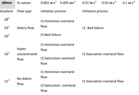
451

40mm

Ks values

0.001

m s

0.005

ms

0.01

m s

0.05

m s

0.1

m s

Gradient Flow type

Initiation process

Initiation process

28

Debris flow

t1:Hortonian overland

flow

t2:Bed failure

t1: Bed failure

24

20

16

Hyper

concentrated

flow

t1:Hortonian overland

flow

t2:Saturation overland

flow

t1:Saturation overland flow

12

No debris

flow

t1:Hortonian overland

flow

t2:Saturation overland

flow

t1:Saturation overland flow

Table V: Sequence of different initiation processes for debris (hyper concentrated) flows in relation

452

to the hydraulic conductivity and slope of the channel bed material. Simulated rain intensity is 40

453

mm.

454

We designed a framework, which gives insight in what kind of debris flow initiation can be

455

expected for a given slope gradient and hydraulic conductivity of the material. In the next section

456

we will give an impression how different hydro-mechanical parameters of triggering processes can

457

influence meteorological thresholds for debris flows..

458

459

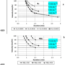
460

462

463

6. Sensitivity analyses for parameters influencing the rain Intensity-Duration (I-D) threshold

464

curves for different initiation processes of debris flows

465

In the foregoing we revealed the influence of Ks and bed slope gradient on the sequence of

466

processes mechanisms involved in the initiation of debris flows. We want to investigate here the

467

effect of the other parameters (including Ks and slope gradient) on rainfall thresholds in terms of

468

Intensity Duration (I-D) curves for the triggering of debris flows by two main process mechanism:

469

initiation by Hortonian overlandflow (RhE-I) and bed failure (BF-I). As we have seen in Table IV

470

and V, debris flow initiation by Saturation overland flow (RsE-I) can only take place around 16

471

degrees At lower slope angles sediment concentrations are too low to call it a debris flow (Table IV).

472

At higher slope angles we have bed failure before Saturation overland flow can take place.

473

Figure 10 shows the effect of different parameters on the I-D curves for debris flows initiated

474

by Hortonian overland flow. The intensity and duration value of a rain event which creates

475

overland flow that just reaches the end of the channel bed with a sediment concentration of >0.2, is

476

defined by us as a threshold rain event for debris flow initiation. The intensity and duration values

477

for a variety of different critical rain events were plotted in a graph with on the y-axis the intensity

478

and on x-axis the duration. In this way an Intensity Duration (ID) curve can be constructed. Table

479

III gives an overview of the range of the different parameters and the default values (in bold italic),

480

which were used in the simulation and which give a realistic representation of geometric and

481

geotechnical parameters for source area conditions The threshold curves for debris flow initiation

482

by Hortonian overland flow are shown in Figure 10. In this figure the threshold curves, which are

483

constructed, using the default values given in table III, are depicted with open rectangular markers.

484

They are equal in all the sub-figures. This enables one to compare for the different parameters the

485

difference between the ultimate curves and the default curve. For each selected parametric value

486

there is an ultimate minimum rain intensity below which not enough overland flow and thus a

487

debris flow can be initiated, irrespective

488

489

490

0 20 40 60 80 100

0.5 1 1.5 2 2.5 3

In

te

nsi

ty

(m

m

/hr

)

Duration (min)

Ks

Ks=0.0005 Ks=0.0010 Ks=0.0050 Ks=0.0025

0 20 40 60 80 100

0.5 1 1.5 2 2.5 3

In

te

n

si

ty

(m

m

/hr

)

Duration ( min) R&L

R&L=250 R&L=350 R&L=450

a

b

0204060 80100 0.511.522.53

Intensity (mm/hr)

Duration ( min) R&L R&L=250R&L=350R&L=450

Y=102.8x-0.9 Y=92.8x-1.2 Y=81.6x-1.1 Y=81.9x-1.3

491

492

493

494

Figure 10. I-D curves for debris flow initiation by Hortonian overland flow in relation to different

495

geometrical and hydrological parameters. For the definition of parameters see Table III.

496

the duration (D) of the rain event (see horizontal dotted lines). The simulations show that at

497

intensities below this critical dotted line the overland flow water never reach the lower end of the

498

bed due to a too high infiltration rate on its pathway compared to the supplied amount of water (

499

direct rain input and surrounding overland flow) and finally bed failure may be the primary

500

triggering process.

501

The most obvious selected parameter for overland flow initiation is the hydraulic conductivity

502

Ks . Other parameters are related to geometry of the source area (see Figure 6) like length of the

503

0.5 1 1.5 2 2.5 3

In te n si ty (m m /hr )

Duration ( min)



16 20 28

0 20 40 60 80 100

0.5 1 1.5 2 2.5 3

In te n si ty (m m /hr )

Duration ( min)

Lx

Lx=50 Lx=100 Lx=200

0 20 40 60 80 100

0.5 1 1.5 2 2.5 3

In te n si ty (m m /hr )

Duration ( min)

n

n=0.06 n=0.08 n=0.10

0 20 40 60 80 100

0.5 1 1.5 2 2.5 3

In te n si ty (m m /hr )

Duration ( min)

W

W=2 W=4 W=6

c

f

0

20

40

60

80

100

0.5

1

1.5

2

2.5

3

I

D

W

d

e

0

20

40

60

80

100

0.5

1

1.5

2

2.5

3

I

D

n

0

20

40

60

80

100

0.5

1

1.5

2

2.5

3

I

D

n

Intensity (mm/hr)

Duration ( min)

lateral slopes along the channel (L ), radius of the upstream area of the channel (R) Length (Lx) and

504

width (W) of the channel bed , channel bed gradient ( and further Manning’s n of the bed

505

material.

506

We saw in the forgoing that Hortonian overland flow plays a dominant role for Ks values <

507

0.005 m s-1_{. Figure 10 a shows the influence of the Ks value on the I-D threshold curves for run off}

508

erosion initiation (RhE-I). The range of Ks values is chosen between 0.0005 and 0.005 m s-1 The

509

Figure shows that for Ks values lower than 0.001 m s-1 _{there is nearly no effect of Ks on the position}

510

of the I-D curve but there is a difference in the minimum intensity values (dotted lines) below

511

which no debris flow can occur. A slight difference can be observed for lower intensities (<60 mm

512

hr-1_).._{Higher Ks values (> 0.001 m s}-1_{) have a larger influence on the I-D curves. (Figure 10a)}

513

The simulations show that the scale of the source area and lateral slopes (R&L), the length of

514

the river bed (Lx) and the width of the bed (W) have the largest effect on the position of the

515

threshold curve for the initiation of debris flow by Hortonian overland flow (Figure 10 b,d,f

516

respectively). The threshold curves are less sensible for the effect of the slope gradient and

517

Manning’s n of the bed material (Figure 10 c,e respectively).

518

519

520

521

522

y = 171.0x-0.6

0 20 40 60 80 100

0 5 10 15 20 25 30 35 40 45 50 55 60 65 70 75 80

In

te

n

si

ty

(m

m

/hr

)

Duration ( min)

Ks

Ks=0,001m/s Ks=0,01 ms-1 Ks=0,1 m/s

y = 236.1x-0.6

y = 171.0x-0.6

y = 127.8x-0.6

0 20 40 60 80 100

0 5 10 15 20 25 30 35 40 45 50 55 60 65 70 75 80

In

te

n

si

ty

(m

m

/hr

)

Duration ( min) R&L

R&L=250m R&L=350m R&L=450m

y = 165.0x-0.7

y = 209.1x-0.7

y = 171.0x-0.6

0 20 40 60 80 100

0 5 10 15 20 25 30 35 40 45 50 55 60 65 70 75 80

In

te

n

si

ty

(m

m

/hr

)

Duration ( min)

Por

Por=0.2 Por=0.3 Por=0.4

a

b

c

523

524

525

526

y = 118.4x-0.6

y = 171.0x-0.6

y = 245.3x-0.6

0 20 40 60 80 100

0 5 10 15 20 25 30 35 40 45 50 55 60 65 70 75 80

In

te

n

si

ty

(m

m

/hr

)

Duration ( min)

Lx

Lx=50m Lx=100m Lx=200m

y = 139.8x-0.6

y = 171.0x-0.6

y = 194.5x-0.6

0 20 40 60 80 100

0 5 10 15 20 25 30 35 40 45 50 55 60 65 70 75 80

In

te

n

si

ty

(m

m

/hr

)

Duration ( min)



28 32 36

y = 121.8x-0.6

y = 171.0x-0.6

y = 204.1x-0.6

0 20 40 60 80 100

0 5 10 15 20 25 30 35 40 45 50 55 60 65 70 75 80

In

te

n

si

ty

(m

m

/hr

)

Duration ( min) W

W=2m W=4m W=6m

y = 212.2x-0.6

y = 171.0x-0.6

y = 92.1x-0.6

0 20 40 60 80 100

0 5 10 15 20 25 30 35 40 45 50 55 60 65 70 75 80

In

te

n

si

ty

(m

m

/hr

)

Duration ( min)



16 20 28

d

e

f