Improving energy efficiency through multimode transmission in the downlink MIMO systems

R E S E A R C H

Open Access

Improving energy efficiency through multimode

transmission in the downlink MIMO systems

Jie Xu

, Ling Qiu

and Chengwen Yu

Abstract

Adaptively adjusting system parameters including bandwidth, transmit power and mode to maximize the“Bits per-Joule”energy efficiency (BPJ-EE) in the downlink MIMO systems with imperfect channel state information at the transmitter (CSIT) is considered in this article. By mode, we refer to choice of transmission schemes i.e., singular value decomposition (SVD) or block diagonalization (BD), active transmit/receive antenna number and active user number. We derive optimal bandwidth and transmit power for each dedicated mode at first, in which accurate capacity estimation strategies are proposed to cope with the imperfect CSIT caused capacity prediction problem. Then, an ergodic capacity-based mode switching strategy is proposed to further improve the BPJ-EE, which provides insights into the preferred mode under given scenarios. Mode switching compromises different power parts, exploits the trade-off between the multiplexing gain and the imperfect CSIT caused inter-user interference and improves the BPJ-EE significantly.

Keywords:Bits per-Joule energy efficiency (BPJ-EE), downlink MIMO systems, singular value decomposition (SVD), block diagonalization (BD), imperfect CSIT

1. Introduction

Energy efficiency is becoming increasingly important for the future radio access networks due to the climate change and the operator’s increasing operational cost. As base stations (BSs) take the main parts of the energy consumption [1,2], improving the energy efficiency of BS is significant. Additionally, input multiple-output (MIMO) has become the key technology in the next generation broadband wireless networks such as WiMAX and 3GPP-LTE. Therefore, we will focus on the maximizing energy efficiency problem in the down-link MIMO systems in this article.

Previous works mainly focused on maximizing energy efficiency in the single-input single-output (SISO) sys-tems [3-7] and point to point single user (SU) MIMO systems [8-10]. In the uplink TDMA SISO channels, the optimal transmission rate was derived for energy saving in the non-real time sessions [3]. Miao et al. [4-6] con-sidered the optimal rate and resource allocation problem in OFDMA SISO channels. The basic idea of [3-6] is

finding an optimal transmission rate to compromise the power amplifier (PA) power, which is proportional to the transmit power, and the circuit power which is inde-pendent of the transmit power. Zhang et al. [7] extended the energy efficiency problem to a bandwidth variable system and the bandwidth-power-energy effi-ciency relations were investigated. As the MIMO sys-tems can improve the data rates compared with SISO/ SIMO, the transmit power can be reduced under the same rate. Meanwhile, MIMO systems consume higher circuit power than SISO/SIMO due to the multiplicity of associated circuits such as mixers, synthesizers, digi-tal-to-analog converters (DAC), filters, etc. [8] is the pioneering work in this area that compares the energy efficiency of Alamouti MIMO systems with two anten-nas and SIMO systems in the sensor networks. Kim et al. [9] presented the energy-efficient mode switching between SIMO and two antenna MIMO systems. A more general link adaptation strategy was proposed in [10] and the system parameters including the number of data streams, number of transmit/receive antennas, use of spatial multiplexing or space time block coding (STBC), bandwidth, etc. were controlled to maximize the energy efficiency. However, to the best of our * Correspondence: [email protected]

1_{Personal Communication Network & Spread Spectrum Laboratory (PCN&SS),}

University of Science and Technology of China (USTC), Hefei, 230027 Anhui, China

Full list of author information is available at the end of the article

knowledge, there are few works considering energy effi-ciency of the downlink multiuser (MU) MIMO systems.

The number of transmit antennas at BS is always lar-ger than the number of receive antennas at the mobile station (MS) side because of the MS’s size limitation. MU-MIMO systems can provide higher data rates than SU-MIMO by transmitting to multiple MSs simulta-neously over the same spectrum. Previous studies mainly focused on maximizing the spectral efficiency of MU-MIMO systems, some examples of which are [11-18]. Although not capacity achieving, block diagona-lization (BD) is a popular linear precoding scheme in the MU-MIMO systems [11-14]. Performing precoding requires the channel state information at the transmitter (CSIT) and the accuracy of CSIT impacts the perfor-mance significantly. The imperfect CSIT will cause inter-user interference and the spectral efficiency will decrease seriously. In order to compromise the spatial multiplexing gain and the inter-user interference, spec-tral efficient mode switching between SU-MIMO and MU-MIMO was presented in [15-18].

Maximizing the“Bits per-Joule”energy efficiency (BPJ-EE) in the downlink MIMO systems with imperfect CSIT is addressed in this article. A three part power consump-tion model is considered. By power conversion (PC) power, we refer to power consumption proportional to the transmit power, which captures the effect of PA, fee-der loss, and extra loss in transmission related cooling. By static power, we refer to the power consumption which is assumed to be constant irrespective of the trans-mit power, number of transtrans-mit antennas and bandwidth. By dynamic power, we refer to the power consumption including the circuit power, signal processing power, etc., and it is assumed to be irrespective of the transmit power but dependent on the number of transmit antennas and bandwidth. We divide the dynamic power into three parts. The first part“Dyn-I”is proportional to the trans-mit antenna number only, which can be viewed as the circuit power. The second part“Dyn-II”is proportional to the bandwidth only, and the third part “Dyn-III” is proportional to the multiplication of the bandwidth and transmit antenna number.“Dyn-II”and“Dyn-III”can be viewed as the signal processing power, etc. Interestingly, there are two main trade-offs here. For one thing, more transmit antennas would increase the spatial multiplexing and diversity gain that leads to transmit power saving, while more transmit antennas would increase“Dyn-I” and“Dyn-III” leading to dynamic power wasting. For another, multiplexing more active users with higher mul-tiplexing gain would increase the inter-user interference, in which the multiplexing gain makes transmit power saving, but inter-user interference induces transmit power wasting. In order to maximize BPJ-EE, the

trade-off among PC, static and dynamic power needs to be resolved and the trade-off between the multiplexing gain and imperfect CSIT caused inter-user interference also needs to be carefully studied. The optimal adaptation which adaptively adjusts system parameters such as bandwidth, transmit power, use of singular value decom-position (SVD) or BD, number of active transmit/receive antennas, number of active users is considered in this article to meet the challenge.

The contributions of this paper are listed as follows. By mode, we refer to the choice of transmission schemes i.e., SVD or BD, active transmit/receive antenna number and active user number. For each dedicated mode, we prove that the BPJ-EE is monotonically increasing as a function of bandwidth under the optimal transmit power without maximum power constraint. Meanwhile, we derive the unique globally optimal trans-mit power with a constant bandwidth. Therefore, the optimal bandwidth is chosen to use the whole available bandwidth and the optimal transmit power can be cor-respondingly obtained. However, due to imperfect CSIT, it is emphasized that the capacity prediction is a big challenge during the above derivation. To cope with this problem, a capacity estimation mechanism is presented and accurate capacity estimation strategies are proposed. The derivation of the optimal transmit power and bandwidth reveals the relationship between the BPJ-EE and the mode. Applying the derived optimal transmit power and bandwidth, mode switching is addressed then to choose the optimal mode. An ergodic capacity-based mode switching algorithm is proposed. We derive the accurate close-form capacity approximation for each mode under imperfect CSIT at first and calculate the optimal BPJ-EE of each mode based on the approxima-tion. Then, the preferred mode can be decided after com-parison. The proposed mode switching scheme provides guidance on the preferred mode under given scenarios and can be applied off-line. Simulation results show that the mode switching improves the BPJ-EE significantly and it is promising for the energy-efficient transmission.

The rest of the article is organized as follows. Section 2 introduces the system model, power model and two transmission schemes and then Section 3 gives the pro-blem definition. Optimal bandwidth, transmit power derivation for each dedicated mode and capacity estima-tion under imperfect CSIT are presented in Secestima-tion 4. The ergodic capacity-based mode switching is proposed in Section 5. The simulation results are shown in Sec-tion 6 and, finally, secSec-tion 7 concludes this article.

Regarding the notation, boldface letters refer to vec-tors (lower case) or matrices (upper case). Notation

and T represent the conjugate transpose and transpose operation, respectively.

2. Preliminaries

A. System model

The downlink MIMO systems consist of a single BS withM antennas and Kusers each withNantennas.M ≥K×Nis assumed. We assume that the channel matrix from the BS to thekth user at timen isHk[n]Î ℂN×M,

k= 1,...,K, which can be denoted as

Hk[n] =ζkHˆk[n] =d−_kλHˆk[n]. (1)

ζk=d−_kλ is the large-scale fading including path loss and shadowing fading, in which dk, ldenote the distance from the BS to the user kand the path loss exponent, respectively. The random variableΨaccounts for the shadowing process. The term F denotes the path loss parameter to further adapt the model, which accounts for the BS and MS antenna heights, carrier fre-quency, propagation conditions and reference distance.

ˆ

Hk[n] denotes the small-scale fading channel. We assume that the channel experiences flat fading and

ˆ

Hk[n] is well modeled as a spatially white Gaussian channel, with each entry CN(0, 1).

For thekth user, the received signal can be denoted as

y_k[n] =Hk[n]x[n] +nk[n], (2)

in whichx[n]ÎℂM×1is the BS’s transmitted signal,nk [n] is the Gaussian noise vector with entries distributed according to CN(0, N0W), where N0 is the noise

power density and W is the carrier bandwidth. The design of x[n] depends on the transmission schemes which would be introduced in Subsection 2-C.

As one objective of this article is to study the impact of imperfect CSIT, we will assume perfect channel state information at the receive (CSIR) and imperfect CSIT here. CSIT is always got through feedback from the MSs in the FDD systems and through uplink channel estimation based on uplink-downlink reciprocity in the TDD systems, so the main sources of CSIT imperfection come from channel estimation error, delay and feedback error [15-17]. Only the delayed CSIT imperfection is considered in this paper, but note that the delayed CSIT model can be simply extended to other imperfect CSIT case such as estimation error and analog feedback [15,16]. The channels will stay constant for a symbol duration and change from symbol to symbol according to a stationary correlation model. Assume that there is

Dsymbols delay between the estimated channel and the downlink channel. The current channel Hk[n] =ζkHˆk[n] and its delayed version Hk[n−D] =ζkHˆk[n−D] are

jointly Gaussian with zero mean and are related in the following manner [16].

ˆ

Hk[n] =ρkHˆk[n−D] +Eˆk[n], (3)

where rk denotes the correlation coefficient of each user, Eˆk[n] is the channel error matrix, with i.i.d. entries

CN(0, ε2

e,k) and it is uncorrelated with Hˆk[n−D].

Meanwhile, we denote Ek[n] =ζkEˆk[n]. The amount of delay is τ=DTs, where Ts is the symbol duration.rk=

J0(2πfd,kτ) with Doppler spreadfd,k, whereJ0(·) is the

zer-oth order Bessel function of the first kind, and

ε2

e,k= 1−ρk2[16]. Therefore, bothrkandεe,kare deter-mined by the normalized Doppler frequencyfd,kτ.

B. Power model

Apart from PA power and the circuit power, the signal processing, power supply and air-condition power should also be taken into account at the BS [19]. Before introduction, assume the number of active transmit antennas isMaand the total transmit power is Pt.

Moti-vated by the power model in [19,7,10], the three part power model is introduced as follows. The total power consumption at BS is divided into three parts. The first part is the PC power

PPC= P_ηt, (4)

in whichhis the PC efficiency, accounting for the PA efficiency, feeder loss and extra loss in transmission related cooling. Although the total transmit power should be varied asMaandWchanges, we study the total

trans-mit power as a whole and the PC power includes all the total transmit power. The effect ofMaandW on the

transmit power independent power is expressed by the second part: the dynamic powerPDyn.PDyncaptures the

effect of signal processing, circuit power, etc., which is dependent onMaandW, but independent ofPt.PDynis

separated into three classes. The first class“Dyn-I”PDyn-I

is proportional to the transmit antenna number only, which can be viewed as the circuit power of the RF. The second part“Dyn-II”PDyn-IIis proportional to the

band-width only, and the third part“Dyn-III”PDyn-IIIis

propor-tional to the multiplication of the bandwidth and transmit antenna number.PDyn-IIandPDyn-IIIcan be

viewed as the signal processing related power. Thus, the dynamic power can be denoted as follows.

PDyn =PDyn−I+PDyn−II+PDyn−III,

PDyn−I=MaPcir,

PDyn−II=Pac,bwW,

PDyn−III=Mapsp,bwW,

The third part is the static power PSta, which is

inde-pendent of Pt, Ma, and W, including the power

con-sumption of cooling systems, power supply and so on. Combining the three parts, we have the total power consumption as follows:

Ptota1 =PPC+PDyn+PSta. (6)

Although the above power model is simple and abstract, it captures the effect of the key parameters such asPt, Ma,s andWand coincides with the previous

literature [19,7,10]. Measuring the accurate power model for a dedicated BS is very important for the research of energy efficiency, and the measuring may need careful field test; however, it is out of scope here.

Note that here we omit the power consumption at the user side, as the users’power consumption is negligible compared with the power consumption of BS. Although any BS power saving design should consider the impact to the users’power consumption, it is beyond the scope of this article.

C. Transmission schemes

Single user (SU)-MIMO with SVD and MU-MIMO with BD are considered in this article as the transmission schemes. We will introduce them in this subsection.

1) SU-MIMO with SVD:Before discussion, we assume

that Ma transmit antennas are active in the SU-MIMO.

As more active receive antennas result in transmit power saving due to higher spatial multiplexing and diversity gain,Nantennas should be all active at the MS side.a The number of data streams is limited by the minimum number of transmit and receive antennas, which is denoted asNs = min(Ma, N).

In the SU-MIMO mode, SVD with equal power allo-cation is applied. Although SVD with waterfilling is the capacity optimal scheme [20], considering equal power allocation here helps in the comparison between SU-MIMO and MU-SU-MIMO fairly [16]. The SVD of H[n] is denoted as

H[n] =U[n][n]V[n]H, (7)

in whichΛ[n] is a diagonal matrix,U[n] andV[n] are unitary. The precoding matrix is designed asV[n] at the transmitter in the perfect CSIT scenario. However, when only the delayed CSIT is available at the BS, the precoding matrix is based on the delayed version, which should be V[n - D]. After the MS preforms MIMO detection, the achievable capacity can be denoted as

Rs(Ma, Pt, W) =W

2) MU-MIMO with BD:We assume thatKausers each

with Na,i, i = 1,..., Ka antennas are active at the same

time. Denote the total receive antenna number as

Na=

Ka

i=1

Na,i. As linear precoding is preformed, we have

thatMa≥Na[11], and then the number of data streams

isNs =Na. The BD precoding scheme with equal power

allocation is applied in the MU-MIMO mode. Assume that the precoding matrix for the kth user isTk[n] and

In the perfect CSIT case, the precoding matrix is

based on Hk[n] Ka

i=1,i=k

Ti[n] =0. The detail of the design

can be found in [11]. Define the effective channel as Heff,k[n] =Hk[n]Tk[n]. Then the capacity can be denoted

In the delayed CSIT case, the precoding matrix design

is based on the delayed version, i.e.,

Hk[n−D]K_i=1,a _i=kT(iD)[n] =0. Then define the effective

channel in the delayed CSIT case as

ˆ

is the inter-user interference plus noise part.

3. Problem definition

optimization problem can be denoted as

maxξ = Rm(Ma,Ka,Na,1,...,Na,Ka,Pt,W)

Ptota1

s.t.PTX≥0,

0≤W≤Wmax.

(13)

According to the above problem, bandwidth limitation is considered. In order to make the transmission most energy efficient, we should adaptively adjust the follow-ing system parameters: transmission scheme m Î{s, b}, i.e., use of SVD or BD, number of active transmit anten-nas Ma, number of active users Ka, number of receive

antennasNa,i,i = 1,...,Ka, transmit powerPtand

band-widthW.

The optimization of problem (13) is divided into two steps. At first, determine the optimal PtandWfor each

dedicated mode. After that, apply mode switching to determine the optimal mode, i.e., optimal transmission scheme m, optimal transmit antenna numberMa,

opti-mal user numberKaand optimal receive antenna

num-ber Na,i, according to the derivations of the first step. The next two sections will describe the details.

4. Maximizing energy efficiency with optimal bandwidth and transmit power

The optimal bandwidth and transmit power are derived in this section under a dedicated mode. Unless other-wise specified, the mode, i.e., transmission scheme m, active transmit antenna number Ma, active receive

antenna numberNa,i, i= 1,...,Kaand active user number Ka, is constant in this section. The following lemma is

introduced at first to help in the derivation.

Lemma 1:For optimization problem

max_axf(x₊)_b,

s.t.x≥0 (14)

in which a >0 and b >0. f(x) ≥ 0 (x ≥ 0) andf(x) is strictly concave and monotonically increasing. There exists a unique globally optimalx* given by

x∗= _ff((xx∗∗))− b

a, (15)

wheref’(x) is the first derivative of functionf(x). Proof:See Appendix A.

A. Optimal energy-efficient bandwidth

To illustrate the effect of bandwidth on the BPJ-EE, the following theorem is derived.

Theorem 1: Under constantPt, there exists a unique

globally optimalW* given by

W∗ =(PPC+PSta+MaPcir) + (Mapsp,bw+Pac,bw)R(W∗)

(Mapsp,bw+Pac,bw)R(W∗) (16)

to maximizeξ, in whichR(W) denotes the achievable capacity with a dedicated mode. If the transmit power scales as Pt= ptW, ξ is monotonically increasing as a

function ofW.

Proof:See Appendix B.

This theorem provides helpful insights into the system configuration. When the transmit power of BS is fixed, con-figuring the optimal bandwidth helps improve the energy efficiency. Meanwhile, if the transmit power can increase proportionally as a function of bandwidth based onPt= ptW, transmitting over the whole available spectrum is thus

the optimal energy-efficient transmission strategy. AsPt

can be adjusted in problem (13) and no maximum transmit power constraint is considered there, and choosingW* =

Wmaxas the optimal bandwidth can maximizeξ. Therefore, W* =Wmaxis applied in the rest of this article.

One may argue that the transmit power is limited by the BS’s maximum power in the real systems. In that case, Wand Ptshould be jointly optimized. We consider

this problem in our another work [21].

B. Optimal energy-efficient transmit power

After determining the optimal bandwidth, we should derive the optimal P∗_t under W* =Wmax. In this case,

we denote the capacity as R(Pt) with the dedicated

mode. Then the optimal transmit power is derived according to the following theorem.

Theorem 2: There exists a unique globally optimal

transmit power P∗_t of the BPJ-EE optimization problem given by

Pt∗=

R(P∗t)

R(P∗t)−η(PSta+PDyn). (17)

Proof:See Appendix C.

Therefore, the optimal bandwidth and transmit power are derived based on Theorems 1 and 2. That is to say, the optimal bandwidth is chosen asW* =Wmaxand the

optimal transmit power is derived according to (17). However, note that during the optimal transmit power derivation (17), the BS needs to know the achievable capa-city-based on the CSIT prior to the transmission. If perfect CSIT is available at BS, the capacity formula can be calcu-lated at the BS directly according to (8) for SU-MIMO with SVD and (10) for MU-MIMO with BD. But if the CSIT is imperfect, the BS needs to predict the capacity then. In order to meet the challenge, a capacity estimation mechanism with delayed version of CSIT is developed, which is the main concern of the next subsection.

C. Capacity estimation under imperfect CSIT 1) SU-MIMO

directly is a simple and direct way. The following propo-sition shows the capacity estimation of SVD mode.

Proposition 1: The capacity estimation of SU-MIMO

with SVD is directly estimated by:

Rest_s =W

Proposition 1 is motivated by [16]. In Proposition 1, when the receive antenna number is equal to or larger than the transmit antenna number, the degree of free-dom can be fully utilized after the receiver’s detection, and then the ergodic capacity of (18) would be the same as the delayed CSIT case in (8). When the receive antenna number is smaller than the transmit antenna number, although delayed CSIT would cause degree of freedom loss and (18) cannot express the loss, the simu-lation will show that Proposition 1 is accurate enough to obtain the optimalξin that case.

2) MU-MIMO

Since the imperfect CSIT leads to inter-user interference in the MU-MIMO systems, simply using the delayed CSIT cannot accurately estimate the capacity any longer. We should take the impact of inter-user interference into account. Zhang et al. [16] first considered the per-formance gap between the perfect CSIT case and the imperfect CSIT case, which is described as the following lemma.

Lemma 2:The rate loss of BD with the delayed CSIT

is upper bounded by [16]:

Rb=RPb−RDb ≤R

As the BS can get the statistic variance of the channel error ε2_e,k due to the Doppler frequency estimation, the

BS can obtain the upper bound gap Rupp_b through some simple calculation. According to Proposition 1, we can use the delayed CSIT to estimate the capacity with perfect CSIT RP

b and we denote the estimated capacity with perfect CSIT as

Rest,_b P=W ing (20) and Lemma 2, a lower bound capacity estima-tion is denoted as the perfect case capacity Rest,_b P minus

the capacity upper bound gap Rupp_b , which can be

denoted as [18]

R_best−Zhang =R_best,P−Rupp_b . (21) However, this lower bound is not tight enough; a novel lower bound estimation and a novel upper bound estimation are proposed to estimate the capacity of MU-MIMO with BD.

Proposition 2:The lower bound of the capacity

estima-tion of MU-MIMO with BD is given by (22), while the upper bound of the capacity estimation of MU-MIMO with BD is given by (23). The lower bound in (22) is tighter than Rest,Zhang_b in (21).

Rest,low

Proposition 2 is motivated by [22]. It is illustrated as follows. Rewrite the transmission mode of userkof (9) as

yk[n] =Hk[n]Tk[n]sk[n] +Hk[n]

i=k

Ti[n]si[n] +nk[n]. ₍₂₄₎

With delayed CSIT, denote

Bk[n] =Hk[n] the interference plus noise is then

Rk[n] = _NPt_SAk[n] +N0WI[n]. (25) capacity expression of each user is similar to the SU-MIMO channel with inter-stream interference. The capacity lower bound and upper bound with a point to point MIMO channel with channel estimation errors in [22] is applied here. Therefore, the lower bound estima-tion (22) and upper bound estimaestima-tion (23) can be veri-fied according to the lower and upper bounds in [22] and (26).

We can get Rest,low_b −Rest,Zhang_b >0 after some simple

According to Propositions 1 and 2, the capacity esti-mation for both SVD and BD can be performed. In order to apply Propositions 1 and 2 to derive the opti-mal bandwidth and transmit power, it is necessary to prove that the capacity estimation (18) for SU-MIMO and (22, 23) for MU-MIMO are all strictly concave and monotonically increasing. At first, as Rest

s in (18) is simi-lar toRs(Ma,Pt, W) in (8), the same property of strictly

concave and monotonically increasing of (18) is fulfilled. About (22) and (23), the proof of strictly concave and monotonically increasing is similar with the proof proce-dure in Theorem 2. If we denotegk,i>0,i= 1,...,Na,kas the eigenvalues of Heff,k[n−D]HH_eff,k[n−D], (22) and (23) can be rewritten as

Rest,1ow_b =W

respectively. Calculating the first and second deriva-tion of the above two equaderiva-tions, it can be proved that (22) and (23) are both strictly concave and monotoni-cally increasing in PtandW . Therefore, based on the

estimations of Propositions 1 and 2, the optimal band-width and transmit power can be derived at the BS.

5. Energy-efficient mode switching

A. Mode switching based on instant CSIT

After getting the optimal bandwidth and transmit power for each dedicated mode, choosing the optimal mode with optimal transmission mode m*, optimal transmit antenna number M∗_a, optimal user number K_a∗ each with optimal receive antenna number N_a,∗_i is important to improve the energy efficiency. The mode switching procedure can be described as follows.

Energy-efficient mode switching procedure

Step 1. For each transmission mode m with dedicated

active transmit antenna number Ma, active user number Kaand active receive antenna numberNa,i, calculate the optimal transmit power P_t∗ and the corresponding BPJ-EE according to the bandwidthW* =Wmaxand capacity

estimation based on Propositions 1 and 2.

Step 2. Choose the optimal transmission mode m*

with optimal M∗_a, K_a∗ and N∗_a,i with the maximum BPJ-EE.ξ

The above procedure is based on the instant CSIT. As we know, there are two main schemes to choose the optimal mode in the spectral efficient multimode

transmission systems. The one is based on the instant CSIT [12-14], while the other is based on the ergodic capacity [15-17]. The ergodic capacity-based mode switching can be performed off-line and can provide more guidance on the preferred mode under given sce-narios. If applying the ergodic capacity of each mode in the energy-efficient mode switching, similar benefits can be exploited. The next subsection will present the approximation of ergodic capacity and propose the ergo-dic capacity-based mode switching.

B. Mode switching based on the ergodic capacity

Firstly, the ergodic capacity of each mode need to be developed. The following lemma gives the asymptotic result of the point to point MIMO channel with full CSIT whenMa≥Na.

in which Ciso is the asymptotic spectral efficiency of the point to point channel, and Ciso can be denoted as

Ciso(β,γ)

As SVD is applied in the SU-MIMO systems, and the transmission is aligned with the maximum Ns singular

vectors. WhenMa< Na, the achievable capacity

approxi-mation is modified as

Rappro_s ≈WCiso(β,ˆ βγˆ ), (29)

where βˆ= 1_β = Na

Ma.

Therefore, according to Proposition 1, the following proposition can be get directly.

Proposition 3:The ergodic capacity of SU-MIMO with

SVD is estimated by:

RErgodics =Rappros . (30)

Although Zhang et al. [16] give another accurate approximation for the MU-MIMO systems with BD, it is only applicable in the scenario in which Ka

As Tk[n -D] is designed to null the user inter-ference, it is a unitary matrix independent ofHk[n-D]. So Hk[n - D]Tk[n - D] is also a zero-mean complex Gaussian matrix with dimension Na,k × Ma,k, where

Ma,k=Ma−_iK_=1,a _i=kNa,i. The effective channel matrix of user kcan be treated as a SU-MIMO channel with transmit antenna number Ma,k and receive antenna number Na,k. Combining Propositions 1, 2, and 3, we have the following Proposition.

Proposition 4:The lower bound of the ergodic capacity

estimation of MU-MIMO with BD is given by

RErgodic_b −1ow≈W

Ka

k=1

Ciso(βˆk,βˆkγˆk), (31)

while the upper bound of the ergodic capacity estima-tion of MU-MIMO with BD is given by

RErgodic_b −upp≈W

Ka

k=1

Ciso(βˆk,βˆkγˆk) +_β1_ˆ

klog2(e)

,(32)

where

ˆ

βk=Ma,k

Na,k, ˆ

γk= Ptζk

N0W+Ki=1,ai=kNa,iP_Ntζk sε

2 e,k

.

For comparison, the ergodic capacity lower bound based on (21) is also considered. As shown in (19), the expectation can be denoted as

(RP_b−RD_b)≤ (Rupp_b ).

As Rupp_b is a constant, we have (Rupp_b ) =Rupp_b , and then

(RP_b)− (R_bD)≤Rupp_b . (33)

Therefore, the lower bound estimation in (21) can also be applied to the ergodic capacity case. As the expecta-tion of (20) can be denoted as [16]

(Rest,_b P) =W

Ka

k=1

Ciso(βˆk,βˆkγ), (34)

the low bound ergodic capacity estimation can be denoted as

RErgodic_b −Zhang≈W

Ka

k=1

Ciso(βˆk,βˆkγ)−Rupp_b . (35)

After getting the ergodic capacity of each mode, the ergodic capacity-based mode switching algorithm can be summarized as follows.

Ergodic Capacity-Based Energy-Efficient Mode Switching

Step 1. For each transmission mode m with dedicated

Ma, Ka and Na,i, calculate the optimal transmit power

P_t∗ and the corresponding BPJ-EE according to the bandwidth W* =Wmax and ergodic capacity estimation

based on Propositions 3 and 4.

Step 2. Choose the optimal m* with optimal M∗_a, K_a∗

and N∗_a,i with the maximum BPJ-EE.ξ

According to the ergodic capacity-based mode switch-ing scheme, the operation mode under dedicated scenar-ios can be determined in advance. Saving a lookup table at the BS according to the ergodic capacity-based mode switching, the optimal mode can be chosen simply according to the application scenarios. The performance and the preferred mode in a given scenario will be shown in the next section.

6. Simulation results

This section provides the simulation results. In the simulation, M = 6, N = 2, and K = 3. All users are assumed to be homogeneous with the same distance and moving speed. Only path loss is considered for the large-scale fading model and the path loss model is set as 128.1+37.6 log10dkdB (dkin kilometers). Carrier fre-quency is set as 2 GHz andD= 1 ms. Noise density is

N0 = -174 dBm/Hz. The power model is modified

according to [19], which is set ash= 0.38, Pcir = 66.4

W, PSta = 36.4 W, psp,bw= 3.32 µW/Hz, and pac,bw=

1.82 µW/Hz. Wmax = 5 MHz. For simplification,“

SU-MIMO (Ma, Na)” denotes SU-MIMO mode with Ma

active transmit antennas andNaactive receive antennas,

“SIMO”denotes SU-MIMO mode with one active trans-mit antennas andNactive receive antennas and “ MU-MIMO (Ma, Na, Ka)” denotes MU-MIMO mode with Maactive transmit antennas and Kausers eachNaactive

receive antennas. Seven transmission modes are consid-ered in the simulation, i.e., SIMO, MIMO (2,2), SU-MIMO (4,2), SU-SU-MIMO (6,2), SU-MIMO (4,2,2), MU-MIMO (6,2,2), MU-MU-MIMO (6,2,3). In the simulation, the solution of (15)-(17) is derived by the Newton’s method, as the close-form solution is difficult to obtain.

SU-MIMO (6,2). The reason can be illustrated as follows. The precoding at the BS cannot completely align with the singular vectors of the channel matrix under the imperfect CSIT. But when the transmit antenna number is equal to or greater than the receive antenna number, the receiver can perform detection to get the whole channel matrix’s degree of freedom. However, when the transmit antennas are less than the receive antenna, the receiver cannot get the whole degree of freedom only through detection, so the degree of freedom loss occurs. The center and right figures show us the effect of capa-city estimation with MU-MIMO modes. The three esti-mation schemes all track the effect of imperfect CSIT. From the amplified sub-figures, the upper bound capa-city estimation is the closest one to the optimal estima-tion. It indicates that the upper bound capacity estimation is the best one in the BD scheme. Moreover, we can see that BPJ-EE of the BD scheme decreases ser-iously due to the imperfect CSIT caused inter-user interference.

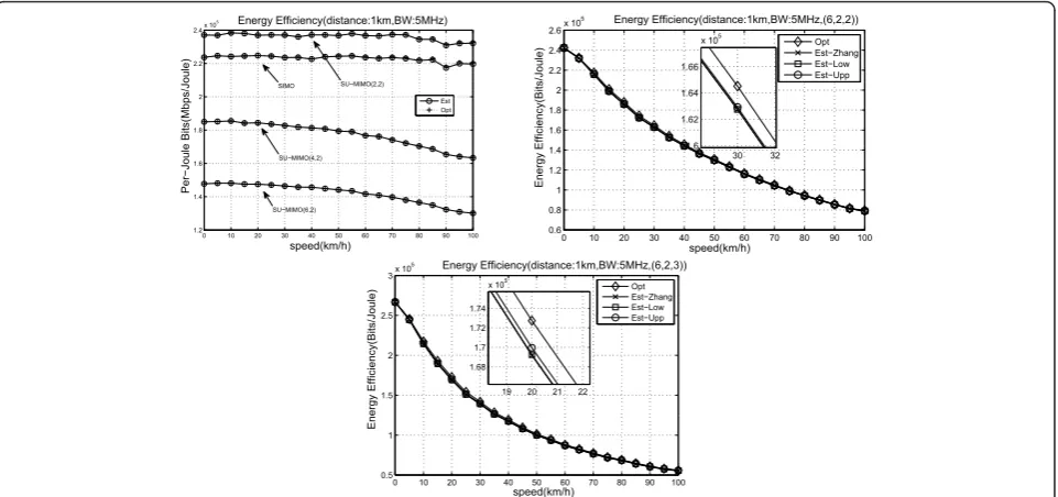
Figure 2 compares the BPJ-EE derived by ergodic capacity estimation schemes and the one by simulations. The left figure demonstrates the SU-MIMO modes. The estimation of SIMO, SU-MIMO (4,2) and SU-MIMO (6,2) is accurate when the moving speed is low. But when the speed is increasing, the ergodic capacity esti-mation of SU-MIMO (4,2) and SU-MIMO (6,2) cannot track the decrease of BPJ-EE. There also exists a gap between the ergodic capacity estimation and the simula-tion in the SIMO mode. Although the mismatching exists, the ergodic capacity-based mode switching can always match the optimal mode, which will be shown in

the next figure. For the MU-MIMO modes, the two lower bound ergodic capacity estimation schemes mis-match the simulation more than the upper bound esti-mation scheme. That is because the lower bound estimations cause BPJ-EE decreasing twice. Firstly, the derived transmit power would mismatch with the exactly accurate transmit power because the derivation is based on a bound and this transmit power mismatch will make the BPJ-EE decrease compared with the simu-lation. Secondly, the lower bound estimation uses a lower bound formula to calculate the estimated BPJ-EE under the derived transmit power, which will make the BPJ-EE decrease again. Nevertheless, the upper bound estimation has the opposite impact on the BPJ-EE esti-mation during the above two steps, so it matches the simulation much better. According to Figures 1 and 2, the upper bound estimation is the best estimation scheme for the MU-MIMO mode. Therefore, during the ergodic capacity-based mode switching, the upper bound estimation is applied.

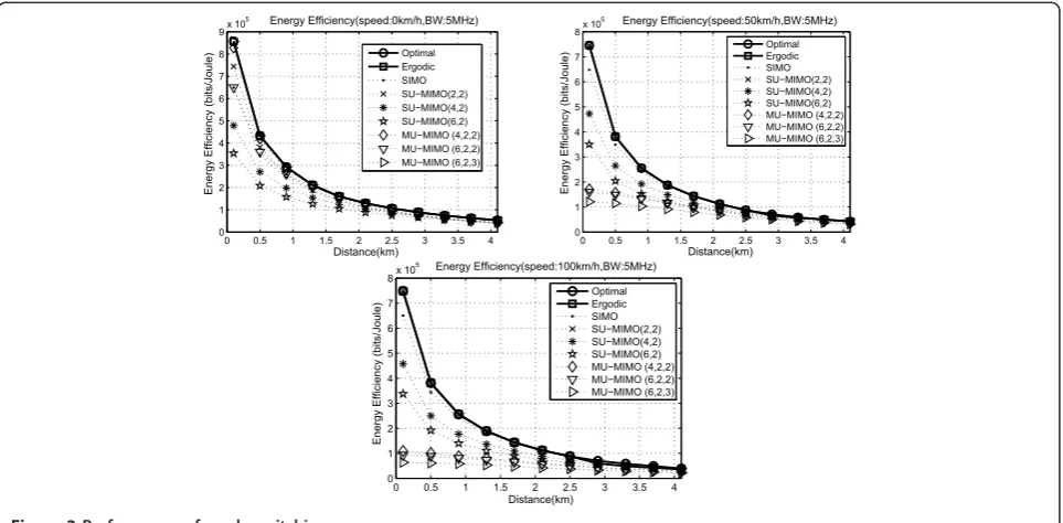
Figure 3 depicts the BPJ-EE performance of mode switching. For comparison, the optimal mode with instant CSIT (’Optimal’) is also plotted. The mode switching can improve the energy efficiency significantly and the ergodic capacity-based mode switching can always track the optimal mode. The performance of ergodic capacity-based switching is nearly the same as the optimal one. Through the simulation, the ergodic capacity-based mode switching is a promising way to choose the most energy-efficient transmission mode.

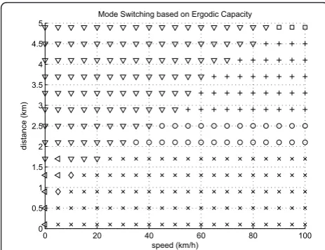
Figure 4 demonstrates the preferred transmission mode under the given scenarios. The optimal mode

Energy Efficiency(distance:1km,BW:5MHz)

Energy Efficiency(Bits/Joule)

speed(km/h)

speed(km/h) speed(km/h)

Energy Efficiency(Bits/Joule)

Per

í

Joule Bits(Mbps/Joule)

Energy Efficiency(distance:1km,BW:5MHz,(6,2,3))

Energy Efficiency(distance:1km,BW:5MHz,(6,2,2))

0 10 20 30 40 50 60 70 80 90 100 1.2

1.4 1.6 1.8 2 2.2 2.4x 10

5

Est Opt SIMO SUíMIMO(2,2)

SUíMIMO(4,2)

SUíMIMO(6,2)

0 10 20 30 40 50 60 70 80 90 100 0.6

0.8 1 1.2 1.4 1.6 1.8 2 2.2 2.4 2.6x 10

5

30 32 1.6

1.62 1.64 1.66

x 105

Opt EstíZhang EstíLow EstíUpp

0 10 20 30 40 50 60 70 80 90 100 0.5

1 1.5 2 2.5

3x 10

5

19 20 21 22 1.68

1.7 1.72 1.74

x 105

Opt EstíZhang EstíLow EstíUpp

under different moving speed and distance is depicted. This figure provides insights into the PC power/dynamic power/static power trade-off and the multiplexing gain/ inter-user interference compromise. When the moving speed is low, MU-MIMO modes are preferred and vice versa. This result is similar to the spectral efficient mode switching in [15-18]. Inter-user interference is small when the moving speed is low, so there is higher multiplexing gain of MU-MIMO benefits. When the moving speed is high, the inter-user interference with

MU-MIMO becomes significant, so SU-MIMO which can totally avoid the interference is preferred. Let us focus on the effect of distance on the mode under high moving speed case then. When distance is less than 1.7 km, SU-MIMO (2,2) is the optimal one, while the dis-tance is equal to 2.1 and 2.5 km, the SIMO mode is sug-gested. When the distance is larger than 2.5 km, the active transmit antenna number increases as the dis-tance increases. The reason of the preferred mode varia-tion can be explained as follows. The total power can be

speed(km/h)

Figure 2Comparison of energy efficiency based on ergodic capacity and instant capacity with SU-MIMO and MU-MIMO.

Energy Efficiency (bits/Joule) Energy Efficiency (bits/Joule)

Distance(km)

divided into PC power, transmit antenna number related power“Dyn-I”and“Dyn-III”and transmit antenna num-ber independent power“Dyn-II”and static power. The first and third part divided by capacity would increase as the active number increases, while the second part is opposite. In the long distance scenario, the first part will dominate the total power and then a more active antenna number is preferred. In the short and medium distance scenario, the second and third part dominate the total power and the trade-off between the two parts should be met. Above all, the above mode switching trends of Fig-ure 4 externalize the two trade-offs.

7. Conclusion

This article discusses the energy efficiency maximizing problem in the downlink MIMO systems. The optimal bandwidth and transmit power are derived for each dedicated mode with constant system parameters, i.e., fixed transmission scheme, fixed active transmit/receive antenna number and fixed active user number. During the derivation, the capacity estimation mechanism is presented and several accurate capacity estimation stra-tegies are proposed to predict the capacity with imper-fect CSIT. Based on the optimal derivation, ergodic capacity-based mode switching is proposed to choose the most energy-efficient system parameters. This method is promising according to the simulation results and provides guidance on the preferred mode over given scenarios.

Appendix A

Proof of Lemma 1

Proof: The proof of the above lemma is motivated by [4]. Denote the inverse function ofy =f(x) asx =g(y),

then x∗ = arg maxx_axf(x₊)_b= arg maxg(y)_ag(yy_)+b. Denotey* =

f(x*). Since f(x) is monotonically increasing,

y∗= arg maxy_ag(y_y)+b. According to [4], there exists a

unique globally optimaly* given by

y∗ = b_ag+ag((yy∗)∗) (36)

ifg(y) is strictly convex and monotonically increasing. (36) is fulfilled since the inverse function ofg(y), i.e.,f(x) is strictly concave and monotonically increasing. Taking

g(y) = 1

f(x) and f(x) =y into (36), we can get (15).

Appendix B

Proof of Theorem 1

Proof:The first part can be proved according to Lemma 1. Calculating the first and second derivation of R(W) based on (8), (10) and (11), we can see that R(W) of both SVD and BD mode is strictly concave and monoto-nically increasing as a function of W. The optimalW* can be got through (15), which is given by (16).

Look at the second part. Taking Pt =ptWinto (8),

(10) and (11), the capacity is R(Pt, W) =WRˆm(pt), where Rˆ(pt) is independent ofW. We have that

ξ = WRˆ(pt)

(Mapsp,bw+pac,bw)W+MaPcir+PPC+PSta. (37)

The second part is verified.

Appendix C

Proof of Theorem 2

Proof:According to Lemma 1, the above theorem can be verified if we prove that Rm(Pt) is strictly concave

and monotonically increasing for both SVD and BD. It is obvious that the capacity of SVD and BD with perfect CSIT is strictly concave and monotonically increasing based on (8) and (10). If the capacity of BD with imper-fect CSIT can also be proved to be strictly concave and monotonically increasing, Theorem 2 can be proved.

Denoting Ak=Ek[n]i=kT (D) i [n]T

(D)H i [n]

EH_k[n],

then rewrite (11) as follows:

RD b(Pt) =W

Ka

k=1

log det(Rk[n] +NPtsHˆeff,k[n]Hˆ H

eff,k[n])−log detRk[n] !

=W

Ka

k=1

log detI+ Pt

N0WNs(Ak+Hˆeff,k[n]Hˆ H eff,k[n])

−log detI+ Pt N0WNsAk

!

=W

Ka

k=1 Na,k

i=1

log1 + Pt N0WNsck,i

−log1 + Pt N0WNsgk,i

!

.

(38)

ck,iandgk,iare the eigenvalue of Ak+Hˆeff,k[n]Hˆ H eff,k[n] and Ak, respectively. Sorting ck,i and gk,i as

ck,1≥ . . . ≥ck,Na,k and gk,1≥ . . . ≥gk,Na,k. Since Ak

0 20 40 60 80 100

0 0.5 1 1.5 2 2.5 3 3.5 4 4.5 5

speed (km/h)

distance (km)

Mode Switching based on Ergodic Capacity

and Heff,ˆ k[n]Hˆ H

eff,k[n] are both positive definite,ck,i> gk,i, i= 1,...,Na,k. Calculating the first and second derivation of (38), (11) is strictly concave and monotonically increasing. Then Theorem 2 is verified.

Acknowledgements

This work is supported in part by Huawei Technologies Co. Ltd., Shanghai, China, Chinese Important National Science and Technology Specific Project (2010ZX03002-003) and National Basic Research Program of China (973 Program) 2007CB310602. The authors would like to thank the anonymous reviewers for their insightful comments and suggestions.

Endnotes

a_{Here, more receive antenna at MS will cause higher MS power}

consumption. However, note that the power consumption of MS is omitted.

Author details

1_{Personal Communication Network & Spread Spectrum Laboratory (PCN&SS),}

University of Science and Technology of China (USTC), Hefei, 230027 Anhui, China2_{Wireless research, Huawei Technologies Co. Ltd., Shanghai, China}

Competing interests

The authors declare that they have no competing interests.

Received: 22 February 2011 Accepted: 9 December 2011 Published: 9 December 2011

References

1. G Fettweis, Ernesto Zimmermann, ICT Energy Consumption - Trends And Challenges. proc of WPMC. (2008)

2. O Blume, D Zeller, U Barth, Approaches to Energy Efficient Wireless Access Networks. Proceedings of the 4th International Symposium on

Communications. Control and Signal Processing, ISCCSP 2010, Limassol, Cyprus. 3–5 (2010)

3. H Kim, G de Veciana, Leveraging Dynamic Spare Capacity in Wireless System to Conserve Mobile Terminals’Energy. IEEE/ACM Trans Netw.

18(3):802–815 (2010)

4. GW Miao, N Himayat, GY Li, D Bormann, Energy-efficient design in wireless OFDMA. Proc IEEE 2008 International Conference on Communications, Beijing, China. 3307_–3312 (2008)

5. GW Miao, N Himayat, GY Li, A Swami, Cross-layer optimization for energy-efficient wireless communications: a survey, (invited). Wiley J Wirel Commun Mobile Comput.9(4):529–542 (2009). doi:10.1002/wcm.698 6. GW Miao, N Himayat, GY Li, Energy-efficient link adaptation in

frequency-selective channels. IEEE Trans Commun.58(2):545–554 (2010) 7. S Zhang, Y Chen, S Xu, Improving Energy Efficiency through Bandwidth,

Power, and Adaptive Modulation. IEEE Proceeding of 2010 Vehicular Technology Conference Fall

8. S Cui, AJ Goldsmith, A Bahai, Energy-efficiency of MIMO and cooperative MIMO techniques in sensor networks. IEEE J Sel Areas Commun.

22(6):1089_–1098 (2004). doi:10.1109/JSAC.2004.830916

9. H Kim, C-B Chae, G Veciana, RW Heath, A cross-layer approach to energy efficiency for adaptive MIMO systems exploiting spare capacity. IEEE Trans Wirel Commun.8(8) (2009)

10. HS Kim, B Daneshrad, Energy-constrained link adaptation for MIMO OFDM wireless communication systems. IEEE Trans Wirel Commun.9(9):2820–2832 (2010)

11. QH Spencer, AL Swindlehurst, M Haardt, Zero-forcing methods for downlink spatial multiplexing in multi-user MIMO channels. IEEE Trans Signal Process.

52(2):461_–471 (2004). doi:10.1109/TSP.2003.821107

12. Z Shen, R Chen, JG Andrews, RW Heath Jr, BL Evans, Low complexity user selection algorithms for multiuser MIMO systems with block diagonalization. IEEE Trans Signal Process.54(9):3658–3663 (2006)

13. Z Shen, R Chen, JG Andrews, RW Heath Jr, BL Evans, Sum capacity of multiuser MIMO broadcast channels with block diagonalization. IEEE Trans Wirel Commun.6(6):2040–2045 (2007)

14. R Chen, Z Shen, JG Andrews, RW Heath Jr, Multimode transmission for multiuser MIMO systems with block diagonalization. IEEE Trans Signal Process.56(7):3294–3302 (2008)

15. J Zhang, RW Heath Jr, M Kountouris, JG Andrews, Mode switching for the multi-antenna broadcast channel based on delay and channel quantization. EURASIP J Adv Signal Process15(2009). Article ID 802548

16. J Zhang, JG Andrews, RW Heath Jr, Block Diagonalization in the MIMO Broadcast Channel with Delayed CSIT. IEEE proc of Globecom. 1_–6 (2009) 17. J Zhang, M Kountouris, JG Andrews, RW Heath Jr, Multi-mode transmission

for the MIMO broadcast channel with imperfect channel state information. IEEE Trans Commun.59(3):803–814 (2011)

18. J Xu, L Qiu, Robust Multimode Selection in the Downlink Multiuser MIMO Channels with Delayed CSIT. IEEE proc of ICC. 1–5 (2011)

19. O Arnold, F Richter, G Fettweis, O Blume, Power Consumption Modeling of Different Base Station Types in Heterogeneous Cellular Networks. Proceedings of the ICT MobileSummit (ICT Summit’10), Florence, Italy. 16_–18 (2010)

20. IE Telatar, Capacity of multi-antenna Gaussian channels. Europ Trans Telecommun.10, 585_–595 (1999). doi:10.1002/ett.4460100604 21. J Xu, L Qiu, C Yu, Link Adaptation and Mode Switching for the Energy

Efficient Multiuser MIMO Systems, submitted to IEICE Trans. Commun Available online at http://home.ustc.edu.cn/~suming/

22. T Yoo, AJ Goldsmith, Capacity and power allocation for fading MIMO channels with channel estimation error. IEEE Trans Inf Theory.

52(5):2203–2214 (2006)

23. P Rapajic, D Popescu, Information capacity of a random signature multiple-input multiple-output channel. IEEE Trans Commun.48, 1245–1248 (2000). doi:10.1109/26.864159

doi:10.1186/1687-1499-2011-200

Cite this article as:Xuet al.:Improving energy efficiency through multimode transmission in the downlink MIMO systems.EURASIP Journal on Wireless Communications and Networking20112011:200.

Submit your manuscript to a

journal and benefi t from:

7Convenient online submission

7Rigorous peer review

7Immediate publication on acceptance

7Open access: articles freely available online

7High visibility within the fi eld

7Retaining the copyright to your article