R E S E A R C H
Open Access
A new compact high order off-step
discretization for the system of 2D
quasi-linear elliptic partial differential
equations
Ranjan K Mohanty
1*and Nikita Setia
2*Correspondence: [email protected];
[email protected] 1Department of Applied Mathematics, Faculty of Mathematics and Computer Science, South Asian University, Akbar Bhawan, Chanakyapuri, New Delhi, 110021, India
Full list of author information is available at the end of the article
Abstract
A new fourth-order difference method for solving the system of two-dimensional quasi-linear elliptic equations is proposed. The difference scheme referred to as off-step discretizationis applicable directly to the singular problems and problems in polar coordinates. Also, new fourth-order methods for obtaining the first-order normal derivatives of the solution are developed. The convergence analysis of the proposed method is discussed in details. The methods are applied to many physical problems to illustrate their accuracy and efficiency.
MSC: 65N06
Keywords: quasi-linear elliptic equations; fourth-order finite difference methods; convection-diffusion equation; Burger’s equation; Poisson’s equation in polar coordinates; Navier-Stokes equations of motion
1 Introduction
We consider the two-dimensional (D) quasi-linear elliptic partial differential equation (PDE) of the type
a(x,y,u)uxx+b(x,y,u)uyy=f(x,y,u,ux,uy), ()
where (x,y)∈R= (, )×(, ), with boundary∂R(see Figure ), subject to the Dirichlet boundary conditions given by
u(x,y) =v(x,y), (x,y)∈∂R. ()
The PDEs of the type () with variable coefficients model many problems of physical sig-nificance. For instance, the convection-diffusion and Burgers’ equations that represent the transport phenomena, and the highly nonlinear Navier-Stokes’ (N-S) equations of motion that describe the motion of fluid flow and represent the conservation of mass, momentum and energy.
We make the following assumptions about the boundary value problem ():
(a) ab> inR,
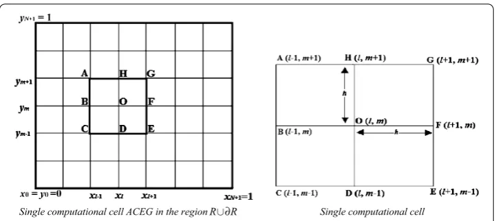
Figure 1 Schematic representation of two dimensional nine point compact cell.
(b) u(x,y)∈C,
(c) a,b∈C,
(d) f is continuous, (e) ∂∂fu≥,
(f ) |∂∂ufx| ≤H, (g) |∂∂uf
y| ≤I,
whereH andI are positive constants andCm is the set of all functions ofxandywith continuous partial derivatives up to ordermin the regionR. The condition (a) guarantees the ellipticity of equation (). Conditions (e), (f ) and (g) are the necessary conditions for the existence and uniqueness of the solution of boundary value problem ()-() (see []).
A number of high order compact schemes have been reported for the linear ellip-tic problems like Poisson’s equation and the convection diffusion equation (see [–]). Ananthakrishnaiah and Saldanha [] framed a -point fourth-order compact scheme for the solution of a scalar nonlinear elliptic PDE, which was later extended to a system of equations by Saldanha []. The finite difference methods for solving the steady state incompressible N-S equations vary considerably in terms of accuracy and efficiency. It has been discovered that although central difference approximations are locally second-order accurate, they often suffer from computational instability and the resulting solutions ex-hibit non-physical oscillations. The upwind difference approximations, though computa-tionally stable, are only first-order accurate and the resulting solutions exhibit the effects of artificial viscosity. A number of high order compact schemes for the solution of the N-S equations in stream function vorticity form in the Cartesian coordinates were pro-posed in [–]. In , Mohanty [] propro-posed fourth-order difference methods for D nonlinear elliptic boundary value problems with variable coefficients using only nine grid points of a single computational cell. This method could be successfully applied to the N-S model equations in polar coordinates. Later, Mohanty and Dey [] developed the fourth-order accurate estimates of the first-order normal derivatives of the solution
In this article, we develop new off-step fourth-order discretizations for the solution of the system of quasi-linear elliptic PDEs with variable coefficients, and the estimates of (∂u/∂n), using the nine grid points of a single computational cell (see Figure ). The main advantage of the proposed methods is that they are directly applicable to the singular prob-lems and the probprob-lems in polar coordinates, without any need of modifications, hence reducing the manual and mechanical calculations reasonably.
An outline of the article is as follows: In Section , we discuss and derive the off-step fourth-order compact discretization schemes for the solution of a nonlinear elliptic equa-tion with variable coefficients and the estimates of (∂u/∂n). These methods are further extended to the solution of the quasi-linear PDE given by ()-(). In Section , we estab-lish the fourth-order convergence of the method for a scalar equation under appropriate conditions. Further, in Section , the stability analysis of the steady state convection dif-fusion equation is conducted. In Section , we generalize our methods for the system of quasi-linear PDEs with variable coefficients, subject to the Dirichlet boundary conditions. In Section , we implement the proposed methods over linear and nonlinear problems of physical significance to illustrate and examine the accuracy of these methods. Section contains some concluding remarks about this article.
2 The off-step discretization and derivation
We first consider the following two-dimensional nonlinear elliptic PDE:
a(x,y)uxx+b(x,y)uyy=f(x,y,u,ux,uy) ()
for (x,y)∈R, subject to the Dirichlet boundary conditions given by ().
We superimpose on the domainRa rectangular grid with spacingh> in bothxand
y-directions. Let us introduce the following notations:
(a) Each grid point is given by(xl,ym)or simply(l,m)forxl=lhandym=mh, ≤l,m≤N+ , where(N+ )h= .
Further, at each grid point (l,m), let:
(b) Ul,mandul,mdenote the exact and approximate values ofu(xl,ym), respectively.
(c) fl,m=f(xl,ym,Ul,m,Uxl,m,Uyl,m).
(d) ForS=a,b,U,α,βandγ, let
Spq=
∂p+qS
∂xp∂yq, p,q= , , , . . . .
Then, for ≤l,m≤N+ , differential equation () can be written as
aU+bU=fl,m. ()
For the fourth-order discretization of PDE (), we simply follow the approach given by Chawla and Shivakumar [].
We set the following approximations:
Ul±
,m= (Ul±,m+Ul,m)/, (.)
Ul,m±
Uxl,m= (Ul+,m–Ul–,m)/(h), (.)
Uxl±
,m= (±Ul±,m∓Ul,m)/(h), (.) Uxl,m±
= (Ul+,m±–Ul–,m±+Ul+,m–Ul–,m)/(h), (.)
Uyl,m= (Ul,m+–Ul,m–)/(h), (.)
Uyl±
,m= (Ul±,m+–Ul±,m–+Ul,m+–Ul,m–)/(h), (.)
Uyl,m±
= (±Ul,m±∓Ul,m)/(h), (.)
Uxxl,m= (Ul+,m– Ul,m+Ul–,m)/
h, (.)
Uxxl,m±= (Ul+,m±– Ul,m±+Ul–,m±)/
h, (.)
Uyyl,m= (Ul,m+– Ul,m+Ul,m–)/
h, (.)
Uyyl±,m= (Ul±,m+– Ul±,m+Ul±,m–)/
h. (.)
Define
fl±
,m=f(xl±,ym,Ul±,m,Uxl±,m,Uyl±,m), (.)
fl,m±
=f(xl,ym±,Ul,m±,Uxl,m±,Uyl,m±). (.)
Let
Ul,m=Ul,m+ph(fl+
,m+fl–,m) +ph
(f
l,m+ +fl,m–)
+phUxxl,m+phUyyl,m, (.)
Uxl,m=Uxl,m+qh(fl+,m–fl–,m) +qh(Uyyl+,m–Uyyl–,m)
+qhUxxl,m+qhUyyl,m, (.)
Uyl,m=Uyl,m+rh(fl,m+ –fl,m–) +rh(Uxxl,m+–Uxxl,m–)
+rhUxxl,m+rhUyyl,m, (.)
wherepks,qks andrks (≤k≤) are the parameters to be suitably determined. Finally, define
fl,m=f(xl,ym,Ul,m,Uxl,m,Uyl,m). ()
Then, at each internal grid point (l,m), differential equation () is discretized by
L[U]≡Iδx+Iδy+I
δxμyδy
+I
δyμxδx
+I
δxδyUl,m
=h[Jfl+,m+Jfl–,m+Jfl,m+ +Jfl,m–– fl,m]
forTl,m=O(h), where we denote ference operators inx-directionetc.
Now, with the help of Taylor series expansion, it is easy to obtain
L[U] =h[Jfl+,m+Jfl–,m+Jfl,m+ +Jfl,m– – fl,m] +O
Using (.) and (.) and simplifying (.)-(.) by Taylor series expansions, we obtain
fl±
Using equations (.), (.), simplifying (.)-(.) and (.)-(.), we obtain
Finally, from (), using (.)-(.), we obtain
fl,m=fl,m+
h
T+O
h, ()
where
T=Tα+Tβ+Tγ.
Substituting approximations (.), (.) and () into (), and by the help of (), we ob-tain
Tl,m=
h
(T–T–T) +O
h. ()
Thus, for the proposed difference method () to be of fourth order, the coefficient ofhin () must be zero, and hence we have
T+T– T= .
Equating to zero the coefficients of each ofα,βandγ, we obtain the values of the unknown parameters as follows:
p= /(a), p= /(b), p= ( –a/b)/, p= ( –b/a)/,
q= /(a), q= ( –b/a)/, q= –a/(a), q= –b/(a),
r= /(b), r= ( –a/b)/, r= –a/(b), r= –b/(b)
thereby reducingTl,mtoO(h). Thus the difference method ofO(h) for nonlinear PDE () is given by () for the above values of parameters.
Now, we consider the numerical method ofO(h) for the solution of D quasi-linear elliptic equation (). In order to understand the concept to develop the method for the quasi-linear case, we consider the following differential equation:
u=f(x), <x< . ()
A fourth-order method for differential equation () is given by
Ul–– Ul+Ul+=
h
fl+hfxxl
+Oh, ()
whereUl=u(xl),fl=f(xl) andfxxl=∂
f
l
∂x.
Whenever the differential equation () is of the formu=f(x,u), the evaluation offxxis difficult and formula () needs to be modified. Substitutinghf
xxl=fl+– fl+fl–+O(h) in (), we obtain the modified version of () due to Numerov as
Ul–– Ul+Ul+=
h
[fl++fl–+ fl] +O
h, ()
Now, we use the above concept to derive the numerical method for quasi-linear equation (). Since the coefficients are the functions of not only the independent variablesxand
ybut also of the dependent variableu,i.e.,a=a(x,y,u) andb=b(x,y,u), the difference scheme () cannot be applied directly as the first- and second-order derivatives ofuare unknown at the internal grid points. Thus further discretizations ofux,uy,uxxanduyyare required in the method () without affecting its order. For this purpose, forS=aandb, we use the following central differences:
S= (Sl+,m–Sl–,m)/h+O
h, (.)
S= (Sl,m+–Sl,m–)/h+O
h, (.)
S= (Sl+,m– S+Sl–,m)/h+O
h, (.)
S= (Sl,m+– S+Sl,m–)/h+O
h, (.)
where
S=S(xl,ym,Ul,m),
Sl±,m=S(xl±,ym,Ul±,m),
Sl,m±=S(xl,ym±,Ul,m±).
Upon substitution of the central differences (.)-(.) in the method (), it is easy to verify that
I= a+
[al+,m+al–,m+al,m++al,m–]
–(al,m+–al,m–)(bl,m+–bl,m–) b
–(al+,m–al–,m)
a
+Oh,
I= b+
[bl+,m+bl–,m+bl,m++bl,m–]
–(al+,m–al–,m)(bl+,m–bl–,m) a
–(bl,m+–bl,m–)
b
+Oh,
I=
(al,m+–al,m–)
–
bl,m+–bl,m– b
a+O
h,
I=
(bl+,m–bl–,m)
–
al+,m–al–,m a
b+O
h.
We observe that the truncation errorTl,mretains its orderO(h), and hence we obtain the required numerical method ofO(h) for the solution of quasi-linear elliptic PDE ().
After having determined the fourth-order approximations to the solution of equation (), we now discuss the fourth-order numerical methods for the estimates of (∂u/∂x) and (∂u/∂y). One may compute these values using the standard central differences:
uxl,m= (ul+,m–ul–,m)/(h), (.)
It is found that the standard central differences (.) and (.) yield second-order ac-curate results irrespective of whether fourth-order difference method () or standard dif-ference scheme is used to solve PDE (). Thus, new difference methods for computing the numerical values of (∂u/∂x) and (∂u/∂y) are developed, which are found to yieldO(h) accurate results when used in conjunction with the nine-point formula ().
At each grid point (l,m), we denote the exact and the approximate solutions of (∂u/∂x),
A simple Taylor series expansion would yield
Uxl,m= first-order normal derivatives of the solution of nonlinear equation (). The numerical methods (.)-(.) are applicable when the fourth-order numerical solutions ofuare known at each internal grid point. Further, the Dirichlet boundary conditions are given by (). The difference method () for the determination ofucan be easily expressed in tri-block-diagonal matrix form, and the methods (.)-(.) for determination of (∂u/∂x) and (∂u/∂y) can be expressed in diagonal matrices form, thus can be easily solved. The proposed methods (), (.) and (.) are directly applicable to singular elliptic problems in the regionR.
3 Convergence analysis
We consider the D nonlinear elliptic partial differential equation
Auxx+Buyy=f(x,y,u,ux,uy) ()
defined in the regionR, subject tou(x,y) =v(x,y), (x,y)∈∂R, whereA,B> are constants. Then the difference method () for equation () is given by
Aδx+ Bδy+(A+B) δ
xδy ul,m
= h[fl+
,m+fl–,m+fl,m+ +fl,m––fl,m]; ≤l,m≤N. ()
Let, for each (l,m) such that ≤l,m≤N,
Ml,m= h[fl+,m+fl–,m+fl,m++fl,m– –fl,m] + boundary values
andEl,m=ul,m–Ul,m.
Also, forS=M,u,U,T andE, let
S= [S,,S,, . . . ,SN,,S,,S,, . . . ,SN,, . . . ,S,N,S,N, . . . ,SN,N]tN×,
where t denotes the transpose of the matrix.
Then, varying (l,m) such that ≤l,m≤N, equation () may be written in the matrix form as
Du+M(u) =, ()
where
D=
K R K
N×N (Tri-block diagonal matrix)
for
R=–A+B (A+B) –A+B
N×N (Tri-diagonal matrix)
and
K=
–(A+B)/ –B+A –(A+B)/
N×N (Tri-diagonal matrix).
We assume here thatB< AandA< B. Thus, all the diagonal entries of matrixDare positive and all the off-diagonal entries are negative.
SinceUis the exact solution vector, we have
DU+M(U) +T=, ()
Now, let
With the help of equations (.)-(.) and (.)-(.), we obtain
P(m–)N+l,mN+l±=
h
±Hl(),m+Il(),m+h
±Hyl(),m±Ixl(),m∓Il(),mHl(),m∓Hl(),mI()l,m
+Oh [≤l≤N– , ≤l≤N, ≤m≤N– ],
P(m–)N+l,(m–)N+l±=
h
±Hl(),m–I()l,m+h
∓Hyl(),m∓Ixl(),m±Il(),mHl(),m±Hl(),mIl(),m
+Oh [≤l≤N– , ≤l≤N, ≤m≤N].
Using relation (), from equations () and (), in the absence of round-off errors, we obtain the error equation
(D+P)E=T. ()
LetR=R∪∂Rand
G∗= min
(x,y)∈R
∂f
∂U and G
∗= max
(x,y)∈R
∂f ∂U,
then
<G∗≤G()l± ,m
,G()
l,m±,G () l,m≤G∗
and forQ=HandI, let
<Q()
l±,m,Q () l,m±,Q
() l,m≤Q
and
Q()
xl,m≤Q(), Q ()
yl,m≤Q()
for some positive constantsQ,Q()andQ().
Now, it is easy to verify that for sufficiently smallh,
|P(m–)N+l,(m–)N+l|< [≤l≤N, ≤m≤N],
|P(m–)N+l,(m–)N+l±|< [≤l≤N– , ≤l≤N, ≤m≤N], |P(m–)N+l,(m–±)N+l|< [≤l≤N, ≤m≤N– , ≤m≤N], |P(m–)N+l,mN+l±|< [≤l≤N– , ≤l≤N, ≤m≤N– ], |P(m–)N+l,(m–)N+l±|< [≤l≤N– , ≤l≤N, ≤m≤N].
For ≤r≤N– ,
S(k–)N+r= B+h
G()r,k+ G()r,k– G()r,k+h
[b(k–)N+r+hc(k–)N+r] +O
h,
where
b(k–)N+r=±Ir(),k±I () r,k∓I
() r,k,
c(k–)N+r= –Iyr(),k+I () r,kI
() r,k.
(.)
And finally, forq= ()N– ,r= ()N– ,
S(r–)N+q=h
Gq(),r+ Gq(),r– G()q,r
+Oh. (.)
With the help of equations (.)-(.), we get
|bk| ≤(H+I), |ck| ≤
H+I+ H()+I()+ H()+I()+ IH
fork= ,N, (N– )N+ andN,
|bk| ≤H, |ck| ≤H()+H
fork= (q– )N+ andqN; ≤q≤N– ,
|bk| ≤I, |ck| ≤I()+I
fork=rand (N– )N+r; ≤r≤N– .
It follows that for sufficiently smallh,
Sk> hG∗
fork= ,N, (N– )N+ andN, (.)
Sk> hG∗
fork= (q– )N+ andqN; ≤q≤N– , (.)
Sk> hG∗
fork=rand (N– )N+r; ≤r≤N– , (.)
S(r–)(N–)+q≥h
G∗– G∗> , assumingG∗< G∗
for ≤q≤N– and ≤r≤N– . (.)
Thus, for sufficiently smallh,D+Pis monotone. Hence (D+P)–exists and (D+P)–= J–>(see Henrici []), where
J= (Jr,s)
Since
Equation () may be written as
E ≤ JT, ()
Using equations (.)-(.) in equation (), from () we obtain, for sufficiently smallh,
E ≤Oh. ()
This establishes the convergence of the fourth-order difference method () (withn= ) for the scalar elliptic equation ().
4 Stability analysis
We consider the steady state two-dimensional convection-diffusion equation
whereβ= (/ε) > is a constant, withε(the perturbation parameter) being the ratio of convective velocity to the diffusion coefficient.
Applying the difference scheme () withTl,m= to the above equation and lettingτ= (βh/) > , which is called thecell Reynolds number, we obtain
+ τul,m
= ( +τ)ul–,m–+ ul,m–+ ( –τ)ul+,m–+
–τ+τul–,m
+ – +τ+τul+,m+ ( +τ)ul–,m++ ul,m++ ( –τ)ul+,m+. ()
The above is a system ofN number of linear equations inNnumber of unknowns, which may be expressed in the matrix form asAu=B, where
A=P Q P
N×N (Tri-block-diagonal matrix),
P= +τ –τ
N×N (Tri-diagonal matrix),
Q=
( –τ+τ) –( + τ) (– +τ+τ)
N×N (Tri-diagonal matrix),
B:N× matrix consisting of boundary values.
Now, applying the Jacobi iteration method to the above system of equations, we obtain
+ τu(l,sm+)
= ( +τ)u(ls–,) m–+ u(l,sm)–+ ( –τ)u(l+,s) m–+ –τ+τu(l–,s) m
+ – +τ+τul(+,s) m+ ( +τ)u(ls–,) m++ u(l,sm)++ ( –τ)u(ls+,) m+, ()
wheres= , , , . . . .
We examine the stability of () by assuming that an errorεl(s,m) exists at each grid point (l,m) at thesth iteration. We analyze the behavior of the errorεl(,sm) by assuming it to be of the form
ε(l,sm) =ξsAlBmsin
πal N
sin
πbm
N
, ≤a,b≤N, ()
whereAandBare arbitrary constants andξis the propagating factor which determines the rate of growth or decay of the errors. The necessary and sufficient condition for the iterative method to be stable is|ξ|< .
Using () in (), the propagating factor for the Jacobi iteration method is obtained as
ξJ=
[( –τ)cos(πb
N) – +τ+τ
]/[( +τ)cos(πb
N) + –τ+τ
]/cos(πa
N ) + cos(
πb N)
+τ ,
≤a,b≤N. ()
propa-gation factorξGSis given by the equation
η–
ψ+φ –τ+τ( –τ)cos
πb
N η
+
ψ– –τ+τ– +τ+τφ– –τcos
πb N
φ η
– φ( +τ)– +τ+τcos
πb N
= , ≤a,b≤N, ()
whereη=ξGS/,φ=cos(πNa)
+τ andψ=
cos(πNb) +τ.
Thus, the Gauss-Siedal iteration method is stable for those values ofτsuch that|ξGS|< .
5 Generalisation of the above methods
We now extend our methods to the system of D quasi-linear elliptic PDEs of the form:
a(i)u(xxi)+b(i)uyy(i)=f(i), ≤i≤n ()
for (x,y)∈R, with eacha(i)=a(i)(x,y,u(),u(), . . . ,u(n)),b(i)=b(i)(x,y,u(),u(), . . . ,u(n)) and
f(i) =f(i)(x,y,u(),u(), . . . ,u(n),u()x ,u()x , . . . ,u(xn),u()y ,u()y , . . . ,u(yn)), subject to the Dirichlet boundary conditions given by
u(i)(x,y) =v(i)(x,y). ()
We assumeUl(,im) andul(,im) to be the exact and approximate values of u(i)(x
l,ym) respec-tively. For each i= ()n, lettingfl(,mi) =f(i)(x
l,ym,Ul(),m,Ul(),m, . . . ,Ul(,nm),Uxl(),m,Uxl(),m, . . . ,Uxl(n,)m,
Uyl(),m,Uyl(),m, . . . ,Uyl(n,)m), we set the following approximations:
U(l±i) ,m=
Ul(±i),m+Ul(,im)/, (.)
U(l,im)± =
Ul(,im)±+Ul(,im)/, (.)
Uxl(i),m=Ul(+,i)m–Ul(–,i) m/(h), (.)
U(xli)± ,m=
±Ul(±i),m∓Ul(,im)/(h), (.)
U(xli),m± =
Ul(+,i)m±–Ul(–,i) m±+Ul(+,i) m–Ul(–,i)m/(h), (.)
Uyl(i),m=Ul(,im)+–Ul(,im)–/(h), (.)
U(yli)± ,m=
Ul(±i),m+–Ul(±i),m–+Ul(,im)+–Ul(,im)–/(h), (.)
U(yli),m± =
±Ul(,im)±∓Ul(,im)/(h), (.)
Uxxl(i),m=Ul(+,i)m– Ul(,im) +Ul(–,i) m/h, (.)
Uxxl(i),m±=Ul(+,i) m±– Ul(,im)±+Ul(–,i)m±/h, (.)
Uyyl(i),m=Ul(,im)+– Ul(,im) +Ul(,im)–/h, (.)
Define
Then, at each internal grid point (l,m), the fourth-order off-step discretization to each differential equation of system () is given by
forT(l,im) =O(h), where we denote
After the fourth-order approximate solution to system () is determined upon solv-ing the tri-block diagonal system of equations (), it is easy to see that the fourth-order estimates of (∂u(i)/∂n) can be explicitly obtained using the following discretizations:
Uxl(i),m=
solved using the block iterative method and the system of nonlinear difference equations by the Newton-Raphson method (see Hageman and Young [], Kelly [] and Saad []). The iterations are terminated once the absolute error tolerance≤–has been reached. All the computations are done using MATLAB programming language.
Example (Convection-diffusion equation)
uxx+uyy=βux, <x,y< ()
subject to the Dirichlet boundary conditions given by
u(x, ) = ,
u(x, ) = for <x< ,
u(,y) =sinπy,
u(,y) = sinπy for <y< .
The solutionuto the above equation and its first-order derivativesuxanduyat the point (., .) are listed in Table forβ= and . Figure gives the plot of the numerical solution to Example .
Example (Poisson’s equation inr-θplane)
urr+
α rur+
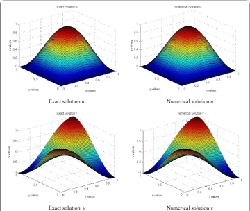
ruθ θ=G(r,θ), <r,θ< . () Atα= and , the above equation represents D Poisson’s equation in cylindrical and spherical coordinates, respectively. The exact solution isu=rcos(π θ).
The maximum absolute errors (MAE) inu,uxanduyare listed in Table forα= and . Figure gives the plots of the exact and numerical solutions to Example .
Example (Poisson’s equation inr-zplane)
urr+
α
rur+uzz=G(r,z), <r,z< . ()
Table 1 Example 1: convection diffusion equation (51) at the point (0.5, 0.5)
h ProposedO(h4)-methods O(h2)-Methods
β= 10 β= 50 β= 10 β= 50
1/8 u 6.4316(–01) 9.0714(–01) 6.4284(–01) Diverges ux –5.0091(–01) –1.8812(–01) –5.1892(–01) Diverges
uy 1.0190(–12) 1.8459(–13) –1.1529(–12) Diverges
1/16 u 6.4286(–01) 9.0637(–01) 6.4275(–01) 9.0666(–01) ux –5.0104(–01) –1.7821(–01) –5.0464(–01) –1.7790(–01)
uy 2.2231(–12) 4.5889(–15) –3.1806(–12) 3.4461(–13)
1/32 u 6.4284(–01) 9.0637(–01) 6.4281(–01) 9.0644(–01) ux –5.0105(–01) –1.7821(–01) –5.0190(–01) –1.7808(–01)
uy 4.4296(–12) 6.8094(–15) –6.4109(–12) 1.7764(–15)
1/64 u 6.4284(–01) 9.0637(–01) 6.4283(–01) 9.0639(–01) ux –5.0105(–01) –1.7821(–01) –5.0126(–01) –1.7818(–01)
Figure 3 Numerical solutions of 2D convection diffusion equation at (0.5, 0.5).
Table 2 Example 2: Poisson’s equations (52) inr-θplane
h ProposedO(h4)-methods O(h4)-Methods discussed in [16, 17]
α= 1 α= 2 α= 1 α= 2
1/8 u 2.3294(–06) 4.6091(–06) 4.2944(–06) 6.8672(–06) ur 8.1179(–06) 1.6529(–05) 8.8246(–06) 4.2834(–05)
uθ 3.9153(–04) 6.2317(–04) 4.4823(–04) 8.6298(–04)
1/16 u 1.4731(–07) 2.9153(–07) 2.7278(–07) 4.4629(–06) ur 9.7119(–07) 1.8818(–06) 8.1105(–07) 3.0421(–06)
uθ 2.8537(–05) 4.5514(–05) 3.2188(–05) 6.3244(–05)
1/32 u 9.2898(–09) 1.8373(–08) 1.8642(–08) 3.2187(–07) ur 7.9264(–08) 1.5078(–07) 7.0243(–08) 2.2424(–07)
uθ 1.9185(–06) 3.0633(–06) 2.3156(–06) 4.4341(–06)
1/64 u 5.8207(–10) 1.1480(–09) 1.1022(–09) 1.9068(–08) ur 5.5941(–09) 1.0553(–08) 5.8124(–09) 1.4172(–08)
uθ 1.2425(–07) 1.9850(–07) 1.5510(–07) 2.7012(–07)
Table 3 Example 3: Poisson’s equations (53) inr-zplane
h ProposedO(h4)-methods O(h4)-Methods discussed in [16, 17]
α= 1 α= 2 α= 1 α= 2
1/8 u 1.6604(–06) 2.8030(–06) 2.8604(–06) 4.2166(–06) ur 1.0721(–05) 1.0390(–05) 2.1444(–05) 1.9833(–05)
uz 2.3486(–05) 3.6014(–05) 3.6218(–05) 4.8412(–05)
1/16 u 1.0530(–07) 1.7649(–07) 1.9884(–07) 2.6261(–07) ur 8.1375(–07) 8.1496(–07) 1.1721(–06) 1.0104(–06)
uz 1.6895(–06) 2.5690(–06) 2.7520(–06) 3.8224(–06)
1/32 u 6.6915(–09) 1.1082(–08) 1.1645(–08) 1.6224(–08) ur 5.6905(–08) 5.8312(–08) 8.2169(–07) 7.6186(–08)
uz 1.1430(–07) 1.7298(–07) 1.6644(–07) 2.3242(–07)
1/64 u 4.2259(–10) 6.9292(–10) 7.0120(–10) 8.8844(–10) ur 4.5970(–09) 7.3664(–09) 5.0210(–08) 4.5458(–09)
uz 7.4703(–09) 1.1278(–08) 8.9744(–09) 1.4242(–08)
Figure 5 Exact and numerical solutions of 2D Poisson’s equation with cylindrical symmetry.
Atα = , the above represents the two-dimensional Poisson’s equation in cylindrical polar coordinates inr-zplane. The exact solution isu=coshrcoshz.
The MAE inu,uxanduyare listed in Table forα= and . Figure gives the plots of the exact and numerical solutions to Example .
Example (Burger’s equation)
ε(uxx+uyy) =u(ux+uy) +g(x,y), <x,y< . ()
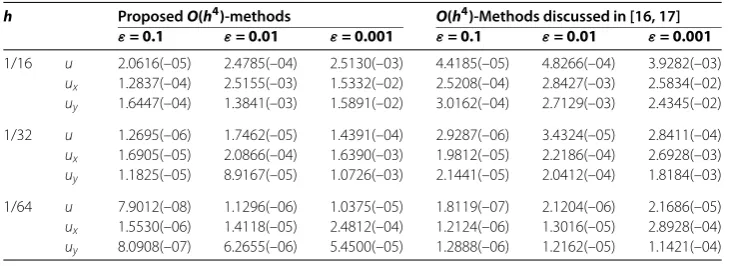
The exact solution isu=exsin(πy). The MAE inu,uxanduyare listed in Table for
ε= ., . and ..
Example (Nonlinear elliptic equation)
+xuxx+
+yuyy=αu(ux+uy) +f(x,y), <x,y< ()
with the exact solutionu=exsin(πy). The MAE foru,u
Table 4 Example 4: Burger’s equation (54)
h ProposedO(h4)-methods O(h4)-Methods discussed in [16, 17] ε= 0.1 ε= 0.01 ε= 0.001 ε= 0.1 ε= 0.01 ε= 0.001
1/16 u 2.0616(–05) 2.4785(–04) 2.5130(–03) 4.4185(–05) 4.8266(–04) 3.9282(–03) ux 1.2837(–04) 2.5155(–03) 1.5332(–02) 2.5208(–04) 2.8427(–03) 2.5834(–02)
uy 1.6447(–04) 1.3841(–03) 1.5891(–02) 3.0162(–04) 2.7129(–03) 2.4345(–02)
1/32 u 1.2695(–06) 1.7462(–05) 1.4391(–04) 2.9287(–06) 3.4324(–05) 2.8411(–04) ux 1.6905(–05) 2.0866(–04) 1.6390(–03) 1.9812(–05) 2.2186(–04) 2.6928(–03)
uy 1.1825(–05) 8.9167(–05) 1.0726(–03) 2.1441(–05) 2.0412(–04) 1.8184(–03)
1/64 u 7.9012(–08) 1.1296(–06) 1.0375(–05) 1.8119(–07) 2.1204(–06) 2.1686(–05) ux 1.5530(–06) 1.4118(–05) 2.4812(–04) 1.2124(–06) 1.3016(–05) 2.8928(–04)
uy 8.0908(–07) 6.2655(–06) 5.4500(–05) 1.2888(–06) 1.2162(–05) 1.1421(–04)
Table 5 Example 5: nonlinear equation (55)
h ProposedO(h4)-methods O(h4)-Methods discussed in [16, 17]
α= 1 α= 10 α= 25 α= 1 α= 10 α= 25
1/16 u 6.6498(–06) 1.4642(–04) 4.8477(–04) 7.6488(–06) 2.4122(–04) 5.6678(–04) ux 9.4134(–05) 1.3702(–03) 3.1661(–03) 1.1012(–04) 2.3816(–03) 4.0465(–03)
uy 3.0028(–04) 2.5306(–03) 5.9721(–03) 3.8149(–04) 3.6296(–03) 6.8764(–03)
1/32 u 4.1944(–07) 9.1279(–06) 2.9675(–05) 4.8894(–07) 1.5158(–03) 3.6654(–05) ux 6.6876(–06) 1.3007(–04) 4.3732(–04) 7.2724(–06) 2.2244(–04) 3.8975(–04)
uy 2.0286(–05) 1.7751(–04) 4.1266(–04) 2.6261(–05) 2.4890(–04) 4.8243(–04)
1/64 u 2.6367(–08) 5.6914(–07) 1.8430(–06) 3.0189(–08) 9.2284(–07) 2.2056(–06) ux 4.4521(–07) 1.0153(–05) 4.3173(–05) 4.8484(–07) 1.8446(–05) 3.6698(–05)
uy 1.3205(–06) 1.1963(–05) 2.8454(–05) 1.6185(–06) 1.5177(–05) 3.0125(–05)
Table 6 Example 6: quasi-linear equation (56)
h ProposedO(h4)-methods O(h4)-Methods discussed in [16, 17]
α= 1 α= 5 α= 10 α= 1 α= 5 α= 10
1/16 u 2.5631(–05) 3.8351(–05) 3.0062(–04) 4.5664(–05) 5.8820(–05) 4.9462(–04) ux 8.7514(–04) 7.1537(–04) 2.0151(–03) 1.1016(–03) 9.1939(–04) 4.0466(–03)
uy 2.7052(–03) 2.0435(–03) 1.5589(–03) 4.8022(–03) 3.9944(–03) 3.6699(–03)
1/32 u 1.7057(–06) 2.2772(–06) 1.8240(–05) 3.3186(–06) 4.6368(–06) 3.6864(–05) ux 6.4279(–05) 5.7402(–05) 1.7046(–04) 7.6298(–05) 7.8946(–05) 2.7284(–04)
uy 1.9020(–04) 1.3883(–04) 1.0118(–04) 3.5122(–04) 2.6674(–04) 2.4468(–04)
1/64 u 1.0974(–07) 1.4068(–07) 1.1322(–06) 1.9961(–07) 2.8254(–07) 2.2892(–06) ux 4.4614(–06) 3.9908(–06) 1.2621(–05) 4.4324(–06) 4.5540(–06) 1.6884(–05)
uy 1.2825(–05) 9.0687(–06) 6.3754(–06) 2.3255(–05) 1.6243(–05) 1.4882(–05)
Example (Quasi-linear elliptic equation)
uxx+
+uuyy=αu(ux+uy) +f(x,y), <x,y< . ()
The exact solution isu=excos(πy). The MAE inu,u
xanduyare tabulated in Table .
Example (D steady-state Navier Stokes’ model equations in Cartesian coordinates)
Re
(uxx+uyy) =uux+vuy+f(x,y), <x,y< , (.)
Re
Table 7 Example 7: Navier Stokes’ model equations (57.1)-(57.2) in Cartesian coordinates
h ProposedO(h4)-methods O(h4)-Methods discussed in [16, 17]
Re= 10 Re= 10 Re= 10 Re= 10 Re= 10 Re= 10
1/16 u 3.8170(–05) 7.9117(–04) 1.1370(–02) 4.2172(–05) 8.1235(–04) 1.4212(–02) v 2.0205(–05) 8.1179(–04) 1.6068(–02) 2.3785(–05) 8.4455(–04) 1.9872(–02) ux 9.4014(–04) 9.2254(–03) 4.4590(–01) 9.5679(–04) 9.6926(–03) 4.9810(–01)
vx 3.5771(–04) 4.5339(–03) 1.1926(–01) 3.8239(–04) 4.9830(–03) 1.5879(–01)
uy 3.8631(–04) 4.4359(–03) 1.3652(–01) 4.1432(–04) 4.8792(–03) 1.7652(–01)
vy 1.0075(–03) 2.4480(–02) 7.1490(–01) 1.4087(–03) 2.8880(–02) 7.5451(–01)
1/32 u 2.4148(–06) 4.4070(–05) 6.8308(–04) 2.7868(–06) 4.7602(–05) 7.6880(–04) v 1.2680(–06) 4.6982(–05) 1.9517(–03) 1.5742(–06) 4.9852(–05) 1.9702(–03) ux 6.2750(–05) 8.3740(–04) 1.5182(–02) 6.4690(–05) 8.6220(–04) 1.8886(–02)
vx 2.5272(–05) 2.9250(–04) 5.9531(–03) 2.7160(–05) 3.2280(–04) 6.6122(–03)
uy 2.4588(–05) 3.9206(–04) 1.5925(–02) 2.7893(–05) 4.2185(–04) 1.6120(–02)
vy 6.3855(–05) 1.5382(–03) 9.7499(–02) 6.7984(–05) 1.8790(–03) 9.8242(–02)
1/64 u 1.5149(–07) 2.6562(–06) 5.3901(–05) 1.7044(–07) 2.9885(–06) 5.8280(–05) v 7.9504(–08) 3.0175(–06) 1.0199(–04) 8.4324(–08) 3.3046(–06) 1.2692(–04) ux 4.0049(–06) 6.1189(–05) 1.8824(–03) 4.0049(–06) 6.2772(–05) 2.1982(–03)
vx 1.6940(–06) 4.2246(–05) 4.0036(–04) 1.6944(–06) 4.4468(–05) 4.3322(–04)
uy 1.5415(–06) 3.1024(–05) 1.1633(–03) 1.5416(–06) 3.3386(–05) 1.2284(–03)
vy 4.0005(–06) 9.5734(–05) 6.4802(–03) 4.0003(–06) 1.1248(–04) 6.5748(–03)
where Re > is a constant called the Reynolds number. The exact solution is u =
sin(πx)sin(πy),v=cos(πx)cos(πy). The MAE inu,v,ux,vx,uyandvyare tabulated in
Table forRe= , and . Figure gives the plots of the exact and numerical solu-tions.
Example (D steady-state Navier Stokes’ model equations in polar coordinates)
(a) In spherical polar coordinates inr-θplane:
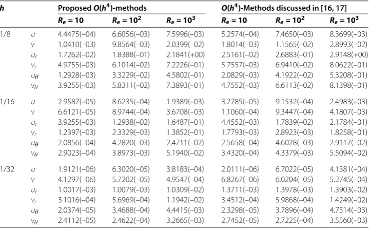
(b) In cylindrical polar coordinates inr-θ plane:
Figure 6 Exact and numerical solutions of the 2D Navier Stokes’ model equations in Cartesian coordinates.
The exact solution is given byu=rsinθ,v= rcosθ. (c) In cylindrical polar coordinates inr-zplane:
Re
urr+
rur+uzz–
ru
=uur+vuz+H(r,z), <r,z< , (.)
Re
vrr+
rvr+vzz
=uvr+vvz+I(r,z), <r,z< . (.)
The exact solution is given byu=rsinhz,v= –rcoshz.
HereRe> is called the Reynolds number. The MAE foru,vand their first order normal derivatives are tabulated in Tables - for various valuesRe. Figures , , give a com-parison of the plots of the exact and the numerical solutions to Example (a), (b) and (c) respectively.
7 Concluding remarks
Table 8 Example 8(a): Navier-Stokes’ model equations (58.1)-(58.2) in spherical polar coordinates inr-θplane
h ProposedO(h4)-methods O(h4)-Methods discussed in [16, 17]
Re= 10 Re= 100 Re= 500 Re= 10 Re= 100 Re= 500
1/4 u 4.0350(–03) 4.7668(–02) 1.0430(–01) 4.6880(–03) 5.3210(–02) 2.1678(–01) v 2.8464(–03) 2.4988(–02) 8.0180(–02) 3.6584(–03) 3.0824(–02) 8.8249(–02) ur 1.9901(–01) 6.1644(–01) 3.5356(+00) 2.7257(–01) 6.9552(–01) 4.3682(+00)
vr 4.8578(–02) 2.7314(–01) 2.0524(+00) 5.6682(–02) 3.5231(–01) 2.8934(+00)
uθ 1.4393(–02) 3.7298(–01) 2.0017(+00) 2.2692(–02) 4.5332(–01) 2.8126(+00)
vθ 1.1827(–02) 1.9936(–01) 1.0787(+00) 1.9770(–02) 2.7658(–01) 1.8655(+00)
1/8 u 4.5574(–04) 6.9580(–03) 2.4922(–02) 5.0324(–04) 7.3214(–03) 2.9911(–02) v 1.9624(–04) 2.9897(–03) 1.5191(–02) 2.4454(–04) 3.4789(–03) 1.9923(–02) ur 5.2907(–02) 8.0040(–02) 3.8376(–01) 5.7709(–02) 8.5140(–02) 4.3673(–01)
vr 1.2219(–02) 5.8063(–02) 3.1326(–01) 1.7912(–02) 6.3360(–02) 3.6623(–01)
uθ 1.7268(–03) 3.4954(–02) 2.1949(–01) 2.2862(–03) 3.9459(–02) 2.6444(–01)
vθ 1.5710(–03) 3.6024(–02) 2.0974(–01) 2.0017(–03) 4.1420(–02) 2.5479(–01)
1/16 u 2.6553(–05) 6.3235(–04) 2.4796(–03) 3.0355(–05) 6.6532(–04) 2.7697(–03) v 1.2965(–05) 3.0081(–04) 1.0288(–03) 1.5569(–05) 3.3180(–04) 1.3288(–03) ur 1.5887(–02) 1.5849(–02) 3.2901(–02) 1.9788(–02) 1.8948(–02) 3.5109(–02)
vr 3.1718(–03) 5.0558(–03) 3.4203(–02) 3.4817(–03) 5.3855(–03) 3.7302(–02)
uθ 1.2981(–04) 3.3899(–03) 2.5863(–02) 1.5189(–04) 3.6998(–03) 2.8368(–02)
vθ 3.2230(–04) 2.5193(–03) 1.7076(–02) 3.5032(–04) 2.8391(–03) 2.0670(–02)
Table 9 Example 8(b): Navier Stokes’ model equations (59.1)-(59.2) in cylindrical polar coordinates inr-θplane
h ProposedO(h4)-methods O(h4)-Methods discussed in [16, 17]
Re= 10 Re= 102 Re= 103 Re= 10 Re= 102 Re= 103
1/8 u 4.4475(–04) 6.6056(–03) 7.5996(–03) 5.2574(–04) 7.4650(–03) 8.3699(–03) v 1.0410(–03) 9.8564(–03) 2.0399(–02) 1.8014(–03) 1.1565(–02) 2.8993(–02) ur 1.7262(–02) 1.8388(–01) 2.1841(+00) 2.5161(–02) 2.6883(–01) 2.9148(+00)
vr 4.9755(–03) 6.1014(–02) 7.2226(–01) 5.7557(–03) 6.9410(–02) 8.0622(–01)
uθ 1.2928(–03) 3.3229(–02) 4.5802(–01) 2.0829(–03) 4.1922(–02) 5.3208(–01)
vθ 3.9255(–03) 5.8311(–02) 7.3893(–01) 4.7552(–03) 6.6113(–02) 8.1398(–01)
1/16 u 2.9587(–05) 8.6235(–04) 1.9389(–03) 3.2785(–05) 9.1532(–04) 2.4983(–03) v 6.6121(–05) 8.9744(–04) 3.6708(–03) 1.1060(–04) 9.3447(–04) 4.1807(–03) ur 3.9255(–03) 1.2938(–02) 1.6487(–01) 4.4552(–03) 1.7839(–02) 2.1784(–01)
vr 1.2397(–03) 2.3329(–03) 1.3852(–01) 1.7793(–03) 2.8923(–03) 1.8258(–01)
uθ 2.0856(–04) 4.2820(–03) 2.4711(–02) 2.5658(–04) 4.6028(–03) 2.9117(–02)
vθ 2.9023(–04) 3.8973(–03) 5.1940(–02) 3.4320(–04) 4.3379(–03) 5.5094(–02)
1/32 u 1.9121(–06) 6.3020(–05) 3.8183(–04) 2.0111(–06) 6.7022(–05) 4.1381(–04) v 4.1297(–06) 5.7202(–05) 4.9547(–04) 6.8267(–06) 6.0204(–05) 5.2745(–04) ur 1.0017(–03) 1.0079(–03) 1.0309(–02) 1.3711(–03) 1.3978(–03) 1.3903(–02)
vr 3.1016(–04) 5.6969(–04) 1.1942(–02) 3.4512(–04) 5.9868(–04) 1.4249(–02)
uθ 2.0374(–05) 3.4688(–04) 4.4415(–03) 2.3298(–05) 3.7896(–04) 4.7514(–03)
vθ 2.4112(–05) 2.4622(–04) 3.2665(–03) 2.7452(–05) 2.7225(–04) 3.5560(–03)
Table 10 Example 8(c): Navier-Stokes’ model equations (60.1)-(60.2) in cylindrical polar coordinates inr-zplane
h ProposedO(h4)-methods O(h4)-Methods discussed in [16, 17]
Re= 10 Re= 102 Re= 103 Re= 10 Re= 102 Re= 103
1/8 u 1.2914(–04) 1.1797(–03) 1.1198(–03) 2.0419(–04) 1.9997(–03) 1.9891(–03) v 2.4545(–04) 1.4028(–03) 2.5592(–03) 3.2445(–04) 2.1820(–03) 3.2295(–03) ur 6.7822(–03) 5.7549(–02) 5.6655(–01) 7.5228(–03) 6.5945(–02) 6.4556(–01)
vr 6.1035(–03) 5.5251(–02) 5.3119(–01) 6.8530(–03) 6.3152(–02) 6.1911(–01)
uz 4.7567(–04) 8.1710(–03) 8.9576(–02) 5.5765(–04) 8.8017(–03) 9.6675(–02)
vz 1.0385(–03) 1.8142(–02) 2.0159(–01) 1.4583(–03) 2.6241(–02) 2.8951(–01)
1/16 u 8.8980(–06) 2.0869(–04) 3.3219(–04) 1.2192(–05) 2.5968(–04) 3.8912(–04) v 1.4720(–05) 1.6494(–04) 4.2371(–04) 1.9882(–05) 2.1594(–04) 4.7173(–04) ur 5.4068(–04) 5.6217(–03) 4.8410(–02) 6.2860(–04) 6.1712(–03) 5.3014(–02)
vr 5.1521(–04) 4.6938(–03) 4.4798(–02) 5.6125(–04) 5.1839(–03) 4.9897(–02)
uz 9.6347(–05) 1.0593(–03) 7.7984(–03) 1.0743(–04) 1.5395(–03) 8.2489(–03)
vz 8.3467(–05) 1.1512(–03) 1.5110(–02) 8.8634(–05) 1.6215(–03) 2.0011(–02)
1/32 u 1.1626(–06) 1.6762(–05) 8.1323(–05) 7.4808(–07) 1.9267(–05) 8.4323(–05) v 9.0095(–07) 8.7775(–06) 8.2463(–05) 1.1469(–06) 9.0577(–06) 8.5364(–05) ur 1.1979(–04) 5.7479(–04) 5.8667(–03) 1.3778(–04) 6.0974(–04) 6.1764(–03)
vr 3.7573(–05) 3.4598(–04) 3.3449(–03) 4.0375(–05) 3.7895(–04) 3.6947(–03)
uz 1.9249(–05) 1.7590(–04) 4.3780(–04) 2.2942(–05) 2.0095(–04) 4.6086(–04)
vz 1.0944(–05) 8.8478(–05) 8.8297(–04) 1.2448(–05) 9.1874(–05) 9.1792(–04)
Competing interests
The authors declare that they have no competing interest.
Authors’ contributions
RKM discussed the difference method based on off-step discretization. NS discussed the convergence analysis of the method and the application of the proposed method to a diffusion equation and its stability analysis. NS also carried out all the computational work. All authors read and approved the final manuscript.
Author details
1Department of Applied Mathematics, Faculty of Mathematics and Computer Science, South Asian University, Akbar Bhawan, Chanakyapuri, New Delhi, 110021, India. 2Department of Mathematics, Faculty of Mathematical Sciences, University of Delhi, Delhi, 110007, India.
Acknowledgements
This research was (i) partially supported by the South Asian University, and (ii) partially supported by the Council of Scientific and Industrial Research under research grant No. 09/045(0903)/2009-EMR-I. The authors thank the reviewers for their valuable suggestions, which substantially improved the standard of the paper.
Received: 15 March 2013 Accepted: 8 July 2013 Published: 24 July 2013
References
1. Jain, MK, Jain, RK, Mohanty, RK: Fourth order difference methods for the system of 2-D nonlinear elliptic partial differential equations. Numer. Methods Partial Differ. Equ.7, 227-244 (1991)
2. Carey, GF: Computational Grids: Generation, Adaption and Solution Strategies. Taylor & Francis, Washington, DC (1997)
3. Yavneh, IV: Analysis of a fourth-order compact scheme for convection diffusion. J. Comput. Phys.133, 361-364 (1997) 4. Zhang, J: On convergence and performance of iterative methods with fourth order compact schemes. Numer.
Methods Partial Differ. Equ.14, 263-280 (1998)
5. Zhang, J: On convergence of iterative methods for a fourth-order discretization scheme. Appl. Math. Lett.10, 49-55 (1997)
6. Jain, MK, Jain, RK, Krishna, M: Fourth order difference method for quasi-linear Poisson equation in cylindrical symmetry. Commun. Numer. Methods Eng.10, 291-296 (1994)
7. Gupta, MM: A fourth-order Poisson solver. J. Comput. Phys.55, 166-172 (1984)
8. Gupta, MM, Manohar, RP, Stephenson, JW: A single cell high order scheme for the convection-diffusion equation with variable coefficients. Int. J. Numer. Methods Fluids4, 641-651 (1984)
9. Spotz, WF, Carey, GF: High order compact scheme for the steady stream function vorticity equations. Int. J. Numer. Methods Eng.38, 3497-3512 (1995)
10. Ananthakrishnaiah, U, Saldanha, G: A fourth order finite difference scheme for two-dimensional nonlinear elliptic partial differential equations. Numer. Methods Partial Differ. Equ.11, 33-40 (1995)
11. Saldanha, G: Technical note: A fourth order finite difference scheme for a system of 2D nonlinear elliptic partial differential equations. Numer. Methods Partial Differ. Equ.17, 43-53 (2001)
12. Erturk, E, Gökcöl, C: Fourth-order compact formulation of Navier-Stokes equations and driven cavity flow at high Reynolds numbers. Int. J. Numer. Methods Fluids50, 421-436 (2006)
13. Liu, J, Wang, C: A fourth order numerical method for the primitive equations formulated in mean vorticity. Commun. Comput. Phys.4, 26-55 (2008)
14. Ito, K, Qiao, Z: A high order compact MAC finite difference scheme for the Stokes equations: augmented variable approach. J. Comput. Phys.227, 8177-8190 (2008)
15. Li, M, Tang, T, Fornberg, B: A compact fourth-order finite difference scheme for the steady state incompressible Navier-Stokes equations. Int. J. Numer. Methods Fluids20, 1137-1151 (1995)
16. Mohanty, RK: Orderh4difference methods for a class of singular two-space dimensional elliptic boundary value problems. J. Comput. Appl. Math.81, 229-247 (1997)
17. Mohanty, RK, Dey, S: A new finite difference discretization of order four for (∂u/∂n) for two-dimensional quasi-linear elliptic boundary value problems. Int. J. Comput. Math.76, 505-576 (2001)
18. Mohanty, RK, Singh, S: A new fourth order discretization for singularly perturbed two dimensional non-linear elliptic boundary value problems. Appl. Math. Comput.175, 1400-1414 (2006)
19. Chawla, MM, Shivakumar, PN: An efficient finite difference method for two-point boundary value problems. Neural Parallel Sci. Comput.4, 387-396 (1996)
20. Stephenson, JW: Single cell discretization of order two and four for biharmonic problems. J. Comput. Phys.55, 65-80 (1984)
21. Varga, RS: Matrix Iterative Analysis. Springer, New York (2000)
22. Henrici, P: Discrete Variable Methods in Ordinary Differential Equations. Wiley, New York (1962) 23. Hageman, LA, Young, DM: Applied Iterative Methods. Dover, New York (2004)
24. Kelly, CT: Iterative Methods for Linear and Non-Linear Equations. SIAM, Philadelphia (1995) 25. Saad, Y: Iterative Methods for Sparse Linear Systems. SIAM, Philadelphia (2003)
doi:10.1186/1687-1847-2013-223