R E S E A R C H
Open Access
Synchronization of application-driven
WSN
Bruno Marques
1,2*and Manuel Ricardo
2Abstract
The growth of wireless sensor networks (WSN) has resulted in part from requirements for connecting sensors and advances in radio technologies. WSN nodes may be required to save energy and therefore wake up and sleep in a synchronized way. In this paper, we propose an application-driven WSN node synchronization mechanism which, by making use of cross-layer information such as application ID and duty cycle, and by using theexponentially weighted moving average(EWMA) technique, enables nodes to wake up and sleep without losing synchronization. The results obtained confirm that this mechanism maintains the nodes in a mesh network synchronized according to the applications they run, while maintaining a high packet reception ratio.
Keywords: Wireless sensor network (WSN), ContikiRPL, Nodes synchronization, EWMA
1 Introduction
Recently, there has been an increasing trend towards the deployment of WSN, where a large number of tiny devices interacting with their environments may be inter-networked and accessible through the Inter-net. For that purpose, several communication protocols have been defined making use of the IEEE 802.15.4 Physical and MAC layers [1]. The 6LoWPAN Network Layer adaptation protocol [2] is also used to enable the interconnection between low-power devices and the IP network. Since its release, the design of routing protocols became increasingly important [3] and RPL [4] emerged as the IETF proposed standard protocol for IPv6-based multi-hop WSN.
WSNs are constituted by sensor devices equipped with their own local clock for internal operations [5]. Events related to them, which include sensing, processing, and communication, are normally associated to timing infor-mation. In the particular case of WSNs, there are chal-lenges and factors related to node synchronization, which include low-cost clocks, effects of wireless communica-tion, and node failures. Moreover, WSNs are distributed and their nodes have multiple hardware and software con-straints such as low processing power, low memory and
*Correspondence: [email protected]
1Departamento Engenharia Eletrotécnica, Escola Superior de Tecnologia e Gestão, Instituto Superior Politécnico de Viseu, Viseu, Portugal
2INESC TEC, Faculdade de Engenharia, Universidade do Porto, Porto, Portugal
storage capabilities, and low-power consumption. These characteristics make time synchronization an important part of communication in WSNs, and synchronization protocols are required.
In [6], we presented a new paradigm, theapplication -driven WSN paradigm, as a cross-layer solution aimed to help reducing the energy consumed by a network of sensors executing a set of applications. This paradigm assumes that each application defines its own network and set of nodes so that the exchange of information can be confined to the nodes associated to the application. The nodes share information about the applications they run and their duty cycles.
In [7], we proposed an extension to the RPL routing protocol, theRPL-BMARQ, with the purpose of making the network aware of the traffic generated by applications. The main objective of this extension was to construct directed acyclic graphs (DAGs), by using information shared by the application and network layers, allowing the nodes to select parents by considering the applications they run. In that work, we characterized theenergy con-sumptionand theenergy gain and alsoend-to-end delay and fairness. For evaluation purposes, we selected four scenarios in which all the nodes joined the network at same time and performed simulations considering reg-ular RPL and RPL-BMARQ. Later, we started to study the behavior ofRPL-BMARQconsidering that the nodes would not join simultaneously the WSN. At this end,
we presented a draft of a possible node synchronization mechanism, and estimated the energy gains introduced by RPL-BMARQ.
In this paper, we consider a more realistic situation in which the nodes join the WSN at a non-predictable and different time. At this end, the sensor nodes must share some kind of time reference which allow them to be syn-chronized with respect to the life cycle of the applications they run. Therefore, in this paper, we propose a novel synchronization mechanismforRPL-BMARQ, which will help the nodes to wake up and to go asleep in a syn-chronized manner so that they can successfully send, receive, and forward packets, maintaining the energy consumption low.
The major contribution of this paper is then a mecha-nism for WSN which synchronizes the sensor nodes with respect to the applications life cycles they run, enabling these nodes to wake up and to go asleep in synchronism, while maintaining a packet reception ratio high. The nov-elty of our contribution comes from (1) the adaptation of the well-known exponentially weighted moving aver-agetechnique to wireless mesh network scenarios and (2) using this mechanism to control the behavior of sensor nodes so that they become synchronized in relevant time instants which are defined by their application duty cycles. The paper is organized in 6 sections. Section 2 presents the related work. Section 3 describes the application-driven WSN concept. Section 4 describes the ratio-nale of the contribution–the synchronization mechanism. Section 5 evaluates the proposed mechanism, describes the methodology adopted for its validation, and discusses the results obtained. Finally, Section 6 draws the conclu-sions and presents future work.
2 Related work
In this section, we present and discuss related work in three main areas:time synchronization, wake-up mecha-nisms for WSN, and 6LowPAN/IPv6/ RPL evaluations.
2.1 Time synchronization
WSNs are constituted by sensor devices equipped with their own local clock for internal operations [5]. Events related to them, which include sensing, processing, and communication, are normally associated to timing infor-mation. In the particular case of WSN, there are many challenges related to time synchronization because these networks are distributed by nature and because of the con-straints of the sensor nodes in terms of hardware and of software.
Akyildiz and Vuran [5] state that in order for the nodes to synchronize, they must exchange information about their clocks and use this information to synchro-nize their local clocks. By using wireless communications, WSNs create challenges for synchronization that result
from the error-prone communication nature of the wire-less channel which may cause packet losses due to low signal-to-noise plus interference ratios, or highly and vari-ant non-deterministic delays caused by MAC access and packet retransmissions. These factors affect also the time synchronization messages. Therefore, some nodes may be unsynchronized. On the other hand, synchronization messages sent by nodes may lead other nodes to adapt to their unsynchronized local clocks. As a consequence, the network may be partitioned into different areas with different time that prevents synchronization of the entire network. Also, the wireless channel may introduce asym-metric delays between two nodes, which is important for synchronization because some synchronization solutions depend on consecutive message exchange and round-trip-time delays. Therefore, robust synchronization methods are needed.
We start to identify some factors that influence the synchronization of the nodes and that should be consid-ered in the design of time synchronization mechanisms for WSN. As the Network Time Protocol (NTP) pro-tocol [8] is a synchronization propro-tocol normally used in IP networks, we provide an overview of it and also describe synchronization protocols for WSN related to our work.
2.1.1 Factors influencing time synchronization
According to [9], some of the factors influencing time synchronization in large systems constituted for example by personals computers, also apply to sensor networks, where temperature, phase noise, frequency noise, asym-metric delays, clock glitches, and sensors constraints are examples of these factors. In the case of the tempera-ture, since sensor nodes are deployed in various places, temperature variations throughout the day may cause the clock to speed up or slow down. In the case of thephase noisefactor, some of its causes are due to fluctuations in the hardware interface, response variation of the operat-ing system to interrupts, and jitter in the network. The frequency noise results from the instability of the clock crystal. In the asymmetric delayfactor, the delay of the path from one node to another node may be different from the return path which may result in an asymmet-ric delay and may cause an offset to the clock, which may go undetected. Clock glitches are abrupt jumps in time, caused by hardware or software anomalies such as frequency and time steps. Finally, WSN nodes are con-strained by nature because of limited resources (e.g., low in energy consumption, low in processing power, or low in memory).
problems introduced by the factors described above, avoid frequent message exchanges, and be self-configurable.
2.1.2 Network Time Protocol
The NTP [8] is the synchronization protocol more often used in the Internet. This protocol includes several syn-chronization mechanisms that have been also adapted for developed WSN synchronization protocols. Reference-broadcast synchronization (RBS) [10], timing-sync pro-tocol for sensor networks (TPSN) [11], lightweight tree-based synchronization (LTS) [12], and TSync [13] are some examples of these protocols. NTP is used to adjust the clock of each network node. This synchronization is achieved by using a hierarchical structure of time servers. The root node is synchronized with theCoordinated Uni-versal Time(UTC). In each level of this hierarchy, the time server nodes synchronize the clocks of their subnetwork peers. NTP uses a two-way handshake between two nodes to estimate the delay between these nodes and compute the relative offset accordingly (see Fig. 1, where nodeswill synchronize himself with noder). However, NTP assumes that the transmission delay between two nodes is the same in both directions. This is reasonable for the Internet, but some of the characteristics of WSN make this assumption inadequate. NTP is useful to discipline the oscillators of the sensor nodes, but using it to connect to time servers may be impossible because of sensor node failures, which are frequent in WSN. Using a single clock reference to synchronize all the nodes could be a problem due to the variations in network delays. Moreover, NTP requires intensive computing, requires a precise time server to syn-chronize the nodes, and does not consider the energy the nodes may spent to synchronize their clocks. All these problems may cause NTP to inaccurately measure delays and inaccurately estimate clock offsets.
2.1.3 Synchronization protocols for WSN
WSN poses unique challenges in the design of synchro-nization protocols, which calls for specific synchroniza-tion solusynchroniza-tions. An example is the effect of the broadcast wireless channel. However, wireless communication
Fig. 1NTP two-way handshake mechanism
introduce random delays between two nodes. Let us con-sider Fig. 2, which represents a handshake scheme. The delay between two nodes is characterized by four com-ponents: (i) the sending delay (tsend), (ii) the access delay
(tacc), (iii) the propagation time (tprop), and (iv) the
receiv-ing delay (trecv).
The handshake is initiated when nodesissues a SYNC packet with the timestampts1. Between the time the syn-chronization protocol issues the synsyn-chronization com-mand and the time during which the SYNC packet is prepared, there is a delay,tsend, resulting from the
combi-nation of operating system delays and transceiver delays on the node’s hardware;tacccorresponds to the additional
delay introduced by the wireless channel after the packet has been prepared and transferred to the transceiver. This delay depends on the MAC protocol when the node waits for accessing the channel; as an example, MAC pro-tocols using CSMA introduce a significant amount of access delay when the channel is very occupied.tprop is
the amount of time needed to transmit a SYNC packet to a receiver. Finally, trecv is the time required for the
transceiver of the receiver noderto receive the packet and process it. The transmission delay,ttx, is a component of the receiving delay, which is important and characterized by the time needed for the SYNC packet to be completely received (see Fig. 2); it depends on the transmission rate and on the length of the SYNC packet. These compo-nents contribute to the overall communication delay, also referred ascritical path. Delays are non-deterministic and create challenges when estimating clock offsets using the NTP’s methods. Most of the synchronization protocols for WSN tend to minimize the effects of these delays, which are random. In what follows, four related existing synchronization protocols are described.
Reference-broadcast synchronization: In Fig. 3, a sender-receiver handshake schemeis shown which intro-duces a significant amount of non-deterministic delay [10]. The RBS protocol tries to minimize the overall communication delay in the synchronization process. It eliminates the effect of the broadcast node. Instead of syn-chronizing the receiver with the sender, RBS synchronizes
1 2
3
4
5 6
7 m
m
m m m
m
Fig. 3Reference broadcast. Node 1 broadcastsmmessages which are used by the other nodes for synchronization purposes
a set of receivers that are within the reference transmis-sion of a sender. Considering that propagation times are negligible on wireless channels, as soon as a packet is transmitted, it is received at all sender’s neighbors almost at the same time. Therefore, the synchronization may be improved if only the receivers are synchronized. As shown in Fig. 3, node 1 broadcastsmreference packets and each one of the receivers, within its broadcast range, records the time the packets are received. Then, the receiver
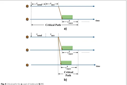
nodes communicate with each other to estimate the off-sets, just like the traditional synchronization. Figure 4a shows the critical path for traditional synchronization. Sending delays and the access delays should be accurately estimated to improve the synchronization. Reference-broadcast synchronization does not involve node 1 in the synchronization; only the receivers (nodes 2, 3, 4, 5, 6, and 7) synchronize among themselves based on a reference-broadcast message from node 1. As shown in Fig. 4b, this reduces the critical path duration. In fact, the possible origin of uncertainty in RBS is the time between when a broadcast packet is received and when it is completely processed.
A method used to determine with efficiency the clock offset of each node in relation to its neighbors is the receiver-receiver synchronizationmethod. By exchanging messages with each neighbor, a node fills a table consist-ing of relative offsets. Therefore, the main goal of RBS is not to correct the clocks of the nodes but, every time a packet is received, to translate its timestamp to the node’s clock using the relative offset information. This synchronization method can only provide synchroniza-tion in a broadcast area. In order to provide multi-hop synchronization, RBS uses nodes that receive two or more different reference-broadcast messages. These nodes are
calledtranslation nodes, and they are used to translate the time between different broadcast domains (see Fig. 5). As it can be observed, nodes A, B, and C are, respectively, the transmitter, the receiver, and the translation nodes. The transmitter node broadcasts its timing messages, the receiver node receives those messages, and then the nodes synchronize with each other.
Timing-sync protocol for sensor networks [11]: TPSN uses some of the NTP concepts: it uses a hierarchical structure to synchronize the entire WSN to a single time server. TPSN uses the root node to synchronize all or part of the network, consisting of two phases: (1) the discov-ery phase, where the structure of TPSN is built, starting from the root node and (2) the synchronization phase, where pairwise synchronization is performed across the network. In (1), the root node is assigned to level 0 and the other nodes in the network are assigned to levels according to their distance to the root node (see Fig. 6).
Firstly, the root node starts to construct the TPSN struc-ture. To this end, it broadcasts a special packet called level_discovery packet. In this structure, the first level is assigned to the number 0, which is the level of the root node. The other nodes that receive this packet are the nodes that belong to level 1. Afterward, these nodes broadcast their level_discovery packet. Then, the neigh-bor nodes receiving those packets are labeled as level 2 nodes, and the process is repeated until all the nodes in the network are assigned to a level.
In (2), each node in the structure is synchronized with a node from a higher level. The root node sends another packet (thetime_sync packet) which initializes the time synchronization process. Afterwards, the nodes in the
Fig. 5RBS multi-hop synchronization scheme
Fig. 6Synchronization architecture of TPSN
next level start to synchronize with the root node by send-ing a synchronization_pulseto it, as shown in Fig. 7. In order to avoid collisions with other nodes, each node in level 1 waits for a random amount of time before trans-mitting thetime_syncpacket. After the reception of this packet, the root node sends an acknowledgment back to finish the synchronization process. In this way, nodes belonging to level 1 of the structure are synchronized with root node (see Fig. 7). Thistime_syncpacket also serves as asynchronization_pulseto level 2 nodes. Upon a recep-tion of this packet from a node in level 1, the nodes in level 2 wait for a random amount of time for the level 1 nodes to finish their synchronization. Then, they initialize the synchronization process by transmitting a synchroniza-tion_pulse. Acting like the root node in level 0, a level 1 node sends back an acknowledgment, the process contin-ues until all the nodes at different levels are synchronized, and the entire network becomes synchronized.
In TPSN, the receiver synchronizes with the local clock of the sender according to the two-way message hand-shake, as shown in Fig. 7. For this reason, TPSN is based on asender-receiver synchronization method. Hierarchical structures created by TPSN are similar to the structures created by NTP. Like in NTP, nodes may fail causing nodes to become unsynchronized. Also, nodes mobility can make the hierarchy useless, as they may move out of their levels. Therefore, nodes at levelncannot synchro-nize with nodes at leveln−1, without requiring additional and periodical synchronization.
Lightweight tree-based synchronization [12]: LTS is similar to TPSN and follows two design approaches: cen-tralized and distributed. The cencen-tralized design is based on the construction of a tree such that each node is syn-chronized to the root node. After the tree is constructed, the root initiates pairwise synchronization with its chil-dren nodes and the synchronization is propagated along the tree to the leaf nodes.
In the distributed design, LTS does not rely on the con-struction of a tree and synchronization can be initiated by any node in the network. Each node performs synchro-nization only when it has a packet to send. Therefore, each node is informed about its distance (in number of hops) to the reference node for synchronization, the desired accu-racy, the clock drift, and a record of the time that has passed since they were synchronized. Then, the nodes adjust its synchronization rate accordingly. Nodes far-ther apart from the reference node perform synchroniza-tion more frequently because synchronizasynchroniza-tion accuracy is inversely proportional to distance.
In general, LTS is based on message exchanges between two nodes to estimate the clock drift between their clocks. This synchronization scheme is named pairwise synchronization scheme, and it is extended for multi-hop synchronization.
In contrast to our centralized and asynchronous pro-posed synchronization mechanism, in [14], a synchronous protocol is proposed that provides a distributed strat-egy which guarantees convergence for any undirected connected communication graph. This strategy tries to control the nominal clock period and the clock offset based on the information received from neighbor nodes in order to achieve synchronization. Moreover, when an underlying communication graph is known, the authors purpose an optimal design strategy which can be used to study the effect of noise and external disturbances on the steady-state performance.
There are additional works proposing and analyzing time synchronization mechanisms. In [15], the authors use factor-graph methods for network clock estimation and propose two methods for message passing: belief propagation (BP)andmean field (MF).
In [16], two joint synchronization and localization algo-rithms in both line of seeing (LOS) and in non-line of seeing (NLOS) environments are proposed. They applied Taylor expansions in order to represent factor graphs in closed Gaussian forms where the means and variances of beliefs of node estimates can be easily obtained by simple arithmetic operations.
In [17], the authors propose a global clock synchro-nization method by adopting apacket-based synchroniza-tion scheme. The proposed distributed algorithm requires communications only between neighboring sensors and computes a set of marginal distributions using the BP
message passing [18]. The authors have observed that the state of clock offset at any sensor depends directly only on its neighboring sensors and that the algorithm synchro-nizes clocks with a consistent reference value instead of adjusting clocks to an average value.
In [19], WSN time synchronization follows two strate-gies: (i)maximum time synchronization(MTS) to simul-taneously synchronize the skew and offset of each node when the communication delay is negligible and (ii) a weighted maximum time synchronization(WMTS) when the communication delay between the nodes is random. In contrast to our work, in which we synchronize a vir-tual clock, these authors attempt to synchronize the clock skew, in order to obtain acceptable synchronization accu-racies. The main idea of MTS and WMTS is to drive all clocks to the maximum value among the network. In [19], random communication delays with normal distribution are considered, while we validated our solutions against Gaussian and exponentially distributed delays. This solu-tion can be classified as distributed and asynchronous algorithm, whereas ours can be classified as centralized and asynchronous.
Since synchronization is a widely studied topic, in [20], a survey of clock synchronization for wireless sensor net-works is published.
2.2 Wake-up mechanisms for WSN
WSN are energy limited so typically the nodes cannot keep radios active all the time, having to sleep and to wake up periodically [21]. Addressing this issue, there have been proposed several MAC protocols which were categorized assynchronousorasynchronousMAC proto-cols. Although asynchronous protocols are simpler, they tend to consume more energy. But in WSN, where energy must be saved, a different approach may be used. One pos-sibility is to use synchronous methods. Using these proto-cols, some techniques are adopted to increase the nodes lifetime: (i)duty cyclingand (ii)scheduled rendezvous.
duty cycling techniques have been proposed. The S-MAC [24] and the T-MAC [25] protocols are examples of them. These protocols transmit aSYNCpacket to notify neigh-bors about their schedule and to synchronize the clocks of all nodes in the network. The method only compen-sates for clock offset and does not consider clock drift [21]. Moreover, the knowledgement of traffic patterns can also help to take decisions about waking up. This method is known as adaptive duty cycling. S-MAC [24] is one of the major energy-efficient MAC protocols that efficiently exploits the idea of adaptive duty cycling. It uses a periodic sleep-wake-up mechanism in order to lower power con-sumption. If a node has no packet to receive, it can waste a large amount of energy by just listening to the chan-nel. Consequently, a node can save a significant amount of energy if it simply goes to sleep mode by switching off its radios [22]. T-MAC is an improvement over S-MAC duty cycling. In the T-MAC, listening period ends when no event has occurred for a time thresholdTA. Though it improves on S-MAC, T-MAC has the disadvantage that it can face an early sleeping problem where a node can go to sleep even though its neighbor may still have mes-sages for it. Synchronization is also an issue in duty cycling MAC protocols. In [26], that synchronous MACs such as S-MAC have low energy consumption for sending packets but are complicated due to the need of synchronization is argued. Conversely, asynchronous MACs, for example WiseMAC [27], is very simple, but it spends much energy in finding the neighbor’s wake-up time. Moreover, syn-chronous methods can be characterized as one-way meth-ods. Usually, the senders broadcast a reference message and receivers, upon the reception of the message, record the arrival time by their own clocks, and exchange this information among each other to compensate clock offset between them. In [21], a synchronous method is pro-posed in which clocks in the all network are not modified. Instead, the nodes are synchronized with their own clocks. Since the periodic broadcast event in the network is the same, although they have different measurement results for this period by their own clock unit independently, they are able to interact with each other at the same physical time. Without complicating the estimation process and without modifying the clock of a node, this synchroniza-tion method becomes simpler and more energy-efficient than the traditional synchronization one-way method.
Scheduled rendezvous: This type of MAC protocol requires a prescheduledrendezvoustime at which neigh-boring nodes wake up simultaneously. In this method, a node wakes up periodically and sleeps until the next ren-dezvous time. Ascheduled rendezvousscheme is shown in Fig. 8 [22].
The advantage of this scheme is that when a node is awake, it is guaranteed that all its neighbors are awake
Fig. 8A scheduled rendezvous scheme
as well. Consequently, it is easier to send/receive pack-ets. Broadcasting a message to all neighbors is also sim-pler in scheduled rendezvous schemes. RI-MAC [28] is areceiver-initiatedasynchronous duty cycle MAC proto-col for WSN. It uses a receiver-initiated data transmission in order to proficiently operate over a wide range of traf-fic loads. It attempts to minimize the time a sender and the receiver occupy the medium to find a rendezvous time for exchanging data, while still decoupling the sender and receiver’s duty cycle schedules. A disadvantage of such MAC protocol is the requirement to maintain strict syn-chronization because clock drifting may deeply affect the rendezvous time.
2.3 6LowPAN/IPv6/RPL evaluations
In [29], a cross-layering design for RPL which provides enhanced link estimation and efficient management of neighbor tables is proposed. They used AMI as a case study and employed theCoojaemulator to evaluate their proposal. The authors analyzed RPL together with the underlyingX-MAC andContikiMAC andNullrdc proto-cols from the reliability stand point by consideringpacket loss,end-to-end delay, andenergy consumptionand have implement a testbed using ContikiOS to validate their work. In [30], the performance of RPL used for multi-sink WSNs considering thehop-countand/orETX, packet loss, and energy consumption metrics is evaluated. To validate the results from the performed simulations, the authors performed on a real-life testbed the same tests.
end-to-end packet delay, energy consumption, query suc-cess ratio, and fairness Index. Query sucsuc-cess ratio (QSR) quantifies the success of a sink node with respect to the reception of all the expected reply packets upon the trans-mission of a query packet; this metric allows us to see if all the nodes receive the query packets and if they reply back. Therefore, it is easy to verify packet loss. The fair-ness index metric is used to investigate if the nodes have the same opportunity to reply back to the sink. We used ContikiOS/Cooja for the simulations and validated our work by implementing two testbeds.
3 Application-driven WSN
Theapplication-driven WSN paradigm [6] assumes that each application defines its own network and set of nodes so that the exchange of information can be confined to the nodes associated to the application. The nodes share information about the applications they run and their duty cycles, and nodes are put asleep when there is no activ-ity related to their applications. When nodes receive a query packet, they know exactly when they must wake up on the next period. The nodes alternate between wake and sleep states, and the amount of time spent in each phase is determined by the application duty cycle. When the wake-up time expires, the node switches to the sleep state, waking up again by the time computed by the synchronization mechanism proposed in Section 4 of this paper.
We assume that every node can participate in route discovery and packet forwarding. However, the nodes for-warding a given type of data will be primarily selected from the set of nodes running the same application to which the data is associated. For that purpose, each query packet includes information about the associated
application (APPID), which is known by the nodes run-ning that application. Our routing scheme tries to insure that data of an application is relayed mainly by the nodes running that application. When the sink node queries the other nodes running the same application, routing paths follow the directed acyclic graph (DAG) created. This DAG is created and maintained by a change to the RPL protocol scheme which uses mainly the nodes running that application; the nodes not associated to this applica-tion will not participate in the routing process, in a first attempt. In our proposal, the subset of nodes running the same application forms a “subnetwork” with multi-hop connectivity and application packets carry out also infor-mation about the application duty cycle (TCYCLEandTON)
that is used to create and maintain the DAGs in which not only the nodes running the same application but also the nodes having the same application duty cycle can be “grouped”. Figure 9a shows a network topology support-ing two different applications. Figure 9b shows the DAG created with standard RPL, and Fig. 9c shows the DAG created by our proposed solution. The wake-up mecha-nism is based on the applications time cycle information (TCYCLEandTON), carried by every application query sent
by the sink nodes. When a node receives a query packet, it knows exactly when it must wake up on the next period.
4 Application-driven synchronization mechanism According to our application-driven concept, synchro-nization is achieved between the nodes that run the same applications or between the nodes that have the same application duty cycle, by considering their duty cycles. Therefore, the first time a node joins the network, it waits for an application query packet to adjust its virtual clock to the time carried by the query packet. We realize that this
a)
corresponds to setting the time’s nodes to a value which does not consider network delays but, as demonstrated in the paper, this has no impact on our synchronization mechanism as the nodes dynamically adjust their sleep-ing offset (see β · |δk,n| component in Eq. 2) and wake up and sleep almost at the same time during the network lifetime. As such, the synchronization algorithm takes advantage of the application query packets that are sent by the sink nodes once in every application duty cycle to maintain the sensor nodes synchronized. A network may support several applications but only the nodes run-ning the same application or having the same duty cycle will synchronize between them. Therefore, a network sup-porting different applications may have different sets of nodes with different synchronizations and still be fully functional. Without having to send or to receive other type of packets for synchronization purposes, the nodes will rely only on the queries received to synchronize. In fact, this algorithm is centralized on a sink node, but its design is simple and adequate for our purposes. A dis-tributed design would be more complex and imply the use of other types of packets for synchronization, often broad-casted through the network, which would have impact in energy consumption due to packet transmission and reception costs.
It is unlikely that all the sensor nodes would join a net-work at the same time. Having the nodes active all the time would deplete their batteries, so the nodes have to go sleep and to wake up periodically. All the nodes have to be awake almost at the same times in order to receive sink queries and to forward them to the other nodes. As a result, the nodes must be synchronized according to the application cycle they run. In order to synchronize all the nodes in the network, our proposed synchronization mechanism uses a synchronous method which includes two phases:the synchronization setup phaseandthe syn-chronization maintenance phase, described below.
4.1 The synchronization setup phase
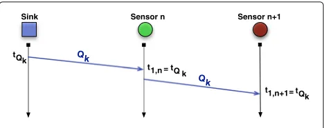
When a sensor node joins the network, it remains in the wake state and waits for the reception of its first query packet sent by the sink node and forwarded by other nodes. Upon its reception, the node adjusts a vir-tual clock to the timestamp carried by the query. As it can be observed from Fig. 10, the query packet sent by a sensornode n towards a sensornode n+1 is the same query packet that node n received from the sink node. The timestamp carried by the query is extracted from the query packet. This phase is used to readjust the vir-tual clock; the periodicity of this readjustment depends on how often the nodes have to readjust their virtual clock. It is known that this phase corresponds to setting the time’s nodes to a value which does not consider network delays.
Sink Sensor n Sensor n+1
Qk
tQk
t1,n = tQk
Qk
t1,n+1= tQk
Fig. 10Synchronization setup phase
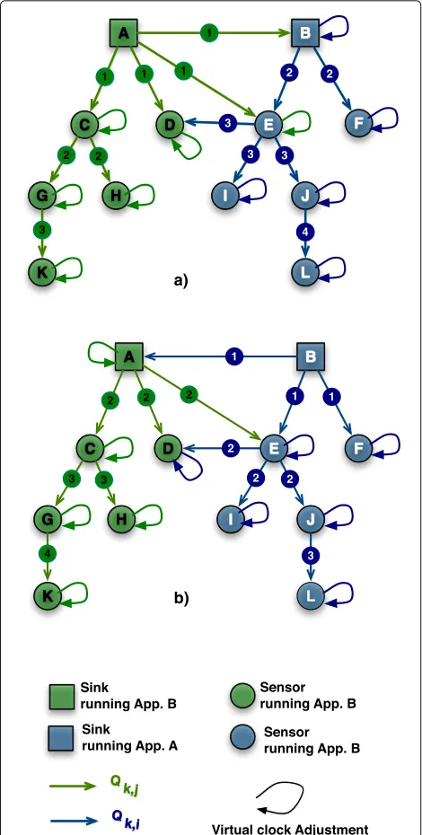
In the example shown in Fig. 11a, sink node A issues a query (Qk,j) before sink node B. The query packet is disseminated through the network as expected using the RPL-BMARQrouting solution [7]. Sensor nodes C and D, which run this sink’s application, set their virtual clock to the timestamp carried out by the packet. Sensor node E, not running this application, also sets his virtual clock to the timestamp carried out by the query packet since it is the first query it receives. The same query packet (Qk,j) is then forwarded to the other sensor nodes (nodes G, H, and K) which will also set their virtual clock to the same timestamp. Sensor node E will not forward the query packetQk,jsince it does not run this application and does not have neighbors running it. Similarly, node F, upon the first query packet (Qk,i) reception from sink node B, and because it runs the same application, adjusts it virtual clock to the time carried out by the sink B query packet. As this sink has already adjusted its virtual clock using the sink A timestamp, sensor node F will have the same time as the other nodes. Again, the queryQk,iwill be forwarded to the other sensor nodes (nodes I, J, and L) which will per-form the same virtual clock adjustment. Figure 11b shows the same virtual clock adjustments, but in this case, it is sink node B that issues the first query packet and adjusts all the network node’s virtual clocks.
4.2 The synchronization maintenance phase
Since all the nodes know the characteristics of the appli-cations they run, after the reception of the first query packet, they expect to receive the second query packet by t2 = t1+TON +TOFF. The time the nodes are
sleep-ing (TOFF) is defined asTCycle−TON whereTCycleis the
application duty cycle time andTONis the time the nodes
are awaked during each duty cycle. However, because net-work delays are variable, the nodes will receive this second query packet not int2 but int2, as shown in Fig. 12. There
is a difference between the expected valuet2 and the real valuet2,δ2 = t2−t2. For example, if a node is expected
to receive a query packet by t2 = 100 and receives it by t2 = 102, then δ2 = −2. A negative value means
a)
b)
Fig. 11Example of nodes synchronization
query packet reception and characterized by the sum of the processing and queueing delays in intermediate and destination sensor nodes, and the transmission delays and propagation delays in intermediate nodes. An in-depth characterization of these delays may be found in [31].
Our proposed mechanism estimates δk,n by using the exponentially weighted moving average (EWMA) tech-nique (see Appendix). According to Fig. 12, the difference between the expected time to receive the next query and the time it is really received is computed by Eq. 1:
tk,n = tk−1,n+TON+TOFF
δk,n = (1−α)·δk−1,n+α·(tk,n−tk,n); 0 < α < 1
(1)
wheretk,n is the expected packet reception time andtk,n is the real packet reception time.δk,nis evaluated accord-ing to EWMA as in Eq. 3 withαreflecting the weight of the last observation. Theδk,nvalue is dynamically adjusted every time a node wakes and receives a query packet, and it is used to control the time the node would sleep in the next cycle, given by Eq. 2.
TSleepk,n =TOFF−β· |δk,n| (2)
In Eq. 2, theβ factor is used to amplify theδk,n value to guarantee that the sensor node will wake some time before the next application cycle.β · |δk,n| is the sleep-ing offset and represents the time the node will wake up before the start of the next application duty cycle. Algorithm 1 shows the pseudo-code of the application-driven synchronization mechanism with values given toα andβand to the virtual clock adjustment periodicity time (adjust_periodicity_time).
Algorithm 1: Pseudocode of the proposed synchro-nization mechanism
foreach(app.querykreceived)do
α=0.125;
β=10;
if(first(app.query))then set_clock(query→TTX);
adjust_periodicity_time = 3600·24 (eg. 24 hours);
adjust_counter = adjust_periodicityT _time
CYCLE ;
else
if(app.query_id == node.app_id)then t’k,n= tk−1,n+ TON+ TOFF; tk,n= node.queryTRX;
δk,n=(1−α)·δk−1,n+α·(tk,n−tk,n);
TSleepk,n= app.TOFF-β· |δk,n|; adjust_sleep_timer(TSleepk,n);
adjust_counter = adjust_counter - 1; end
if(adjust_counter == 0)then set_clock(query→TTX);
adjust_counter =adjust_periodicityT _time
CYCLE ;
Sink Sensor n Sensor n+1
Q 1
t 1 Q1
t1,n=t1
t 1 TON TOFF
+
+
Q2
Q2
t2,n
t2,n+1
t'2,n+1=t1,n+1+TON TOFF+ t'2,n =t1,n+TON TOFF+
2,n
2,n+1
t1,n+1= t1
Fig. 12Synchronization maintenance phase
5 Evaluation
In order to validate this mechanism, first we present a study on how the nodes can maintain their synchroniza-tion by estimating and evaluating the parameters pre-sented in Eqs. 1 and 2, which corresponds to investigate in depth the synchronization maintenance phase. We also present and discuss results from the proposed synchro-nization mechanism using different values for α andβ parameters, and query success ratio (QSR) results from simulations, and finally present and discuss some of the results obtained from two real testbeds. The QSR metric is defined as the ratio between the number of reply pack-ets received by a sink node in response to a query packet and the number of replies the sink expects to receive.
5.1 Basic simulation of the synchronization mechanism The node synchronization mechanism was evaluated considering the following probabilistic distribution of net-work delays: (1) uniform distribution, (2) Gaussian distri-bution, and (3) exponential distribution.
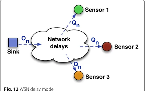
Figure 13 shows one sink node and three sensor nodes. The sink node transmits queries regularly. Each query time reception is affected by those different network delays, and the sensor nodes upon their reception will adjust their sleep time in order to try to wake up at same time on the next application duty cycle. For each node, dif-ferent mean delays were considered: sensor node 1, 0.5 s; sensor node 2, 1 s; and sensor node 3, 2 s.
A Python program was written in order to randomly generate different network delay distributions. The pro-gram generates 105queries, uses Eq. 1 to estimate the new
expected query reception time by each node, and uses it to adjust the time each node must sleep (Eq. 2) in order to wake up on time for the next application cycle. Finally, the program computes how many time the nodes are waked
up simultaneously. We consider that nodes are simulta-neously awaked up if the three sensors are awaked for at least=80%·TON. Let us also defineTSensorsONas a
ran-dom variable which captures the time during which the three sensors are simultaneously on the ON state, having valuesTSensorsON[0s,TONs] (see Fig. 14). An occurrence
ofTSensorsONis computed as the time the first sensor goes
asleep minus the time the last sensor wakes up.
In a first attempt, forα in Eq. 1, the value was set to 0.125, following current IETF recommendations for man-aging TCP timers [32], and for Eq. 2, the β value was empirically set to 10. All the sensor nodes wake every 15 min remaining waked for 1 min (TON = 60 s and TOFF=840 s).
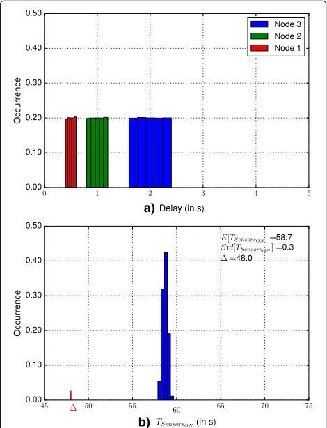
Figure 15 shows results for the first situation evaluated—uniformly distributed network delays, with delays varying between ±20% × 0.5 s, ±20% × 1.0 s, and ±20% × 2.0 s. In Fig. 15a, one can see the his-togram of randomly generated delays; Fig. 15b shows TSensorsON’s histogram. Again, we can observe that
t 1
2
3
TON
TSleep
TSensorsON Fig. 14Nodes adjustment ofTONsimultaneity
P[TSensorsON ≥ ]= 1. In fact, it is verified that
TSensorsON[57.88, 59.66] s, and the mean value of
E[TSensorsON]= 58.7 s. As in the first situation, the nodes
maintain synchronism in all the cycles.
Figure 16 shows results for the second situation evaluated—Gaussian distributed network delays, with delays having a standard deviation which is 20% of the mean values which are 0.5, 1.0, and 2.0s respectively. In
a)
b)
Fig. 15Uniformly distributed network delays.aDelay histogram.b
TSensorsON’s histogram
a)
b)
Fig. 16Gaussian distributed network delays.aDelay histogram.
bTSensorsON’s histogram
Fig. 16a we can observe the histogram of randomly gen-erated delays; Fig. 16b shows TSensorsON’s histogram. As
it can be observed,δk,nfactor from Eq. 2 also affects the time each node must sleep (TSleepk,n). Similar to the
previ-ous cases,P[TSensorsON ≥ ]= 1, and the mean value is
E[TSensors]= 58.77 s. In this situation the nodes will also
maintain synchronism in every application cycle.
Figure 17 shows results from the last situation evaluated—exponentially distributed network delays, with mean delays targeting 0.5, 1.0, and 2.0 s, respectively. In Fig 17a, the histogram is shown and, as expected, there are variations; Fig. 17b showsTSensorsON’s histogram. As can
be observed, there are situations where the success con-dition is not satisfied. In this case,E[TSensorsON]= 57.52 s
andTSensorsON[25.06, 59.99] meaning that the nodes will
a)
b)
Fig. 17Exponentially distributed network delays.aDelay histogram.
bTSensorsON’s histogram
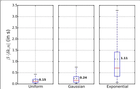
TOFF−1.11s. Moreover, results showed that the
proba-bilityP[TSensorsON ≥ ]= 1 is observed in 99% of the
occurrences, which means that all the considered nodes will be active at same time during at least=80%·TON
in 99% of the application’s duty cycles.
The box plot figures in this paper give the standard metrics: the 25th percentile, the 75th percentile, and the red line is the median value. The top and bottom of
Fig. 18Box plot forβ· |δk,n|, the sleeping offset represented in Eq. 2
the whiskers show the maximum and minimum values, respectively. Finally, the black dashed line in the box represents the mean value.
From this analysis, we may conclude that the synchro-nization mechanism may be adequate for our purposes. In order to increase the trust in these results, a sensibil-ity analysis is also carried out, in order to understand how TSensorsONis affected by different values ofαandβ.
5.1.1 αandβvalues estimation
We performed studies using different values for the synchronization mechanism parametersαandβ. We con-sidered four sensor nodes and assumed a uniformly dis-tributed delays varying in ±20% ×0.5 s, ±20%×1.0s,
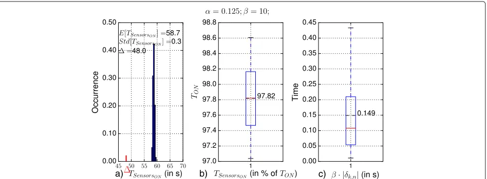
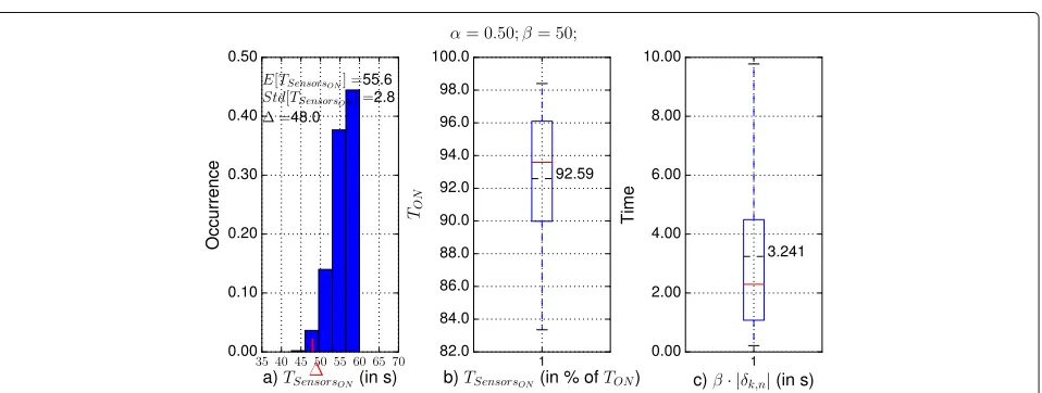
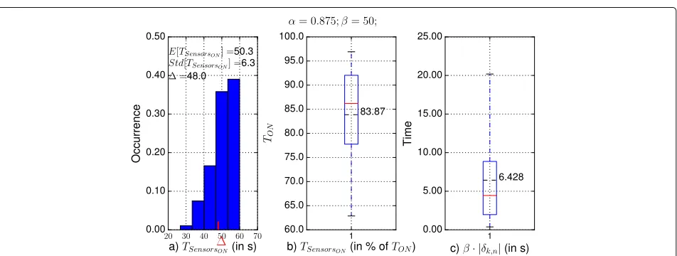
±20%×2.0s. Figures 19, 20, 21, 22, 23, 24, 25, 26, and 27 show the results obtained when considering different val-ues for the α and β parameters. Each of these figures present: (a) theTSensorsON’s histogram; (b) the box plot for
TSensorsON(in % ofTON); and (c) the box plot forβ· |δk,n|.
In the sensibility analysis shown below, we select two discrete set of values forαandβ,α ∈ {0.125, 0, 5, 0.875} andβ ∈ {1, 10, 50, 100}. We vary one parameter at time while maintaining the other constant.
αestimation: the weight given to the last sample in the calculation δ. Therefore, we want to investigate how it affects the synchronization mechanism by givingα differ-ent values, namely 0.125, 0.50, and 0.875.
βestimation since theδk,nvalue from Eq. 1 is small, we amplify it. The amplifying factor is theβparameter, and for it, we selected three values,β ∈ {10, 50, and 100}.
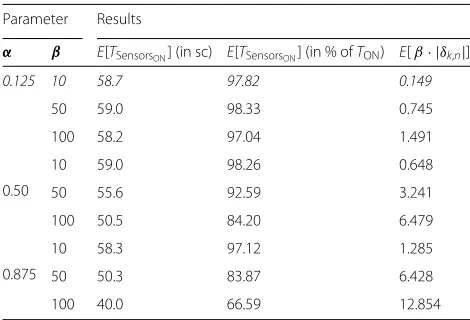
Figures 19, 20, 21, 22, 23, 24, 25, 26, and 27 show the results obtained for different combinations of the parame-ter’s values. Table 1 summarizes it, showing: (a) theαand
β values, (b) theE[TSensorsON], (c) averageE[TSensorsON]’s
time in % of TON, and (d) E[β · |δk,n|] component, the resulting sleeping offset.
For the selection of the α and β values, we consid-ered the values that satisfy at the same time: (i) values of TSensorsONin % ofTONabove 80% and (ii) lowestβ· |δk,n|
component value. Italicized values correspond to the ones that better satisfy our purposes.
5.1.2 Results discussion
This analysis of the results showed that not all the values chosen forαandβparameters satisfy our synchronization mechanism requirements. In fact, if we consider, respec-tively,α = 0.50 and β ∈ {50; 100}, the mechanism will fail because the probabilityP[TSensorsON ≥ ]< 1 (see,
a) b) c)
Fig. 19Uniformly distributed network delays withα=0.125;β=10.aTSensorsON’s histogram.bBox plot forTSensorsON(% ofTON).cBox plot for β· |δk,n|
a) b) c)
Fig. 20Uniformly distributed network delays withα=0.125;β=50.aTSensorsON’s histogram.bBox plot forTSensorsON(% ofTON).cBox plot for β· |δk,n|
Fig. 22Uniformly distributed network delays withα=0.50;β=10.aTSensorsON’s histogram.bBox plot forTSensorsON(% ofTON).cBox plot forβ·|δk,n|
Fig. 23Uniformly distributed network delays withα=0.50;β=50.aTSensorsON’s histogram.bBox plot forTSensorsON(% ofTON).cBox plot forβ·|δk,n|
Fig. 25Uniformly distributed network delays withα=0.875;β=10.aTSensorsON’s histogram.bBox plot forTSensorsON(% ofTON).cBox plot for β· |δk,n|
Fig. 26Uniformly distributed network delays withα=0.875;β=50.aTSensorsON’s histogram.bBox plot forTSensorsON(% ofTON).cBox plot for β· |δk,n|
Table 1Summary of synchronization mechanism results as a function ofαandβ
Parameter Results
α β E[TSensorsON] (in sc) E[TSensorsON] (in % ofTON) E[β· |δk,n|]
0.125 10 58.7 97.82 0.149
50 59.0 98.33 0.745
100 58.2 97.04 1.491
0.50
10 59.0 98.26 0.648
50 55.6 92.59 3.241
100 50.5 84.20 6.479
0.875
10 58.3 97.12 1.285
50 50.3 83.87 6.428
100 40.0 66.59 12.854
we can observe that there are occurrences forTSensorsON
below 80%, the threshold established for success, being in average equal to 97.82% ofTON. Therefore, those values
do not satisfy our selection criteria. From the other values evaluated, we may consider thatα = 0.125 andβ = 10 are the values that better satisfy our purposes, for the sce-narios considered. Comparing to other pair of values for
αandβ, these values present at the same time (i) greater TSensorsONvalue (58.7), which is almost the same
theoret-ical value ofTON; (ii) all the occurrences forTSensorsONin
terms ofTON% are above 97%, being in average equal to
97.82%; and (iii) the meanβ·|δk,n|component has, in aver-age, the lowest value 0.149 what means that the sensor nodes have to wake up before the next duty cycle less time than in the other cases. This will have impact in energy consumption since the sensor nodes do not have to stay unnecessary time awaked.
5.2 Simulations
In [6] and in [7], two different applications were used in three different scenarios, being the nodes distributed
as shown in Fig. 28. Simulations ran in Contiki’s Cooja simulator [33]. All the nodes are within a distance of 25 m for a transmission range of 30 m and support one of the two applications. Each application is running in eight nodes, and each node runs a single application. In scenario 1, the nodes running App. A were selected in a way that a long path could be obtained; in scenario 2, both applications have the same node distribution; sce-nario 3 is used to investigate situations where at least one node from other application is required to relay data. Let us, for example, consider Fig. 28c. In this sce-nario, we can observe that node 9 routes/forwards packets of an application that it does not run. In the scenarios simulated, sink nodes are always awake, and sink node running App. B (node 9) was chosen as the network DAG root because of its application duty cycle. For the nodes running application A, TON = 60 s, TOFF =
3540 s; for the nodes running application B,TON = 60 s, TOFF=840 s.
We simulated two situations: (i) a situation where all the nodes join the network at the same time, so that the pro-posed synchronization mechanism is not used as, in sim-ulations withCOOJA, clock drifting is the same for all the sensor nodes and (ii) the nodes will join the network at dif-ferent times. The later implies the use of the synchroniza-tion mechanism described in Secsynchroniza-tion 4 in order to keep the nodes synchronized with respect to the applications they run. The nodes join the network at different times which were randomly generated between 317 and 1102 s.
5.2.1 Results and discussion
In [34], the authors noticed timing inaccuracies in com-parison to experiences made on TelosB motes hardware. Their simulations showed unexplained delays during packet transmission (TX) over the radio medium that were not observed during similar experiences on physical motes. According to their investigations, they discovered that the problem is with the emulation of
MSP430-a) b) c)
Fig. 29Box plot forβ· |δk,n|, withα=0.125 andβ=10, for each hop in scenario 1
powered, radio-enabled WSN motes by the MSPSim soft-ware package when loading packet data into the transmis-sion buffer. The emulating mote performs this TX buffer loading at a different speed than the actual hardware. This may result in inexact simulations results. Nevertheless, the authors argue that, for the WSN application studied, time precision is not a key issue since the applications are not designed for real-time critical applications. The authors have selected the TelosB Hardware platform and ContikiOS/Cooja because there is no need to write the code twice since it is the same for physical motes and emulated motes, and the TelosB platform is the most used platform in the academia. This time inaccuracy has no impact in our synchronization mechanism. The EWMA technique used to control the synchronization of the sensor nodes also considers the resulting unex-plained delays during packet transmission to estimate the arrival of the next query packet, and the simula-tion and testbed results show that the synchronizasimula-tion mechanism performs well when having different network delays.
In our solution, each time a node receives a query, it computes the time it must wake up before the start of the next application cycle in order to be able to receive and forward packets and to successfully reply back to the sink.
The synchronization mechanism was configured withα= 0.125 andβ=10.
In the simulations, 16 nodes have been used, half of them running each application. Each scenario was simu-lated ten times, and information was extracted in order to estimate delays,QSR, and theE[β·|δk,n|] component. The results obtained are the following.
Delays We considered delayas the sum of all per-hop delays for each sensor query packet reception and charac-terized by the sum of the processing and queueing delays in intermediate and destination sensor nodes and the transmission delays and propagation delays in intermedi-ate nodes.
Per hopβ· |δk,n|component: From the simulations, we have extracted information about theβ· |δk,n|component on a per-hop basis. Fig. 29 shows the box plot for this component in scenario 1. We can observe that, except for the first hop, this component presents per hop similar val-ues, and sensor nodes would have to wake with an average sleeping offset of about 0.232 s. In the first hop, the sleep-ing offset has a grater value (0.49 s in average) because in this hop, we can observe some congestion, particularly between the sink node (node 1) and the sensor node 2.
Fig. 31Box plot forβ· |δk,n|, withα=0.125 andβ=10, for each hop in scenario 3
Figure 30 shows the box plot for theβ · |δk,n| compo-nent in scenario 2. As in scenario 1, we can also see that this component presents similar values per hop, with an average sleeping offset of about 0.176 s.
Finally, Fig. 31 shows the box plot for theβ· |δk,n| com-ponent in scenario 3. As in the other two scenarios, we observed that this component presents similar values per hop, in an average of about 0.242 s. In the case of the sleeping offset for two hop nodes, it has in average a grater value (0.35 s). Analyzing this scenario’s topology, and the traffic that may occur, we can observe some con-gestion around sensor nodes 3 and 13. For sensor node 3, it needs to forward replies from sensor nodes 4, 7, and 8. For sensor node 13, it also forwards replies from sensor nodes 11, 12, 14, 15, and 16. However, this sleeping offset value can be also considered as negligible as it has a small additional value.
In Fig. 32, the box plot for the expected sleeping off-set value for each of the three scenarios studied is shown. As it can be verified, the nodes would sleep not theTOFF
time, but in averageTOFF−0.716 s. Moreover, we observed
that, independent of the network topology, this compo-nent has almost the same values, what confirms that the synchronization mechanism proposed is adequate for our
Fig. 32Box plot forβ· |δk,n|, withα=0.125 andβ=10, for each scenario (in s)
purposes. Moreover, comparing the results from Figs. 34 and 35, we observe that for scenarios 2 and 3, the max-imum and minmax-imum β · |δk,n| values are different. In scenario 2, the nodes have more neighbors running the same application, what implies that each of them may need more time to access the wireless medium to forward a query. This is also reflected on the network delays and affects theβ· |δk,n|component.
QSR: Fig. 33 shows the box plot forQSR. In this figure,(1) the results using the standardRPL routing protocol, (2) the results usingRPL-BMARQ solution proposed in [7] without the synchronization mechanism implemented, and (3) the results using the sameRPL-BMARQsolution fully implemented are showed. As it can be observed, in average, 98.8% of the queries sent by sinks are replied by sensor nodes. With this success ratio, we can argue that the quality of the proposed synchronization mechanism is confirmed.
5.3 Testbed experiments
In order to confirm the results obtained from theoretical studies and simulations, we also tested our proposed solu-tion in a real environment. For that purpose, two of the scenarios studied were selected (scenarios 1 and 3) and
Fig. 34Scenarios deployed.aDeployment 1.bDeployment 2
deployed. Since it was not possible to reproduce them at the same scale, the scenarios deployed correspond to a 3×3 square lattice topology, while keeping all the other functionalities. In order to obtain reliable terms of com-parison, we have simulated these deployments using the same methods as in Section 5.2 and compared the sim-ulated results with those obtained in testbeds. Figure 34 shows both topologies deployed and simulated, which were realized usingTelosB motes[35], placed at distances of 5 m, and the radio transmission power was reduced to
−7 dBm in order to reduce the node reception distance. Application A run in five nodes (1, 2, 3, 4, and 5), and application B runs in four nodes (9, 10, 11, and 12). Node 9 is, at the same time, the root of the DAGs and a sink. Node 1 is the other sink. The nodes ranContikiOS(2.6) [36] which is an operating system for WSN which incor-porates an implementation of theIPv6protocol stack and usesRPLas the default routing protocol.
5.3.1 Results and discussion
Each testbed experiment was carried out for 4 h. To log real-time data, two Raspberry Pi platforms were used, connected to both sink nodes via a serial connection. Inside each Raspberry Pi [37] platform was a python pro-gram running, responsible to get timestamp data from each sink with respect to query packets sent and reply
Fig. 36Box plot forβ· |δk,n|, withα=0.125 andβ=10, for each deployment (in s)
packets received. In order to verify our proposed syn-chronization mechanism, we considered in this work (i) synchronization parameter’s valuesα = 0.125 andβ = 10; (ii) packet reception time on the sink nodes side to estimate the expected reception time and to compute the sleeping offset component (β· |δk,n|); and (iii)QSRresults. The main results obtained include the following:
β· |δk,n] component: Figure 35 showsβ · |δk,n| compo-nent, the sleeping offset represented in Eq. 2 histogram for each deployment. As expected, it presents the same uni-form distribution characteristics as the theoretical evalu-ation and the simulevalu-ations performed. Moreover, we can see in Fig. 36 that this component presents in average a sleeping offset of 0.185 s.
QSR: Figure 37 shows simulation and real implementa-tion results. As it can be seen, both present same values (100%), which means that also in real testbeds, the nodes reply to all the queries sent by sinks, going to sleep and waking up while being synchronized.
From the above results, we can conclude that there are no major differences between what was observed in
Fig. 37Query success ratio (QSR) for the scenarios deployed (in %)
the theoretical studies and in the simulation environment and what was expected in the testbed environment. This confirms the usability and the quality of the synchroniza-tion mechanism proposed, when applied to application-driven WSNs with the characteristics described in this work.
6 Conclusions
This paper proposed an application-driven WSN synchro-nization mechanism using the EWMA technique to main-tain synchronization of all the nodes in WSNs defined by the applications they run. The paper presents and discusses the performance of the synchronization mech-anism for sensor devices usingIEEE 802.15.4radios. The work presented reflects our analysis of the mechanism which assumes that the nodes are affected by different network delay distributions. The mechanism allows the nodes to go asleep and to wake up in synchronism. The mechanism was evaluated by means of simulations using ContikiOS andCooja, and confirmed its functionalities. Finally, real testbed experiments confirmed our simula-tions results, showing that the mechanism also works in real applications.
Appendix
Exponentially weighted moving average
The exponentially weighted moving average (EWMA) [38] is a technique used for calculating a run-time aver-age characterized by giving less and less weight to data as they get older and older. EWMA is easily plotted and may be also viewed as a forecast for the next observation. The EWMA equals the present predicted value pluslambda times the present observed error of prediction,
EWMA= ˆyt+λ(yt− ˆyt) (3)
whereyˆtis the predicted value at timet(the old EWMA),
yt is the observed value at timet,yt− ˆytis the observed
error at timet, andλis a constant(0< λ <1)that deter-mines the depth of memory of the EWMA. Equation 3 can be written as
ˆ
yt+1=λyt+(1−λ)yˆt (4) EWMA statistics are currently used, for instance, by TCP to recover from undelivered segments; the mech-anism is based on [39] and EWMA is used to esti-mate the timeout value that depends on the round trip time.
Acknowledgements
This work was financed by the Project “NORTE-07-0124-FEDER-000056” by the North Portugal Regional Operational Programme (ON.2 - O Novo Norte), under the National Strategic Reference Framework (NSRF), through the European Regional Development Fund (ERDF), and by national funds, through the Portuguese funding agency, Fundação para a Ciência e a Tecnologia (FCT) within the fellowship “SFRH/BD/ 36221/2007”. The authors would like to thank also the support from the Faculty of Engineering, University of Porto, to thank the support from the INESC TEC, and to thank the support from the School of Technology and Management of Viseu.
Competing interests
The authors declare that they have no competing interests.
Ethics approval and consent to participate
The authors declare that the work does not contain any studies with human participants or animals performed by any of the authors; the work has not been published before (except in the form of an abstract or as part of a published lecture, review, or thesis); the work is not under consideration elsewhere; copyright has not been breached in seeking its publication; and that the publication has been approved by all co-authors and responsible authorities at the institute or organization where the work has been carried out.
About the authors
Bruno Marques received in 2017 a PhD degree in Electrical and Computers Engineering from the University of Porto. He is an Adjunct Professor at the School of Technology and Management of Viseu, where he gives courses in industrial communications and computer networks. He also is an invited collaborator at the Centre for Telecommunications and Multimedia of the INESC TEC research institute.