Stability and bifurcation analysis of a gene expression model with small RNAs and mixed delays

R E S E A R C H

Open Access

Stability and bifurcation analysis of a gene

expression model with small RNAs and

mixed delays

Fan Qing

_{, Min Xiao}

_{, Chengdai Huang}

_{, Guoping Jiang}

_{, Jianlong Qiu}

_{, Jinxing Lin}

_,

Zhengxin Wang

_{and Cong Zheng}

*_{Correspondence:}

[email protected] 1_{College of Automation, Nanjing} University of Posts and Telecommunications, Nanjing, China

2_{School of Mathematics and} Physics, Qingdao University of Science and Technology, Qingdao, China

Full list of author information is available at the end of the article

Abstract

This paper investigates a gene expression model, which is mediated by sRNAs (small RNAs) and includes discrete and distributed delays. We take both the strong and weak kernel forms of distributed delay into consideration. The discrete time delay is chosen as the bifurcation parameter. By analyzing the distribution of characteristic values, we obtain the sufficient conditions of stability and examine the existence of periodic oscillations. When the discrete time delay is small and not greater than the threshold, the equilibrium of the gene expression model is asymptotically stable. When the bifurcation parameter exceeds the critical value, the model can produce limit cycles. Finally, numerical simulations are implemented to verify the correctness of our theoretical results.

Keywords: Hopf bifurcation; Local stability; Periodic oscillation; Distributed delay; Genetic expression model

1 Introduction

The study of bifurcation phenomena has aroused the interest of scientists in many fields. Both theoretical and experimental results show that the phenomenon of bifurcation is a common physical phenomenon in various disciplines [1,2]. In system theory, bifurcation theory can be used to discuss the generation and disappearance of bifurcation phenomena in nonlinear systems [3–8]. For gene networks, the bifurcation theory is a useful tool for

studying the dynamic performance in regulation process [9–15].

The gene regulatory network systematically studies the function and behavior of genes in the highly connected cell environment [16,17], and it regards the gene as a whole or-ganizational structure. With the development of information technology and computer science progress in recent years, the gene expression model has been widely addressed

[18–20]. On the basis of a comprehensive interpretation of cell metabolism, it has played a great role in exploring the mechanism of life activities, the cause and treatment of the disease. A mathematical model of gene expression mediated by sRNAs is put forward in

[13–15]: arepresents the synthesis rate of protein.b,c, andf are the degradation rates of protein, mRNA, and sRNA.dis the matching rate of sRNA with mRNA.eis the transcription rate of sRNA.g(p(t–τ1)) denotes the generation rate of mRNA.τ1andτ2stand for the time

delays. All of the above parameters are positive.

Due to the complexity of the interaction of gene information in reality, the time delay of the system is not invariable [21–23], and it may produce complicated nonlinear phe-nomena with the change of time. According to literature [24–28], we find that there may be more than one kind of time delay in practical engineering systems. Scholars usually neglect the existence of two kinds of time delay in order to obtain simple differential equations. In most cases, gene regulatory networks with sRNA have mixed delays due to their complex network models. In order to describe the genetic process of organisms more accurately, we introduce the distributed delays to exactly describe the change of the time delay in the reality. This paper takes the following gene expression model having distributed and discrete delays into consideration:

The time delay kernel functionT is presumed to satisfy some conditions as follows:

(i) T: [0,∞)→[0,∞); (ii) Tis piecewise continuous; (iii) ₀∞T(x)dx= 1,₀∞xT(x)dx<∞.

The standard mathematical form ofT(x) is as follows:

T(x) =σn+1x n_e–σx

n! , x∈(0,∞),n= 0, 1, (3)

where the positive real numberσ stands for the rate of fading of past memories.n= 0 andn= 0 denote the weak and strong kernel, respectively. The forms of weak and strong kernel respectively read as follows:

T(x) =σe–σx_{, x∈(0,∞), (4)}

T(x) =σ2xe–σx, x∈(0,∞). (5)

dynamics for various models with distributed time delays, such as predator-prey models [30], neural network models [31], Kuramoto oscillators [32], turbidostat models [33], and virus dynamics models [34].

However, so far, there are few results on the study of bifurcation for gene expression processes which have distributed delays. Distributed delays in Gamma-type were incor-porated in a cyclic gene expression network [35], and the bifurcation and oscillation were discussed. But their model does not take sRNAs into account, which is depicted in the second equation in system (2). The influence of distributed time delays on dynamical be-haviors of a mathematical model of gene expression was studied [36]. Both the cases of the weak and strong delay kernels were addressed. But the model proposed in [36] includes only distributed delays, no discrete delays and sRNAs, while model (2) has mixed delays and is mediated by not only mRNAs and protein, but also sRNAs.

We summarize the main contributions of this article as follows: (1) We first incorporate distributed time delays into genetic expression processes with sRNAs and put forward a novel mathematical model with mixed delays. (2) The proposed model can capture the effects of the distributed delay on the temporal and spatial dynamics of gene expression process. (3) The Hopf bifurcation theory is applied to investigate the dynamic character-istics of a gene expression model with distributed and discrete time delays. (4) Our model and analysis method are applicable to the analysis of gene expression information.

Next, the organization of this paper is as follows. In the case of weak kernel, the stability and local bifurcation of the gene expression model with sRNAs and mixed delays are dis-cussed in Sect.2. We investigate the existence of periodic oscillations in the case of strong kernel in Sect.3. In Sect.4, we give some numerical simulations to support the theoretic results. In Sect.5, the conclusion is drawn.

2 Case of the weak kernel

For system (2), we consider the weak kernel form and let

Then we have the following characteristic equation of system (7):

det

⎛ ⎜ ⎜ ⎜ ⎝

λ+ (c+dy∗) dx∗ 0 –g(u∗)

dy∗ λ+ (f+dx∗) 0 0

–ae–λτ _{0 λ+b 0}

0 0 –σ λ+σ

⎞ ⎟ ⎟ ⎟

⎠= 0. (8)

From (8), we have

λ4+q1λ3+q2λ2+q3λ+q4+ (q5λ+q6)e–λτ= 0, (9)

where

q1=b+σ+c+f+dx∗+dy∗,

q2=bσ+bc+σc+bf +σf +cf+bdx∗+bdy∗+σdx∗+σdy∗+cdx∗+dfy∗,

q3=bσc+bσf +bcf +σcf +bσdx∗+bσdy∗+bcdx∗+σcdx∗+bdfy∗+σdfy∗,

q4=bσcf+bσcdx∗+bσdfy∗,

q5= –aσg

u∗, q6= –aσfg

u∗–aσdgu∗x∗.

Ifiω(ω> 0) is the pure imaginary root of (9), we have

ω4–q2ω2+q4+q6cosωτ+q5ωsinωτ

+i–q1ω3+q3ω+q5ωcosωτ–q6sinωτ

= 0. (10)

Combining the properties of trigonometric functions, we separate the real and imaginary parts and get

⎧ ⎨ ⎩

q6cosωτ+q5ωsinωτ= –ω4+q2ω2–q4,

q5ωcosωτ–q6sinωτ=q1ω3–q3ω.

(11)

Then

⎧ ⎨ ⎩

cosωτ=n1ω4+n2ω2+n3 n4ω2+n5 , sinωτ=n6ω5+n7ω3+n8ω

n4ω2+n5 ,

(12)

where

n1=q1q5–q6, n2=q2q6–q3q5,

n3= –q4q6, n4=q25, n5=q26,

This leads to

d1ω10+d2ω8+d3ω6+d4ω4+d5ω2+d6= 0, (13)

with

d1=n26, d2= 2n6n7+n21,

d3= 2n1n2+n27+ 2n6n8,

d4=n22– 2n1n3+ 2n7n8–n24,

d5=n8– 2n2n3– 2n4n5, d6=n23–n25.

Lettingz=ω2_{, (13) becomes}

d1z5+d2z2+d3z3+d4z2+d5z+d6= 0. (14)

Define

h(z) =d1z5+d2z2+d3z3+d4z2+d5z+d6. (15)

Lemma 1 If d6< 0,there exists at least one positive root for(14).

Proof By simply calculating, we can easily geth(0) =d6< 0 and note thatlimz→+∞h(z) = +∞. Then there existsh(za) = 0 forza∈(0, +∞).

We assume that (14) has five positive roots shown aszk,k= 1, 2, . . . , 5. Clearly,ωk=√zk,

k= 1, 2, . . . , 5. Thus

τ_k(j)= 1

ωk

arccos

n1ω4+n2ω2–n3

n4ω2+n5

+ 2jπ

,

k= 1, 2, . . . , 5;j= 0, 1, 2, . . . . (16)

Assume thatτ0=τk00=min{τ 0

k}, andω0=ωk0. Whenτ= 0, (9) turns to be

λ4+q1λ3+q2λ2+ (q3+q5)λ+q4+q6= 0. (17)

We denote

D1=q1, D2=q1q2–q3–q5,

D3=q1

q2(q3+q5) –q1(q4+q6)

– (q3+q5)2,

D4= (q4+q6)D3,

and take the hypothesis as follows:

It follows from the Routh–Hurwitz criterion that if (H1) holds, all roots of (17) have neg-ative real parts.

Lemma 2 Premeditate the exponential polynomial

Rω,e–ωσ1_{, . . . ,e}–ωσm

modified only if a zero appears on or crosses the imaginary axis.

Considering the transversal condition, we give the following hypothesis:

(H2) Re

We differentiate (9) and obtain the derivative of delay as follows:

Next, we can derive the following theorem.

Theorem 1 Under(H1)and(H2),we have the following results.

(i) Whenτ∈(0,τ0),the trajectories of model(6)converge to the equilibrium point

(x∗,y∗,z∗,u∗).

(ii) Whenτ>τ0,model(6)presents an oscillatory dynamic near the unstable

equilibrium point(x∗,y∗,z∗,u∗).More concretely,there exists a Hopf bifurcation whenτ=τ0.

dimension of the system. The results indicate that the gene expression model with mixed time delay can also produce bifurcation.

3 Case of the strong kernel

In view of the complexity of system (2) with strong kernel, we let

u(t) =

Then system (2) becomes

⎧

Then we have the following characteristic equation of system (19):

q3=bσd2+σ2c+σ2f+ 2bσc+ 2bσf +bcf + 2σcf+σ2dx∗+σ2dy∗

+ 2bσdx∗+ 2bσdy∗+bcdx∗+ 2σcdx∗+bdfy∗+ 2σdfy∗,

q4=bσ2c+bσ2f+σ2cf + 2bσcf+bσ2dx∗+bσ2dy∗+σ2cdx∗

+σ2dfy∗+ 2bσcdx∗+ 2bσdfy∗,

q5=bσ2cf +bσ2cdx∗+bσ2dfy∗,

q6= –aσg

v∗, q7= –aσ2g

v∗–aσfgv∗–aσdgv∗, q8= –aσfg

v∗–aσ2dgv∗x∗.

In order to solve the crossing frequency, we letλ=iω(ω> 0) and (21) turns to

ω5i–q1ω4–q2ω3i–q3ω2+q4ωi+q5

+q7ωi–q6ω2+q8

(cosωτ–isinωτ) = 0. (22)

It follows that

⎧ ⎨ ⎩

(–q6ω2+q8)cosωτ+q7ωsinωτ= –q1ω4+q3ω2–q5,

q7ωcosωτ– (–q6ω2+q8)sinωτ= –ω5+q2ω3–q4ω.

(23)

Thus,

⎧ ⎪ ⎪ ⎨ ⎪ ⎪ ⎩

cosωτ=n1ω

6_+n

2ω4+n3ω2+n4

n5ω4+n6ω2+n7

,

sinωτ=n8ω

7_+n

9ω5+n10ω3+n11ω

n5ω4+n6ω2+n7

.

(24)

This leads to

d1ω14+d2ω12+d3ω10+d4ω8+d5ω6+d6ω4+d7ω2+d8= 0, (25)

in which

d1=n28, d2= 2n8n9+n21,

d3= 2n1n2+n29+ 2n8n10,

d4=n22+ 2n1n3+ 2n8n11+ 2n9n10–n25,

d5= 2n1n4+ 2n2n3+n210+ 2n9n11– 2n5n6,

d6= 2n2n4+n23+ 2n10n11–n26– 2n5n7,

d7= 2n3n4+n211– 2n6n7,

Lettingz=ω2_{, (25) becomes}

For the correctness of the theory, we give the following necessary assumption:

(H3) Di> 0, i= 1, 2, . . . , 5.

It complies with the Routh–Hurwitz criterion that the equilibrium point of system (18) without delays is asymptotically stable if (H3) holds.

We give the following hypothesis:

(H4) Re

Consider the derivative of (21) with the respect toτ:

Then

Combining with the above theoretical analysis, we can draw the following theorem.

Theorem 2 Under the conditions of(H3)and(H4),we have the following results.

(i) Whenτ∈(0,τ0),the trajectories of model(18)converge to the equilibrium point

(x∗,y∗,z∗,u∗,v∗).

(ii) Whenτ>τ0,model(18)shows an oscillatory dynamic.Furthermore,a Hopf

bifurcation takes place at the equilibrium point(x∗,y∗,z∗,u∗,v∗)whenτ=τ0.

Remark2 The appearance of strong kernel may greatly increase the dimension of the gene model, which makes the dynamic characteristics of the model more complicated. As the bifurcation parameters change, the phase diagrams ofuandvcan also produce limit cy-cles.

4 Numerical example

We will make some MATLAB simulations of the gene expression model to support the theoretical analysis obtained above in this section.

We take the following model with weak kernel form into consideration:

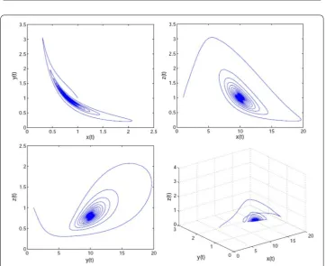
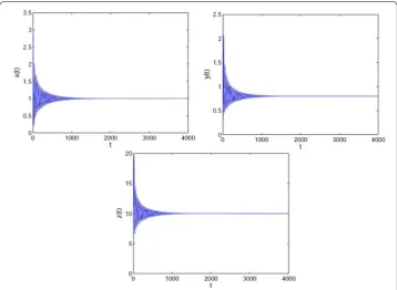
⎧ obtain thatτ0= 6.834. It is known from Theorem1that system (31) is asymptotically stable

at the equilibrium point whenτ∈(0,τ0) (see Figs.1and2), while system (31) produces a

Figure 1The equilibrium (1, 0.8, 10, 10) of system (31) is asymptotically stable whenτ= 6.6 <τ0= 6.834

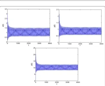
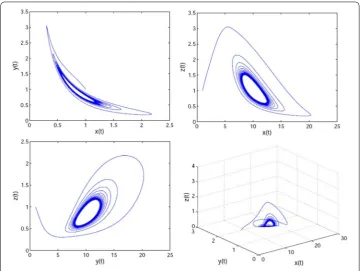
Figure 3A Hopf bifurcation occurs whenτ= 7 >τ0= 6.834, which means that system (31) is unstable

Next, we consider the case of strong kernel. The model is as follows:

⎧ ⎪ ⎪ ⎪ ⎪ ⎪ ⎪ ⎪ ⎪ ⎨ ⎪ ⎪ ⎪ ⎪ ⎪ ⎪ ⎪ ⎪ ⎩

˙

x(t) = –0.2x(t) –y(t)x(t) +_100+v2002, ˙

y(t) = 1 –y(t)x(t) – 0.25y(t), ˙

z(t) = –0.1z(t) +x(t–τ), ˙

u(t) = 1.2z(t) – 1.2u(t), ˙

v(t) = 1.2u(t) – 1.2v(t).

(32)

There is an equilibrium point (x∗,y∗,z∗,u∗,v∗) = (1, 0.8, 10, 10, 10) for system (32). A Hopf bifurcation occurs and a periodic oscillation appears around the equilibrium point whenτ

crosses the critical valueτ0= 6.153 which is calculated by (28). From Theorem2, whenτ ∈

(0,τ0), the equilibrium (x∗,y∗,z∗,u∗,v∗) is stable (see Figs.5and6). Whenτpasses through

an appropriate value, it can cause the loss of stability of equilibrium (x∗,y∗,z∗,u∗,v∗), and system (32) produces an oscillation phenomenon (see Figs.7and8).

Remark3 From the aforementioned simulation, we can clearly observe that the bifurca-tion parameterτ0in system (31) is smaller than that in system (32). This phenomenon

indicates that the system with strong kernel can advance the generation of bifurcation, which means the stable domain of the system can shrink accordingly. Seen from long-term, it may play an important role in analyzing the stability of gene expression processes.

Remark4 It can be found that after the coordinate transformations, the dimension of the gene network with the strong kernel is higher than that of the weak kernel. However, the genetic models with strong kernel or weak kernel are asymptotically stable when the

Figure 6The phase plots of system (32). It is asymptotically stable whenτ= 5.8 <τ0= 6.153

Figure 8The phase plots of system (32). It is unstable whenτ= 6.5 >τ0= 6.153

bifurcation parameters are less than the critical value, and generate limit cycles when the bifurcation parameters are greater than the critical value.

5 Conclusion

We introduce distributed time delays into a gene expression model with sRNA in this paper. Specifically, we take two forms of distributed delays into consideration. The intro-duction of distributed time delay increases the dimension of the network and makes the dynamic behaviors more complex. However, it can describe the time delay of the actual genetic express process more accurately. Here, we take the time delay as the bifurcation parameter to reveal the dynamic behavior of the model. Based on the bifurcation analy-sis of the gene expression model, we obtain that the model is asymptotically stable when the time delay is suitable. Meanwhile, when the delay is greater than the critical value, the model will lose the stability and produce limit cycles.

This paper mainly discusses the effects of distributed delay of the strong kernel and the weak kernel on the stability and periodic oscillation of gene regulatory networks. We con-sider the case where the delay core is 0 and 1. Our future work will be devoted to the dynamical analysis of genetic regulatory networks having a delay core greater than 1. The dimension of the network may increase greatly, which makes the analysis more challeng-ing.

Funding

Competing interests

The authors declare that they have no competing interests.

Authors’ contributions

All authors contributed equally to the writing of this paper. All authors read and approved the final manuscript.

Author details

1_{College of Automation, Nanjing University of Posts and Telecommunications, Nanjing, China.}2_{School of Mathematics} and Physics, Qingdao University of Science and Technology, Qingdao, China. 3_{School of Mathematics and Statistics,} Xinyang Normal University, Xinyang, China.4_{School of Automation and Electrical Engineering, Linyi University, Linyi,} China.5_{College of Science, Nanjing University of Posts and Telecommunications, Nanjing, China.}

Publisher’s Note

Springer Nature remains neutral with regard to jurisdictional claims in published maps and institutional affiliations.

Received: 16 August 2018 Accepted: 6 June 2019

References

1. Liu, L.S., Sun, F.L., Zhang, X.G., Wu, Y.H.: Bifurcation analysis for a singular differential system with two parameters via to degree theory. Nonlinear Anal., Model. Control22(1), 31–50 (2017)

2. Han, M.A., Sheng, L.J., Zhang, X.: Bifurcation theory for finitely smooth planar autonomous differential systems. J. Differ. Equ.264(5), 3596–3618 (2018)

3. Luo, D., Wang, X., Zhu, D., Han, M.: Bifurcation Theory and Methods of Dynamical Systems. World Scientific Publishing, Singapore (1997)

4. Tian, H.H., Han, M.A.: Bifurcation of periodic orbits by perturbing high-dimensional piecewise smooth integrable systems. J. Differ. Equ.263(11), 7448–7474 (2017)

5. Guan, Y.L., Zhao, Z.Q., Lin, X.L.: On the existence of positive solutions and negative solutions of singular fractional differential equations via global bifurcation techniques. Bound. Value Probl.2016, 141 (2016)

6. Romanovski, V.G., Han, M.A., Huang, W.T.: Bifurcation of critical periods of a quintic system. Electron. J. Differ. Equ. 2018(66), 1 (2018)

7. Liu, H.D., Meng, F.W.: Interval oscillation criteria for second-order nonlinear forced differential equations involving variable exponent. Adv. Differ. Equ.2016, 291 (2016)

8. Shao, J., Zheng, Z.W., Meng, F.W.: Oscillation criteria for fractional differential equations with mixed nonlinearities. Adv. Differ. Equ.2013, 323 (2013)

9. Xiao, M., Zheng, W.X., Jiang, G.P.: Bifurcation and oscillatory dynamics of delayed cyclic gene networks including small RNAs. IEEE Trans. Cybern.49(3), 883–896 (2019)

10. Xiao, M., Zheng, W.X., Jiang, G.P., Cao, J.D.: Stability and bifurcation analysis of arbitrarily high-dimensional genetic regulatory networks with hub structure and bidirectional coupling. IEEE Trans. Circuits Syst. I, Regul. Pap.63, 1243–1254 (2016)

11. Huang, C.D., Cao, J.D., Xiao, M.: Hybrid control on bifurcation for a delayed fractional gene regulatory network. Chaos Solitons Fractals87, 19–29 (2016)

12. Xiao, M., Cao, J.D.: Genetic oscillation deduced from Hopf bifurcation in a genetic regulatory network with delays. Math. Biosci.215, 55–63 (2008)

13. Zhang, Y., Liu, H., Yan, F., Zhou, J.: Oscillatory behaviors in genetic regulatory networks mediated by microRNA with time delays and reaction-diffusion terms. IEEE Trans. Nanobiosci.16, 166–176 (2017)

14. Xiao, M., Zheng, W.X., Cao, J.: Stability and bifurcation of genetic regulatory networks with small RNAs and multiple delays. Int. J. Comput. Math.91, 907–927 (2014)

15. Shen, J., Liu, Z., Zheng, W.: Oscillatory dynamics in a simple gene regulatory network mediated by small RNAs. Physica A388, 2995–3000 (2009)

16. Elowitz, M.B., Leibler, S.: A synthetic oscillatory network of transcriptional regulators. Nature403, 335–338 (2000) 17. Chen, L., Aihara, K.: A model of periodic oscillation for genetic regulatory systems. IEEE Trans. Circuits Syst. I, Fundam.

Theory Appl.49, 1429–1436 (2002)

18. Yue, D., Guan, Z.H., Chen, J.: Bifurcations and chaos of a discrete-time model in genetic regulatory networks. Nonlinear Dyn.87, 567–586 (2017)

19. Zhang, X., Han, Y.Y., Wu, L.G., Wang, Y.T.: State estimation for delayed genetic regulatory networks with reaction-diffusion terms. IEEE Trans. Neural Netw. Learn. Syst.29, 299–309 (2018)

20. Ali, M.S., Gunasekaran, N., Ahn, C.K., Shi, P.: Sampled-data stabilization for fuzzy genetic regulatory networks with leakage delays. IEEE/ACM Trans. Comput. Biol. Bioinform.15, 271–285 (2018)

21. Wang, W.Q., Zhong, S.M., Liu, F., Chen, J.: Robust delay-probability-distribution-dependent stability of uncertain stochastic genetic regulatory networks with random discrete delays and distributed delays. Int. J. Robust Nonlinear Control24, 2574–2596 (2014)

22. Llibre, J., Zhang, X.: Darboux theory of integrability in image taking into account the multiplicity. J. Differ. Equ.246, 541–551 (2009)

23. Meng, Q., Jiang, H.J.: Robust stochastic stability analysis of Markovian switching genetic regulatory networks with discrete and distributed delays. Neurocomputing74, 362–368 (2010)

24. Cao, J., Yuan, K., Li, H.X.: Global asymptotical stability of recurrent neural networks with multiple discrete delays and distributed delays. IEEE Trans. Neural Netw.17(6), 1646–1651 (2006)

25. Bi, P., Hu, Z.: Hopf bifurcation and stability for a neural network model with mixed delays. Appl. Math. Comput. 218(12), 6748–6761 (2012)

27. Zhao, H., Wang, L., Ma, C.: Hopf bifurcation and stability analysis on discrete-time Hopfield neural network with delay. Nonlinear Anal.9(1), 103–113 (2008)

28. Liao, X., Chen, G.: Hopf bifurcation and chaos analysis of Chen’s system with distributed delays. Chaos Solitons Fractals25(1), 197–220 (2005)

29. Xu, W., Cao, J., Xiao, M.: A new framework for analysis on stability and bifurcation in a class of neural networks with discrete and distributed delays. IEEE Trans. Cybern.45, 2224–2236 (2015)

30. Xu, C.J., Shao, Y.F.: Bifurcations in a predator-prey model with discrete and distributed time delay. Nonlinear Dyn.67, 2207–2223 (2012)

31. Xiao, M., Zheng, W.X., Cao, J.: Frequency domain approach to computational analysis of bifurcation and periodic solution in a two-neuron network model with distributed delays and self-feedbacks. Neurocomputing99, 206–213 (2013)

32. Niu, B., Guo, Y.X.: Bifurcation analysis on the globally coupled Kuramoto oscillators with distributed time delays. Physica D266, 23–33 (2014)

33. Mu, Y., Li, Z.X., Xiang, H.L., Wang, H.L.: Bifurcation analysis of a turbidostat model with distributed delay. Nonlinear Dyn.90, 1315–1334 (2017)

34. Elaiw, A.W., AlShamrani, N.H.: Stability of a general delay-distributed virus dynamics model with multi-staged infected progression and immune response. Math. Methods Appl. Sci.40, 699–719 (2017)

35. Ling, G., Guan, Z.H., Liao, R.Q., Cheng, X.M.: Stability and bifurcation analysis of cyclic genetic regulatory networks with mixed time delays. SIAM J. Appl. Dyn. Syst.14, 202–220 (2015)