Multiple soliton solutions for the variant Boussinesq equations

R E S E A R C H

Open Access

Multiple soliton solutions for the variant

Boussinesq equations

Peng Guo

_{, Xiang Wu}

_{and Liang-bi Wang}

*_{Correspondence:} [email protected] 1_{School of Mathematics and} Physics, Lanzhou Jiaotong University, Lanzhou, 730070, P.R. China

2_{School of Mechatronic} Engineering, Lanzhou Jiaotong University, Lanzhou, 730070, P.R. China

Full list of author information is available at the end of the article

Abstract

The Hirota bilinear method is used to handle the variant Boussinesq equations. Multiple soliton solutions and multiple singular soliton solutions are formally established. It is shown that the Hirota bilinear method may provide us with a straightforward and effective mathematic tool for generating multiple soliton solutions of nonlinear wave equations in fluid mechanics.

Keywords: Hirota bilinear method; the variant Boussinesq equations; multiple soliton solutions; multiple singular soliton solutions

1 Introduction

Many phenomena in physics, biology, chemistry, mechanics,etc.are described by non-linear partial differential equations. Nonnon-linear wave phenomena of dissipation, diffusion, reaction, and convection are very important, and they can be represented with a variety of nonlinear wave equations. The investigation of exact solutions of these equations will help ones to understand these phenomena better.

During the past several decades, many powerful and efficient methods have been pro-posed to obtain the exact solutions of nonlinear wave equations, such as inverse scattering method [], Darboux and Bäcklund transformations [, ], the Hirota bilinear method [], the tanh method [], the extended tanh method [], the sine-cosine method [], the homo-geneous balance method [], the homotopy perturbation method [, ], theF-expansion method [], the Exp-function expansion method [, ], the (G/G)-expansion method [, ], the Kudryashov method [], the mapping method [], the extended mapping method [], and so on.

The above methods can be used to handle the nonlinear wave equations for single soliton solutions, but the multiple soliton solutions of the nonlinear wave equations can be ob-tained only by three different methods: the inverse scattering method, the Bäcklund trans-formation method, and the Hirota bilinear method. However, the Hirota bilinear method is rather heuristic and possesses significant features that make it be ideal for the deter-mination of multiple soliton solutions for a wide class of the nonlinear wave equations [–]. When the Hirota bilinear method is used, computer symbolic systems such as Maple and Mathematica allow us to perform complicated and tedious calculations.

The Boussinesq equation is a well-known model of long water wave of moderate am-plitude, describes one dimensional, weakly nonlinear internal wave which develops at the boundary between two immiscible fluids. In addition, the equation is a simplified

model of the atmospheric movement equation which is applicable to mesoscale and quasi-incompressible fluid movement, which means important physical applications in hydro-dynamics. The Boussinesq equation also is of considerable mathematic interests because of its rich mathematical structures. In the present research, we focus on the variant Boussi-nesq equations, which was derived by Sachs [] in  as a model for water waves:

Ht+ (Hu)x+uxxx= ,

ut+Hx+uux= ,

()

whereu(x,t) is the velocity,H(x,t) is the height of free wave surface for fluid in the trough, and the subscripts denote partial derivatives. In the past years, many authors have studied Eq. (). For example, Wang [] solved Eq. () by the homogeneous balance method. Yan and Zhang [] obtained new explicit and exact traveling wave solutions for Eq. () by an improved sine-cosine method and the Wu elimination method. Nazet al.[] obtained the conservation laws for Eq. () by an interesting method of increasing the order of partial differential equations. Fan and Hon [] uniformly constructed a series of traveling wave solutions for Eq. () by a new algebraic method. Lü [] solved Eq. () by a general Jacobi elliptic function expansion method, and obtained Jacobi elliptic function solutions. Yuan

et al.[] constructed bifurcations of traveling wave solutions for Eq. () by the bifurcation theory of planar dynamical systems. Liet al.[] obtained all possible smooth, cusped solitary wave solutions for Eq. () by the phase portrait analytical technique.

The above review shows that many works to obtain the exact solutions of Eq. () have been carried out in recent years, but the multiple soliton solutions for Eq. () have not been obtained. The existence of multiple soliton solutions often implies the integrability of the considered equations. The objectives of this paper are twofold. First, we aim to apply the Hirota bilinear method to handle Eq. (). Second, we seek to establish multiple soli-ton solutions and multiple singular solisoli-ton solutions to confirm that Eq. () is completely integrable. The rest of this paper is organized as follows. In Section , the Hirota bilinear method for finding the multiple soliton solutions of the nonlinear wave equations is de-scribed. In Sections  and , the method to solve Eq. () is illustrated in detail. Multiple soliton solutions and multiple singular soliton solutions are obtained. In Section , some conclusions are given.

2 The Hirota bilinear method

The Hirota direct method is well known, and it gives soliton solutions by polynomials of exponentials. We only summarize the main steps as follows.

(i) Substituting

u(x,t) =eθi_{, θ}

i=kix–cit, ()

into the linear terms of the equation under discussion to determine the dispersion relation betweenkiandci.

(ii) Substituting the single soliton solution

u(x,t) =Rlnf(x,t)_x=Rfx

u(x,t) =Rlnf(x,t)_xx=Rffxx–f



x

f , ()

or

u(x,t) =R

arctan

f(x,t)

g(x,t)

x

=Rfxg–fgx

f_+g ()

into the equation under discussion to determineR, where

f(x,t) =  +eθ_{. ()}

(iii) For a single soliton, we use

f(x,t) =  +eθ_{. ()}

(iv) For two soliton solutions, we use

f(x,t) =  +eθ_+eθ_+a

eθ+θ. ()

(v) For three soliton solutions, we use

f(x,t) =  +eθ_+eθ_+eθ_+a

eθ+θ+aeθ+θ+aeθ+θ+aeθ+θ+θ. ()

If the obtained result shows thata=aaa, then the equation gives multiple soliton solutions and the equation is integrable.

However, for multiple singular soliton solutions, we apply the following steps: (i) For the dispersion relation, we use

u(x,t) =eθi_{, θ}

i=kix–cit. ()

(ii) Next we substitute the single soliton solution

u(x,t) =Rlnf(x,t)_x=Rfx

f , ()

u(x,t) =Rlnf(x,t)_xx=Rffxx–f



x

f , ()

or

u(x,t) =R

arctan

f(x,t)

g(x,t)

x

=Rfxg–fgx

f_+g ()

into the equation under discussion to determineR, where

f(x,t) =  –eθ_{. ()}

(iii) For a single soliton, we use

(iv) For two soliton solutions, we use

f(x,t) =  –eθ_–eθ_+a

eθ+θ. ()

(v) For three soliton solutions, we use

f(x,t) =  –eθ_–eθ_–eθ_+a

eθ+θ+aeθ+θ+aeθ+θ–aeθ+θ+θ. ()

Other approaches will also be used for the multiple singular soliton solutions, as will be examined later.

3 Multiple soliton solutions of the variant Boussinesq equations Substituting the following equations:

H(x,t) =Aekix–cit_,

u(x,t) =Bekix–cit_, ()

into the linear terms of Eq. (), we obtain the dispersion relation

ci=±ki, ()

and as a result we have

θi=kix∓kit, ()

whereAandBare constants. Using the Cole-Hopf transformation method, we assume that the multiple solutions of Eq. () are

H(x,t) =R[lnf(x,t)]xx=Rffxx–f

 x

f , u(x,t) =R[lnf(x,t)]x=Rf_fx,

()

wheref(x,t), for the single soliton solution, is given by

f(x,t) =  +eθ_{=  +e}kx∓kt_{. ()}

Substituting Eq. () into Eq. (), using the result from Eq. (), and solving it forRandR, we find

R=R= . ()

Substituting Eqs. ()-() into Eq. () we obtain the single soliton solution

⎧ ⎪ ⎨ ⎪ ⎩

H(x,t) = k

 e

kx+k_t

(ekt+ekx₎, u(x,t) =kekx–kt

+ekx–kt,

Figure 1 Plots of the solution described by Eq. (24). (a)The single soliton solutionH(x,t) fork1= 0.4.

Figure  shows the single soliton solution for Eq. () for some special values of the solution’s parameters in Eq. ().

For two soliton solutions, we set

f(x,t) =  +eθ_+eθ_+a

eθ+θ=  +ekx∓k



t_+ekx∓kt_+ae(k+k)x∓(k+k)t_{. ()}

Using Eqs. () and () into Eq. () and substituting the result into Eq. (), we obtain the phase shift by

a= , ()

and hence we set

aij= , ≤i<j≤N. ()

The two soliton solutions are obtained by substituting Eqs. () and () into Eq. (),

⎧

Figure  shows the two soliton solutions for Eq. () for some special values of the solution’s parameters in Eq. ().

For three soliton solutions, we set

Figure 2 Plots of the solution described by Eq. (29). (a)The two soliton solutionsH(x,t) fork1= 0.4,

k2= 0.8.(b)The two soliton solutionsu(x,t) fork1= 0.4,k2= 0.8.

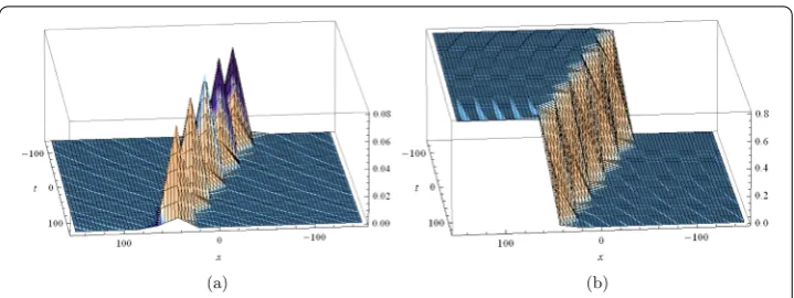
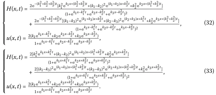
Figure 3 Plots of the solution described by Eq. (32). (a)The three soliton solutionsH(x,t) fork1= 0.4,

k2= 0.8,k3= 1.55.(b)The three soliton solutionsu(x,t) fork1= 0.4,k2= 0.8,k3= 1.45.

Proceeding as before, we find that the three soliton solutions are given by

⎧ ⎪ ⎪ ⎪ ⎪ ⎪ ⎪ ⎨ ⎪ ⎪ ⎪ ⎪ ⎪ ⎪ ⎩

H(x,t) = e

–(k_{ +} k_{ +} k_{ )}t

[k_ekx+(k +k )t+(k–k)e(k+k)x+kt+k_ekx+(k +k )t] (+ekx–kt+ekx–kt+ekx–kt)

+e

–(k_{ +}k_{ +}k_{ )}t

[(k–k)e(k+k)x+kt+(k–k)e(k+k)x+kt+k_ekx+(k + k )t] (+ekx–kt+ekx–kt+ekx–kt) , u(x,t) =(kekx–kt+kekx–kt+kekx–kt)

+ekx–kt₊ekx–kt₊ekx–kt ,

()

⎧ ⎪ ⎪ ⎪ ⎪ ⎪ ⎪ ⎨ ⎪ ⎪ ⎪ ⎪ ⎪ ⎪ ⎩

H(x,t) = [ke kx+k_t

+(k–k)e(k+k)x+(k + k )t+k_ekx+kt] (+ekx+kt+ekx+kt+ekx+k

 t)

+[(k–k)

_e(k+k)x+(k_{ +} k_{ )}t

+(k–k)e(k+k)x+(k + k )t+k_ekx+kt] (+ekx+kt+ekx+kt+ekx+kt) , u(x,t) =(kekx+kt+kekx+kt+kekx+kt)

+ekx+kt+ekx+kt+ekx+kt .

()

Figure  shows the three soliton solutions for Eq. () for some special values of the solu-tion’s parameters in Eq. ().

solutions can be set as

4 Multiple singular soliton solutions of the variant Boussinesq equations Substituting

H(x,t) =Aekix–cit_,

u(x,t) =Bekix–cit_, ()

into the linear terms of Eq. () to find that the dispersion relation is

ci=±ki, ()

and as a result we obtain

θi=kix∓kit, ()

whereAandBare constants. Using the Cole-Hopf transformation method, the multiple singular soliton solutions of Eq. () are assumed to be

wheref(x,t), for the single singular soliton solution, is given by

f(x,t) =  –eθ_{=  –e}kx∓kt_{. ()}

Substituting Eq. () into Eq. () and solving forRandRwe find

R=R= . ()

This means that the single singular soliton solution is given by

Figure 4 Plots of the solution described by Eq. (42). (a)The single singular soliton solutionH(x,t) for

k1= 0.4.(b)The single singular soliton solutionu(x,t) fork1= 0.4.

Figure  shows the single singular soliton solution for Eq. () for some special values of the solution’s parameters in Eq. ().

For two singular soliton solutions, we set

f(x,t) =  –eθ_–eθ_+a

eθ+θ=  –ekx∓k



t_–ekx∓kt_+ae(k+k)x∓(k+k)t_{. ()}

Using Eq. () into Eq. () and substituting the result into Eq. (), we obtain the phase shift

a= , ()

and hence we set

aij= , ≤i<j≤N. ()

The two singular soliton solutions are obtained by substituting Eqs. () and () into Eq. (), where we find

⎧ ⎪ ⎨ ⎪ ⎩

H(x,t) = –e

(k_{ +}k_{ )}t

[k_ekx+kt–(k–k)e(k+k)x+k_ekx+kt] (–e(k



 +k )t+ekx+k  t+ekx+k



t) , u(x,t) =(–kekx–k

 t–kekx–k

 t) –ekx–k

 t–ekx–k

 t

,

()

⎧ ⎪ ⎨ ⎪ ⎩

H(x,t) = –ke k_x+k_t

–ekx+kt_{[(k–k)}_ek_x+k_t

+k]

(–+ekx+kt₊ekx+kt₎ , u(x,t) = –(kekx+kt+kekx+kt)

–ekx+kt_–ekx+kt .

()

Figure  shows the two singular soliton solutions for Eq. () for some special values of the solution’s parameters in Eq. ().

For three singular soliton solutions, we set

Figure 5 Plots of the solution described by Eq. (47). (a)The two singular soliton solutionsH(x,t) for

k1= 0.4,k2= 0.8.(b)The two singular soliton solutionsu(x,t) fork1= 0.4,k2= 0.8.

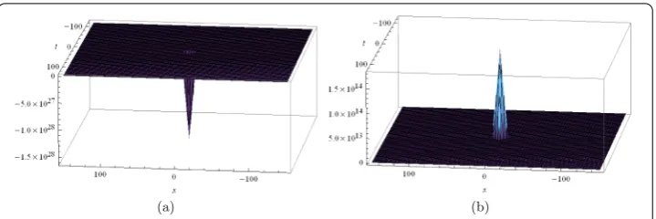
Figure 6 Plots of the solution described by Eq. (50). (a)The three singular soliton solutionsH(x,t) for

k1= 0.4,k2= 0.8,k3= 1.55.(b)The three singular soliton solutionsu(x,t) fork1= 0.4,k2= 0.8,k3= 1.45.

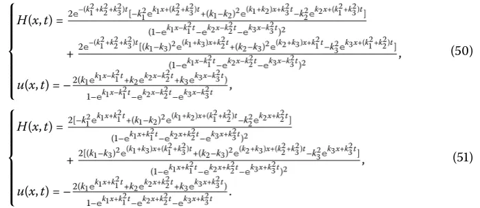
Proceeding as before, we find the following three singular soliton solutions: ⎧

Figure  shows the three singular soliton solutions for Eq. () for some special values of the solution’s parameters in Eq. ().

⎧

The Hirota bilinear method is applied to emphasize the integrability of the variant Boussi-nesq equations. Multiple soliton solutions and multiple singular soliton solutions are for-mally derived. The analysis confirms the fact that the variant Boussinesq equations have

Nsoliton solutions, and haveNsingular soliton solutions simultaneously. The results ob-tained for the phase shiftaijshow that the system is resonance free. The method used here

is standard and direct, so we believe that multiple soliton solutions and multiple singular soliton solutions may exist for other classes of nonlinear mathematic physics models, such as the coupled Kadomtsev-Petviashvili system, the Davey-Stewartson system, the gener-alized Hirota-Satsuma coupled KdV system, and so on. Further work on these aspects is worthy of performing.

Competing interests

The authors declare that they have no competing interests.

Authors’ contributions

The authors have equal contributions to each part of this paper. All the authors read and approved the final manuscript.

Author details

1_{School of Mathematics and Physics, Lanzhou Jiaotong University, Lanzhou, 730070, P.R. China.}2_{School of Mechatronic} Engineering, Lanzhou Jiaotong University, Lanzhou, 730070, P.R. China.3_{Key Laboratory of Railway Vehicle Thermal} Engineering, Lanzhou Jiaotong University, Ministry of Education, Lanzhou, 730070, P.R. China.

Acknowledgements

The authors would like to express their sincere thanks to editors and referees for their valuable suggestions and comments. This work was supported by the National Natural Science Foundation of China under Grant no. 11464027, the Scientific Research Foundation of the Higher Education Institutions of Gansu Province under Grant no. 2014A-053, and the Young Scholars Science Foundation of Lanzhou Jiaotong University under Grant no. 2013026.

Received: 28 September 2014 Accepted: 13 January 2015

References

1. Ablowitz, MJ, Clarkson, PA: Soliton, Nonlinear Evolution Equations and Inverse Scattering. Cambridge Universty Press, New York (1991)

2. Matveev, VB, Salle, MA: Darboux Transformation and Solitons. Springer, Berlin (1991) 3. Miura, MR: Backlund Transformation. Springer, Berlin (1978)

4. Hirota, R: Exact solution of the Korteweg-de Vries equation for multiple collisions of solitons. Phys. Rev. Lett.27, 1192-1194 (1971)

5. Parkes, EJ, Duffy, BR: An automated tanh-function method for finding solitary wave solutions to non-linear evolution equations. Comput. Phys. Commun.98, 288-300 (1996)

6. Fan, EG: Extended tanh-function method and its applications to nonlinear equations. Phys. Lett. A277, 212-218 (2000)

7. Yan, CT: A simple transformation for nonlinear waves. Phys. Lett. A224, 77-84 (1996)

8. Wang, ML: Exact solutions for a compound KdV-Burgers equation. Phys. Lett. A213, 279-287 (1996) 9. Chun, C, Sakthivel, R: Homotopy perturbation technique for solving two-point boundary value

problems-comparison with other methods. Comput. Phys. Commun.181, 1021-1024 (2010)

10. Sakthivel, R, Chun, C, Lee, J: New travelling wave solutions of Burgers equation with finite transport memory. Z. Naturforsch. A65, 633-640 (2010)

11. Abdou, MA: The extendedF-expansion method and its application for a class of nonlinear evolution equations. Chaos Solitons Fractals31, 95-104 (2007)

12. He, JH: Exp-function method for nonlinear wave equations. Chaos Solitons Fractals30, 700-708 (2006) 13. Sakthivel, R, Chun, C: New soliton solutions of Chaffee-Infante equations using the Exp-function method.

Z. Naturforsch. A65, 197-202 (2010)

14. Zayed, EME, Gepreel, KA: The (G/G)-expansion method for finding traveling wave solutions of nonlinear partial differential equations in mathematical physics. J. Math. Phys.50, 013502 (2009)

16. Kim, H, Bae, JH, Sakthivel, R: Exact travelling wave solutions of two important nonlinear partial differential equations. Z. Naturforsch. A69, 155-162 (2014)

17. Lou, SY, Ni, GJ: The relations among a special type of solitons in some (D+ 1) dimensional nonlinear equations. J. Math. Phys.30, 1614-1620 (1989)

18. Bai, CJ, Zhao, H, Xu, HY, Zhang, X: New traveling wave solutions for a class of nonlinear evolution equations. Int. J. Mod. Phys. B25, 319-327 (2011)

19. Hirota, R, Ito, M: Resonance of solitons in one dimension. J. Phys. Soc. Jpn.52, 744-748 (1983) 20. Hirota, R: The Direct Method in Soliton Theory. Cambridge University Press, Cambridge (2004)

21. Hirota, R: Exact solutions of the modified Korteweg-de Vries equation for multiple collisions of solitons. J. Phys. Soc. Jpn.33, 1456-1458 (1972)

22. Hirota, R: Exact solutions of the Sine-Gordon equation for multiple collisions of solitons. J. Phys. Soc. Jpn.33, 1459-1463 (1972)

23. Hietarinta, J: A search for bilinear equations passing Hirota’s three-soliton condition. I. KdV-type bilinear equations. J. Math. Phys.28, 1732-1742 (1987)

24. Hietarinta, J: A search for bilinear equations passing Hirota’s three-soliton condition. II. mKdV-type bilinear equations. J. Math. Phys.28, 2094-2101 (1987)

25. Wazwaz, AM: Partial Differential Equations and Solitary Waves Theory. Higher Education Press, Beijing (2009) 26. Sachs, RL: On the integrable variant of the Boussinesq system: Painlevé property, rational solutions, a related

many-body system, and equivalence with the AKNS hierarchy. Physica D30, 1-27 (1988)

27. Wang, ML: Solitary wave solutions for variant Boussinesq equations. Phys. Lett. A199, 169-172 (1995)

28. Yan, ZY, Zhang, HQ: New explicit and exact travelling wave solutions for a system of variant Boussinesq equations in mathematical physics. Phys. Lett. A252, 291-296 (1999)

29. Naz, R, Mahomed, FM, Hayat, T: Conservation laws for third-order variant Boussinesq system. Appl. Math. Lett.23, 883-886 (2010)

30. Fan, EG, Hon, YC: A series of travelling wave solutions for two variant Boussinesq equations in shallow water waves. Chaos Solitons Fractals15, 559-566 (2003)

31. Lü, DZ: Jacobi elliptic function solutions for two variant Boussinesq equations. Chaos Solitons Fractals24, 1373-1385 (2005)

32. Yuan, YB, Pu, DM, Li, SM: Bifurcations of travelling wave solutions in variant Boussinesq equations. Appl. Math. Mech.

27, 811-822 (2006)