R E S E A R C H
Open Access
The eigenvalues and sign-changing
solutions of a fractional boundary value
problem
Xiangkui Zhao
*and Fengjiao An
*Correspondence: [email protected] Department of Applied Mathematics, School of
Mathematics and Physics, University of Science and Technology Beijing, Beijing, 100083, P.R. China
Abstract
In this paper, we are interested in the eigenvalues and its algebraic multiplicities of a fractional linear boundary value problem with mixed set of Neumann and Dirichlet boundary conditions. The research results are then applied to consider the
sign-changing solutions of the corresponding nonlinear problem by fixed point index and Leray-Schauder degree. To date, no paper has appeared in the literature which discusses sign-changing solutions of fractional boundary value problems. This paper attempts to fill this gap in the literature.
MSC: 26A33; 34A08; 34B09
Keywords: eigenvalues; fractional differential equations; sign-changing solutions; fixed point index; Leray-Schauder degree
1 Introduction
With the development of science and technology, researchers have paid much attention to the fractional differential equations, it is extensively applied in various sciences, such as physics, mechanics, chemistry, engineering, astronomy,etc. There are a lot of research papers about the fractional differential equation boundary value problems; see [–] and the references therein. Most of them are devoted to the existence and multiplicity of pos-itive solutions; see [, , –]. For example, in [], the author considered the existence of positive solutions for a class of nonlinear boundary value problems of Caputo fractional equations with integral boundary conditions,
⎧ ⎨ ⎩
cDα
ty(t) +f(y(t)) = , <t< , y() =y() = , y() =λy(s)ds.
In [], the author considered the existence and multiplicity of positive solutions for a non-linear boundary value problem involving Caputo’s derivative
⎧ ⎨ ⎩
cDα
ty(t) =f(t,y(t)), t∈(, ), y() +y() = , y() +y() = .
To the best of the author’s knowledge, although sign-changing solutions of integer bound-ary value problems with different conditions are extensively studied by computing the al-gebraic multiplicities of eigenvalues, see for example [–] and the references therein, to date, no paper has appeared in the literature which discusses sign-changing solutions of fractional boundary value problems due to the intrinsic distinction between the eigen-values of fractional problems and the integer problems. For example, the eigeneigen-values of fractional differential equations have no periodicity.
Motivated by the above papers, first, we investigate the following eigenvalue problem with the mixed set of Neumann and Dirichlet boundary conditions,
⎧ ⎨ ⎩
cDα
tu(t) +λu(t) = , t∈(, ),
u() = , u() = . (.)
Then we establish some existence results of sign-changing solutions for the following non-linear fractional boundary value problem with the same boundary conditions:
⎧ ⎨ ⎩
cDα
tu(t) +f(u(t)) = , t∈(, ),
u() = , u() = , (.)
where <α< is a real number andcDα
t is the Caputo fractional derivative,f :R→R.
For convenience in the presentation, throughout this paper, let
β=lim
x→
f(x)
x , β∞=xlim→∞
f(x)
x .
And we always assume the following conditions are satisfied:
(H) f(x)∈C(R,R),f(θ) =θ,xf(x) > for allx∈R\ {θ}.
(H) There exist two positive integersnandn. Andn,nmay be equal, with
λn<β<λn+, λn<β∞<λn+,
where <λ<λ<· · ·<λnα are the eigenvalues of (.),nαis the number of
eigenvalues.
(H) There exists a positive constant numberC> such that|f(x)|<(α)Cfor allx
with|x| ≤C.
We shall organize the rest of this paper as follows. In Section , some basic definitions and preliminaries are given. Furthermore the eigenvalues and its algebraic multiplicities of (.) are considered. In Section , the sign-changing solutions of (.) are considered. An example will be given to illustrate the application in Section .
2 Some basic definitions and preliminaries
Definition . The Caputo fractional derivative of order α > for the function y: (, +∞)→Ris defined as
cDα
ty(t) =
(m–α) t
y(m)(s)
(t–s)α–m+ds,
Definition . The Riemann-Liouville fractional integral of orderαfor the functionf is defined as
I+α f(t) =
(α) t
(t–s)α–f(s)ds, α> ,
provided that the right side is point-wise defined on (,∞).
Definition . The Mittag-Leffler function with two parameters is defined by the series expansion
Eα,β(z) =
∞
k=
zk
(αk+β), α> ,β> ,z∈C,
which is analytic on the whole complex plane.
Now we investigate the eigenvalue problem (.). From the Laplace transform of the Caputo fractional derivative []
LcDα
tu(t) =s
αL
u(t) –
m–
i=
sα–i–u(i)(), m– <α≤m,
andu() = , we have
LcDα
tu(t) +λu(t) =s
αL
u(t) –sα–u() +λLu(t) = .
Hence
Lu(t) =u() s α–
sα+λ.
From the inverse Laplace transform of the Mittag-Leffler function []
Eα,
–λtα=L–
sα–
sα+λ
,
we get
u(t) =u()Eα,
–λtα.
Byu() = , we know
Eα,(–λ) = .
Henceλis the eigenvalue of (.) if and only ifλis a solution ofEα,(–x) = , and for all
nonzero constantsC∈R,u(t) =CEα,(–λtα) are the eigenfunctions corresponding
Then we consider the inverse problem of (.). It follows from the definition of the Ca-puto fractional derivative thatuis an eigenfunction of (.) corresponding to the eigen-valueλ, if and only ifuis a solution of the integral equation
u(t) =
λG(t,s)u(s)ds, (.)
where
G(t,s) = ⎧ ⎨ ⎩
(–s)α––(t–s)α–
(α) , ≤s≤t≤, (–s)α–
(α) , ≤t≤s≤.
(.)
Define the operatorT as follows:
(Tu)(t) = t
( –s)α–– (t–s)α–
(α) u(s)ds+
t
( –s)α–
(α) u(s)ds.
Therefore, we know thatλ= is an eigenvalue of (.) if and only if λ is an eigenvalue of operatorT. That is,
λ is an eigenvalue of operatorT if and only ifλis a solution of
Eα,(–x) = . Andu(t) =CEα,(–λtα) (C= ) are the eigenfunctions corresponding to the
eigenvalue λ. Let
λ<λ<· · ·<λnα
be the sequence of solutions to the equationEα,(–x) = . From [], we see thatλj(j=
, , . . . ,nα) are positive andnαis finite. By computing, we can get
n.=n.=n.=n.= , n.= , n.= , n.= , . . . .
That is, whenα= ., ., ., ., the operatorT has one eigenvalue, whenα= .,Thas three eigenvalues, whenα= .,T has five eigenvalues, whenα= .,T has nine eigen-values, and so on. Furthermore we will consider the algebraic multiplicity of λ.
Lemma . Assume
λ is the eigenvalue of T, that is, Eα,(–λ) = . Furthermore
E()α,(–λ)= .Then the algebraic multiplicity of eigenvalueλfor T is equal to.
Proof It is obvious that
ker(I–λT)⊆ker(I–λT).
Letu∈ker(I–λT), ifu∈/ker(I–λT), then there exists a nonzero constantCsuch that
(I–λT)u(t) =CEα,
sinceCEα,(–λtα) (C= ) are the eigenfunctions of operatorTcorresponding to the
eigen-value λ. By direct computation, we have ⎧
From the Laplace transform of the Caputo fractional derivative [],
LDαu(t) =sαLu(t) –
m–
i=
sα–i–u(i)(), m– <α≤m,
the Laplace transform of the Mittag-Leffler function [],
Ltμ–Eα,μ
From the inverse Laplace transform of the Mittag-Leffler function [],
we see that the algebraic multiplicity of the eigenvalueλ is equal to . This completes the Then we need to show
ker(I–λT)⊆ker(I–λT).
By direct computation, we have ⎧
From the Laplace transform of the Caputo fractional derivative, the Laplace transform of the Mittag-Leffler function [, ] andu() = , we have
From the inverse Laplace transform of the Mittag-Leffler function [], we can obtain
Letu() = , then we get
E()α,(–λ) = ,
which is a contradiction. Hence
ker(I–λT)⊆ker(I–λT).
Therefore
ker(I–λT)=ker(I–λT).
That is, the algebraic multiplicity of the eigenvalue λ is equal to . This completes the
proof.
Similarly to Lemma ., Lemma ., we can study the algebraic multiplicity of eigenvalue
λ for operatorTby Laplace transforms. Then we will consider the sign-changing solutions of (.) by the algebraic multiplicity of the eigenvalue λfor the operatorT.
3 The existence of sign-changing solutions Consider the Banach space
E=u∈C[, ] :u() = ,u() =
with the normu=max{u∞,u∞}, whereu∞=max≤t≤|u(t)|. Let
P=u∈E:u(t)≥,∀t∈[, ]
be a cone ofE. Define operatorsFandBas follows:
(Fu)(t) =fu(t), t∈(, ),u∈E
and
B=T◦F.
Thenuis a solution of (.) if and only ifuis a solution of the operator equation
u=Bu.
By (H), we can see thatB,Tare completely continuous.
Lemma . Assume that(H)hold,then the operator B is Fréchet differentiable atθand
Proof Fromβ=limx→f(xx), we have∀ε> ,∃δ> ,∀ <|x|<δ, and we see that
Similarly, we can show that
Similarly, we can show that
(Bu–β∞Tu)∞<
(α)
εu+M, u∈E.
Hence
Bu–β∞Tu<
(α)
εu+M.
Consequently
lim u→∞
Bu–β∞Tu
u = . (.)
ThereforeBis Fréchet differentiable at∞, andB(∞) =β∞T.
Lemma . Assume that(H)hold,u∈P\ {θ}is a solution of(.),then u∈P˚.
Proof Ifu∈P\ {θ}is a solution of (.), then
u(t) =
G(t,s)fu(s)ds
= t
( –s)α–– (t–s)α–
(α) f
u(s)ds+
t
( –s)α–
(α) f
u(s)ds,
u(t) = –
(α) t
(α– )(t–s)α–fu(s)ds.
It is obvious that
u() = , u() = , u() > , u() < , u(t) < .
Fromu() < we learn that there existε> ,τ> , such that
u(t) < –τ, ∀t∈[ –ε, ]. (.)
Fromu() = ,u(t) < ,∀t∈(, ] we learn that there existsτ> , such that
u(t) >τ, ∀t∈[, –ε]. (.)
Letτ=min(τ,τ), then ifx–u<τfor anyx∈E, we can getx(t)≥,t∈[, ] by (.),
(.), that is,x∈P. ConsequentlyB(u,τ)⊂Pandu∈P˚.
Lemma .([]) Let P be a solid cone of real Banach space E,be a relatively bounded open set of P,A:P→P be a completely continuous operator.If all fixed points of A are an interior point of P,there exists an open subset O of E such that O⊂anddeg(I–A,O,θ) =
i(A,,P).
problem(.)has at least two sign-changing solutions,two positive solutions and two neg-ative solutions.
Proof It follows from the definition ofBthatuis a solution of (.) if and only ifuis the fixed point of the operatorB. Then by (H), we have, for anyu∈Ewithu=C,
by Theorem ., in [], we know that there exist a small enoughrand a large enough
Rsuch that
wherekis the sum of the algebraic multiplicities of the real eigenvalues ofB(θ) which are
larger than ,kis the sum of the algebraic multiplicities of the real eigenvalues ofB(∞)
which are larger than .
Hence, by (.), (.), (.), we see that
Therefore the operatorBhas at least two fixed points
u∈P∩
That is,u andu are positive solutions of the boundary value problem (.) and r <
Similarly we can see that
degI–B,U(θ,R),θ
= (–)k= (–)n= . (.)
From (.), (.), (.), and (.) we see that
degI–B,U(θ,C)\
O∪O∪U(θ,r)
,θ= – – – = –. (.)
By (.), we knowBhas at least one fixed pointu∈U(θ,C)\(O∪O∪U(θ,r)).
That is, boundary value problem (.) has a sign-changing solutionu. Similarly, we get
another different solutionu∈U(θ,C)\(O∪O∪U(θ,C)) by (.), (.), (.), and
(.). This completes the proof.
According to the method used in the proof of Theorem ., we can give the following corollaries.
Corollary . Let(H)-(H)hold, <λ<λ<· · ·<λnα are the eigenvalues of(.),there
exists a positive integer nsuch thatλn<β<λn+orλn<β∞<λn+and E
()
α,(–λj)=
,where j= , , . . . , n.Then the boundary value problem(.)have at least one
sign-changing solution,one positive solution and one negative solution.
Corollary . Let(H)-(H)hold,λis the eigenvalue of(.),E()α,(–λ)= .
() Ifβ∞<λ<βorβ<λ<β∞,then the boundary value problem(.)has at least
one positive solution and one negative solution.
() Ifβ>λ,β∞>λ,then the boundary value problem(.)has at least two positive
solutions and two negative solutions.
4 Example
Consider the following fractional differential equation:
⎧ ⎨ ⎩
cD.
x u(t) +f(u(t)) = , t∈(, ),
u() = , u() = , (.)
where
f(u) = ⎧ ⎪ ⎪ ⎨ ⎪ ⎪ ⎩
–, u≤–, u, – <u< ,
,
≤u.
(.)
We can find that
() β=limu→f(uu) = ;
() f(u) :R→R,f(θ) =θ,uf(u) > for allt∈(, ),u∈R\ {θ};
() from [, ], we see thatE.,(–x) = has three zero points,x= .,x= .,
x= ., andEα(),(–x)= ,E()α,(–x)= ;
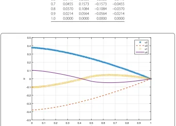
Table 1 Sign-changing solutionsu1,u4, positive solutionu2, negative solutionu3
t u1 u2 u3 u4
0.0 –0.1025 0.3772 –0.3772 0.1025 0.1 –0.0910 0.3657 –0.3657 0.0910 0.2 –0.0692 0.3439 –0.3439 0.0692 0.3 –0.0411 0.3158 –0.3158 0.0411 0.4 –0.0077 0.2824 –0.2824 0.0077 0.5 0.0293 0.2446 –0.2446 –0.0293 0.6 0.0449 0.2028 –0.2028 –0.0449 0.7 0.0455 0.1573 –0.1573 –0.0455 0.8 0.0370 0.1084 –0.1084 –0.0370 0.9 0.0214 0.0564 –0.0564 –0.0214 1.0 0.0000 0.0000 0.0000 0.0000
Figure 1 Sign-changing solutionsu1,u4, positive solutionu2, negative solutionu3.
() letC= , when– <u<, we have
f(u)=|u| ≤
<(.)
whenu≤– or ≤u, we have
f(u)=
<(.).
By Corollary ., we see that problem (.) has at least one sign-changing solution
u, one positive solutionu, one negative solutionu. Byf(–u) = –f(u), we see that
u= –uis another sign-changing solution of (.). The numerical results ofu,u,
uanduare shown in Table , the graphs ofu,u,uanduare shown in Figure .
5 Conclusion
their algebraic multiplicities are established. Finally, an example is presented to illustrate the application.
Competing interests
The authors declare that they have no competing interests.
Authors’ contributions
XZ raised these interesting problems. All authors contributed to the proofs of the main results and approved the final version of the manuscript.
Acknowledgements
The authors thank for the editors and referees for valuable comments. This work was supported by the Fundamental Research Funds for the Central Universities.
Received: 11 March 2016 Accepted: 11 April 2016
References
1. Cabada, A, Wang, GT: Positive solutions of nonlinear fractional differential equations with integral boundary value conditions. J. Math. Anal. Appl.389, 403-411 (2012)
2. Jiang, DQ, Yuan, CJ: The positive properties of the Green function for Dirichlet-type boundary value problems of nonlinear fractional differential equations and its application. Nonlinear Anal.72, 710-719 (2010)
3. Saei, FD, Abbasi, S, Mirzayi, Z: Inverse Laplace transform method for multiple solutions of the fractional Sturm-Liouville problems. Comput. Methods Differ. Equ.2, 56-61 (2014)
4. Duan, JS, Wang, Z, Liu, YL, Qiu, X: Eigenvalue problems for fractional ordinary differential equations. Chaos Solitons Fractals46, 46-53 (2013)
5. Sabatier, J, Agarwal, OP, Tenreiro Machado, JA: Advances in Fractional Calculus, Theoretical Developments and Applications in Physics and Engineering. Springer, Berlin (2007)
6. Liang, SH, Zhang, JH: Positive solutions for boundary value problems of nonlinear fractional differential equation. Nonlinear Anal.71, 5545-5550 (2009)
7. Zhang, SQ: Positive solutions for boundary value problems of nonlinear fractional differential equations. Electron. J. Differ. Equ.2006, 36 (2006)
8. Bai, ZB, Lü, HS: Positive solutions for boundary value problems of nonlinear fractional differential equation. J. Math. Anal. Appl.311, 495-505 (2005)
9. Li, FY, Zhang, YB, Li, YH: Sign-changing solutions on a kind of fourth-order Neumann boundary value problem. J. Math. Anal. Appl.344, 417-428 (2008)
10. Zhang, KM, Xie, XJ: Existence of sign-changing solutions for some asymptotically linear three-point boundary value problems. Nonlinear Anal.70, 2796-2805 (2009)
11. Lu, SS: Signed and sign-changing solutions for a Kirchhoff-type equation in bounded domains. J. Math. Anal. Appl.
432, 965-982 (2015)
12. Xu, X: Multiple sign-changing solutions for somem-point boundary-value problems. Electron. J. Differ. Equ.2004, 89 (2004)
13. Li, YH, Li, FY: Sign-changing solutions to second-order integral boundary value problems. Nonlinear Anal.69, 1179-1187 (2008)
14. Gorenflo, R, Kilbas, AA, Mainardi, F, Rogosin, SV: Mittag-Leffler Functions, Related Topics and Application. Springer, Berlin (2014)
15. Wei, ZL, Pang, CC: Multiple sign-changing solutions for fourth orderm-point boundary value problems. Nonlinear Anal.66, 839-855 (2007)