R E S E A R C H
Open Access
Dynamical analysis of a giving up smoking
model with time delay
Zizhen Zhang
1*, Ruibin Wei
1and Wanjun Xia
1*Correspondence:
1School of Management Science
and Engineering, Anhui University of Finance and Economics, Bengbu, China
Abstract
In this paper, we are concerned with a delayed smoking model in which the population is divided into five classes. Sufficient conditions guaranteeing the local stability and existence of Hopf bifurcation for the model are established by taking the time delay as a bifurcation parameter and employing the Routh–Hurwitz criteria. Furthermore, direction and stability of the Hopf bifurcation are investigated by applying the center manifold theorem and normal form theory. Finally, computer simulations are implemented to support the analytic results and to analyze the effects of some parameters on the dynamical behavior of the model.
Keywords: Delay; Hopf bifurcation; Stability; Smoking model
1 Introduction
In China and around the world, one of the public health problems that has been recog-nized in recent years is smoking addiction, which has developed into an epidemic causing many deaths. Taking China for example, the data from the Global Tobacco Epidemic Re-port published on 26 July 2019 by the World Health Organization shows that smoking-related diseases kill one million people in China every year and 100,000 non-smokers die from exposure to second-hand smoke [1]. From the global perspective, according to the survey, smoking kills about six million persons each year, and ten million persons will pass away every year because of smoking-related diseases by 2030 [2–4]. Conse-quently, it is very essential to help people quit smoking and reduce tobacco use and related deaths.
In order to reduce the future effects of smoking on the health of people, the World Health Organization has suggested a set of control policy measures since 2008, known as Framework Convention on Tobacco Control (FCTC). As stated in the Global Tobacco Epidemic Report (2019), about five billion people all over the world have been covered by at least one comprehensive tobacco control measure, although there are still 59 countries in which none of the tobacco control measures has reached the highest level of imple-mentation [1]. On the other hand, the mathematicians have been also in effort to inform people about control of smoking by using mathematical models considering that smok-ing can spread through social contact since the pioneersmok-ing work of Castullo-Garsow et
al. in [5]. In [5], Castullo-Garsow et al. formulated a giving up smoking model including three population classes: the potential smokers (P), the smokers (S), and the quit smokers (Q). Then Sharomi and Gumel [6] developed a model taking into account the temporar-ily quit smokers (Qt) and the permanently quit smokers (Qp) in the model formulated by
Castullo-Garsow et al. [5]. Afterwards, some scholars [4,7–13] proposed different forms of giving up smoking models including the occasional smoker class. Rahman et al. [14] pro-posed a giving up smoking model with the continuous age-structure in the chain smok-ers and studied local and global stability of the model, and the optimal control strategy on potential smokers is also presented. Fei and Liu [15] presented a giving up smoking model with birth and death rates on complex heterogeneous networks. They examined the stability and attractivity of the proposed model. For the analytical study of stochas-tic giving up smoking models or some other giving up smoking models, we can refer to [16–20].
As stated in [12], smoking contributes to a number of human diseases such as lung can-cer, heart disease, alimentary canal effect, and so on. Thus, it is reasonable to consider the smokers associated with some illness compartment in giving up smoking model. Based on this point, the following smoking model has been proposed by Din et al. [21]:
⎧
whereP(t),S(t),X(t),Y(t), andZ(t) denote the numbers of the potential smokers, smokers, temporarily quit smokers, permanently quit smokers, and smokers associated with some illness at timet, respectively.αis the recruitment rate of the potential smoker;βis the transmission coefficient;γ is the natural death rate;δ(1 –η) is the temporarily quit rate of smoking;δηis the permanently quit rate of smoking;εis the developing rate of the smokers associated with some illness;ζis the relapse rate from the temporarily quit smokers to the smokers;ϑis the death rate related to smoking illness. Din et al. [21] investigated stability of system (1).
Figure 1The flow diagram of system (2)
delayed system:
⎧ ⎪ ⎪ ⎪ ⎪ ⎪ ⎪ ⎪ ⎪ ⎨ ⎪ ⎪ ⎪ ⎪ ⎪ ⎪ ⎪ ⎪ ⎩
dP(t)
dt =α–β
√
P(t)S(t) –γP(t),
dS(t)
dt =β
√
P(t)S(t) – (γ +δ+ε)S(t) +ζX(t–τ),
dX(t)
dt =δ(1 –η)S(t) –γX(t) –ζX(t–τ), dY(t)
dt =δηS(t) –γY(t), dZ(t)
dt =εS(t) – (γ+ϑ)Z(t),
(2)
whereτis the length of immunity period after which the temporarily quit smokers return to the class of smokers. The flow diagram of system (2) is shown as in Fig.1.
The outline of this article is arranged as follows. In Sect.2, local stability and existence of Hopf bifurcation are discussed in detail. In Sect.3, the direction of Hopf bifurcation and the stability of bifurcating periodic solutions are determined. In order to validate the theoretical analysis and the effect of some crucial parameters on behaviors of the model, some numerical simulations are carried out in Sect.4. Finally, conclusions are offered in Sect.5.
2 Local stability and existence of Hopf bifurcation
In view of [21], we can conclude that system (2) has a unique positive equilibrium E∗(P∗,S∗,X∗,Y∗,Z∗), where
P∗= α(γ
2+γ(δ+ζ+ε) +ζ(δη+ε))
β2(γ+ζ) +γ(γ2+γ(δ+ζ+ε) +ζ(δη+ε)),
S∗= αβ
2(γ+ζ)2
(γ2+γ(δ+ζ+ε) +ζ(δη+ε))(β2(γ+ζ) +γ(γ2+γ(δ+ζ+ε) +ζ(δη+ε))),
X∗= αβ
2δ(1 –η)(γ+ζ)
(γ2+γ(δ+ζ+ε) +ζ(δη+ε))(β2(γ+ζ) +γ(γ2+γ(δ+ζ+ε) +ζ(δη+ε))),
Y∗= αβ
2δη(γ+ζ)2
γ(γ2+γ(δ+ζ+ε) +ζ(δη+ε))(β2(γ+ζ) +γ(γ2+γ(δ+ζ+ε) +ζ(δη+ε))),
Z∗= αβ
2ε(γ+ζ)2
The linear system of system (2) atE∗is
The characteristic equation of system (3) is given by
H1=g55h33(g11g22+g11g44+g22g44) +g11g22g44h33
–g32h23(g11g44+g11g55+g44g55) –g12g21h33(g44+g55),
H2=g32h23(g11+g44+g55) –g55h33(g11+g22+g44)
+g12g21h33–h33(g11g22+g11g44+g22g44),
H3=h33(g11+g22+g44+g55) –g32h23, G44= –h33.
Whenτ= 0, Eq. (5) becomes
λ5+G04λ4+G03λ3+G02λ2+G01λ+G00= 0, (6)
with
G00=G0+H0, G01=G1+H1, G02=G2+H2,
G03=G3+H3, G04=G4+H0.
Based on the discussion in [21], it can be concluded that all the roots of Eq. (6) have negative real parts. Thus, according to the Hurwitz criterion, we have the following result.
Lemma 1([21]) The unique positive equilibrium E∗(P∗,S∗,X∗,Y∗,Z∗)of system(2)is lo-cally asymptotilo-cally stable whenτ= 0.
Forτ> 0,letλ=iω(ω> 0)be a root of Eq. (5).Then ⎧
⎨ ⎩
(H1ω–H3ω3)sinτ ω+ (H4ω4–H2ω2+H0)cosτ ω=G2ω2–G4ω4–G0,
(H1ω–H3ω3)cosτ ω– (H4ω4–H2ω2+H0)sinτ ω=G3ω3–ω5–G1ω.
(7)
It follows from Eq. (8)that
ω10+J4ω8+J3ω6+J2ω4+J1ω2+J0= 0, (8)
with
J0=G20–H02,
J1= 2G0G2–H12+ 2H0H2,
J2=G22– 2G0G4– 2G1G3+ 2H1H3–H22– 2H0H4,
J3= 2G1– 2G2G4–H32+ 2H2H4,
J4=G24–H42.
Letω2=ν,Eq. (8)becomes
ν5+J4ν4+J3ν3+J2ν2+J1ν+J0= 0. (9)
(S1) Eq. (9) has at least one positive root.
(S2) f(ν0)= 0, where f(ν) =ν5+J4ν4+J3ν3+J2ν2+J1ν+J0.
It follows from (S1) that Eq. (9) has at least one positive root, and without loss of
gener-ality we assume that Eq. (9) has five positive roots denoted byν1,ν2,ν3,ν4, andν5. Thus,
ωl=√νl, (l= 1, 2, 3, 4, 5) is the roots of Eq. (8). Based on Eq. (7), one can obtain
τlj= 1
ωl×
arccos
H3ω8l – (G3H3+H1)ωl6+ (G1H3+G3H1)ωl4–G1H1ω2l
(H1ωl–H3ωl3)2+ (H4ω4l –H2ω2l +H0)2
+ 2nπ
(10)
withl= 1, 2, 3, 4, 5;n= 0, 1, 2, . . . . Denote
τ0=τj00=min
τl0|l= 1, 2, 3, 4, 5, ω0=ω|τ=τ0.
Lemma 2 Letλ(τ) =α˜(τ) +iβ˜(τ)be the root of Eq. (5)atτ=τ0satisfyingα˜(τ0) = 0,β˜(τ0) =
ω0,thenRe[dλ/dτ]τ=τ0= 0.
Proof Differentiating Eq. (5) with respect toτleads to
dλ
dτ
–1
= – 5λ
4+ 4G
4λ3+ 3G3λ2+ 2G2λ+G1
λ(λ5+G
4λ4+G3λ3+G2λ2+G1λ+G0)
+ 4H4λ
3+ 3H
3λ2+ 2H2λ+H1
λ(H4λ4+H3λ3+H2λ2+H1λ+H0)
–τ
λ. (11)
Then
Re
dλ
dτ
–1
τ=τ0
= f
(ν
0)
(H1ω0–H3ω30)2+ (H4ω04–H2ω20+H0)2
. (12)
It follows from (S2) thatRe[dλ/dτ]τ=τ0 = 0. This ends the proof of Lemma2. Based on
the discussion above and Lemmas1and2, one has the following result.
Theorem 1 For system(2),if(S1)–(S2)hold,then E∗(P∗,S∗,X∗,Y∗,Z∗)is locally
asymptoti-cally stable whenτ∈[0,τ0);system(2)undergoes a Hopf bifurcation at E∗(P∗,S∗,X∗,Y∗,Z∗)
whenτ=τ0and a family of periodic solutions bifurcate from E∗(P∗,S∗,X∗,Y∗,Z∗).τ0is
de-fined as in Eq. (10).
3 Direction and stability of Hopf bifurcation
In this section, we investigate the direction and stability of Hopf bifurcation. By Hassard et al. [31], we have the following theorem for system (2).
Theorem 2 The Hopf bifurcation exhibited by system(2)can be determined by the
pa-rametersμ2, β2,and T2. (i)Ifμ2> 0 (μ2< 0),then the Hopf bifurcation is supercritical
(subcritical); (ii)ifβ2< 0 (β2> 0),then the bifurcating periodic solutions are stable
(unsta-ble); (iii)if T2> 0 (T2< 0),then the period of the bifurcating periodic solutions increases
g23= –
Then system (14) can be written as follows:
q(θ) = (1,q2,q3,q4,q5)Teiτ0ω0θ andq∗(s) =D(1,q∗2,q∗3,q∗4,q∗5)eiτ0ω0s are the corresponding
eigenvectors. By calculation we can obtain
q2=
where
In this section, we verify the correctness of the obtained theoretical results by using nu-merical simulations. Choosingα= 0.8,β= 0.005,γ= 0.0000391,δ= 0.00913,ε= 0.00458,
dt = 0.00458S(t) – 0.0457391Z(t).
(21)
Thus, the unique positive equilibrium is E∗(147.6003, 170.9480, 77.8076, 39.9170, 17.1176). By calculating, we can obtain that ν0 = 0.00023516, ω0 = 0.01533623, and
τ0= 118.1368,f(ν0) = 0.00052229 > 0. Obviously, the parameters in system (21) fulfill
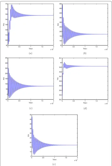
as-sumptionsS1andS2. From Theorem1, whenτ∈(0,τ0),E∗(147.6003, 170.9480, 77.8076,
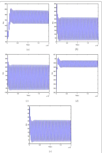
39.9170, 17.1176) is locally asymptotically stable, which can be illustrated in Figs. 2–3. While asτ is increased to passτ0, we can see the effect of time delay that destabilizes
system (21) and a Hopf bifurcation occurs and a periodic oscillation appears around E∗(147.6003, 170.9480, 77.8076, 39.9170, 17.1176). This can be shown as in Figs.4–5.
Figure 2The equilibriumE∗of system (21) is asymptotically stable forτ= 114.685 <τ0
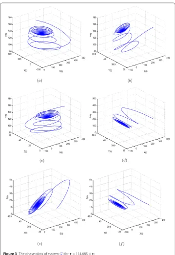
Figure 3The phase plots of system (2) forτ= 114.685 <τ0
5 Conclusions
Figure 4The equilibriumE∗of system (21) is unstable forτ= 122.905 >τ0
critical valueτ0, a Hopf bifurcation occurs and smoking will be out of control. Particularly,
properties such as direction and stability of the Hopf bifurcation are examined with the aid of the center manifold theorem and normal form theory.
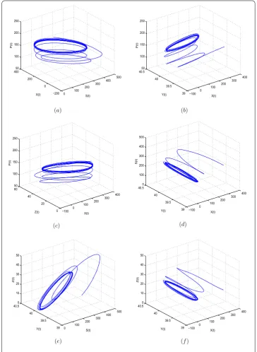
Figure 5The phase plots of system (2) forτ= 122.905 >τ0
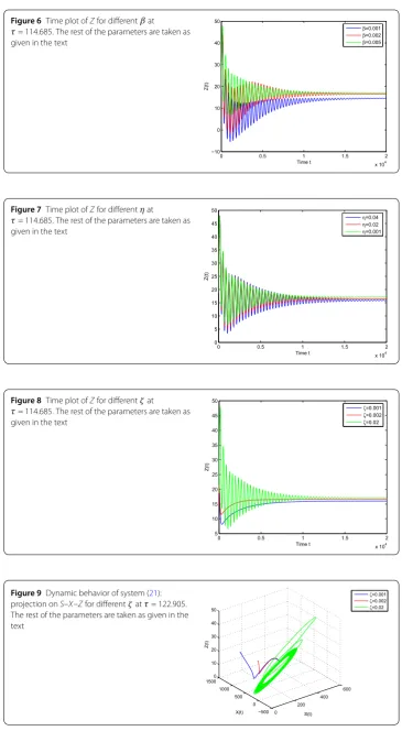
Figure 6Time plot ofZfor differentβat
τ= 114.685. The rest of the parameters are taken as given in the text
Figure 7Time plot ofZfor differentηat
τ= 114.685. The rest of the parameters are taken as given in the text
Figure 8Time plot ofZfor differentζat
τ= 114.685. The rest of the parameters are taken as given in the text
At last, it should be noted that similar to smoking addiction, the other public health problem is excessive drinking, which is not only harmful to personal health, but also leads to a range of negative social effects [35–37]. Therefore, we will try to complete some work about drink modeling in the near future.
Acknowledgements
The authors are very thankful to the anonymous reviewers for their insightful comments and suggestions, which helped us to improve the manuscript considerably and further open doors for future work.
Funding
This research was supported by the Project of Support Program for Excellent Youth Talent in Colleges and Universities of Anhui Province (No. gxyqZD2018044) and the Natural Science Foundation of the Higher Education Institutions of Anhui Province (Nos. KJ2019A0655, KJ2019A0656, KJ2019A0662).
Availability of data and materials
All of the authors declare that all the data can be accessed in our manuscript in the numerical simulation section.
Competing interests
The authors declare that there is no conflict of interests.
Authors’ contributions
All authors read and approved the final manuscript.
Publisher’s Note
Springer Nature remains neutral with regard to jurisdictional claims in published maps and institutional affiliations.
Received: 30 September 2019 Accepted: 3 December 2019
References
1. World Health Organization report on the global tobacco epidemic (2019). https://apps.who.int/iris/bitstream/handle/10665/326043/9789241516204-eng.pdf
2. Sun, C.X., Jia, J.W.: Optimal control of a delayed smoking model with immigration. J. Biol. Dyn.13, 447–460 (2019) 3. Khan, S.A., Shah, K., Zaman, G., Jarad, F.: Existence theory and numerical solutions to smoking model under
Caputo–Fabrizio fractional derivative. Chaos29, Article ID 013128 (2019).https://doi.org/10.1063/1.5079644 4. Rahman, G., Agarwal, R.P., Din, Q.: Mathematical analysis of giving up smoking model via harmonic mean type
incidence rate. Appl. Math. Comput.354, 128–148 (2019)
5. Garsow, C.C., Salivia, G.J., Herrera, A.R.: Mathematical models for dynamics of tobacco use, recovery and relapse. Technical report BU-1505-M, Cornell University, Ithaca, NY (2000)
6. Sharomi, O., Gumel, A.B.: Curtailing smoking dynamics: a mathematical modeling approach. Appl. Math. Comput. 195, 475–499 (2008)
7. Zaman, G.: Qualitative behavior of giving up smoking models. Bull. Malays. Math. Soc.34, 403–415 (2011) 8. Zeb, A., Zaman, G., Momani, S.: Square-root dynamics of a giving up smoking model. Appl. Math. Model.37,
5326–5334 (2013)
9. Huo, H.F., Zhu, C.C.: Influence of relapse in a giving up smoking model. Abstr. Appl. Anal.2013, Article ID 525461 (2013)
10. Bushnaq, S., Maayah, B., Alhabees, A.: Application of multistep reproducing kernel Hilbert space method for solving giving up smoking model. Int. J. Pure Appl. Math.109, 311–324 (2016)
11. Singh, J., Kumar, D., Qurashi, M.A., Baleanu, D.: A new fractional model for giving up smoking dynamics. Adv. Differ. Equ.2017, Article ID 88 (2017)
12. Haq, F., Shah, K., Rahman, G., Shahzad, M.: Numerical solution of fractional order smoking model via Laplace Adomian decomposition method. Alex. Eng. J.57, 1061–1069 (2018)
13. Labzai, A., Balatif, O., Rachik, M.: Optimal control strategy for a discrete time smoking model with specific saturated incidence rate. Discrete Dyn. Nat. Soc.2018, Article ID 5949303 (2018)
14. Rahman, G., Agarwal, R.P., Liu, L.L., Khan, A.: Threshold dynamics and optimal control of an age-structured giving up smoking model. Nonlinear Anal., Real World Appl.43, 96–120 (2018)
15. Fei, Y.L., Liu, X.D.: Spreading dynamic of a PLSGP giving up smoking model on scale-free network. Open Access Libr. J. 5, Article ID e4365 (2018)
16. Sharma, A., Misra, A.K.: Backward bifurcation in a smoking cessation model with media campaigns. Appl. Math. Model.39, 1087–1098 (2015)
17. Zhang, X.K., Zhang, Z.Z., Tong, J.Y., Dong, M.: Ergodicity of stochastic smoking model and parameter estimation. Adv. Differ. Equ.2016, Article ID 274 (2016)
18. Zaman, G., Kang, Y.H., Jung, I.H.: Dynamics of a smoking model with smoking death rate. Appl. Math.44, 281–295 (2017)
19. Pulecio-Montoya, A.M., Lopez-Montenegro, L.E., Benavides, L.M.: Analysis of a mathematical model of smoking. Contemp. Eng. Sci.12, 117–129 (2019)
20. Matintu, S.: Smoking as epidemic: modeling and simulation study. Am. J. Appl. Math.5, 31–38 (2017)
22. Wang, L.S., Xu, R., Feng, G.H.: Modelling and analysis of an eco-epidemiological model with time delay and stage structure. J. Appl. Math. Comput.50, 175–197 (2016)
23. Bai, Y.Z., Li, Y.Y.: Stability and Hopf bifurcation for a stage-structured predator–prey model incorporating refuge for prey and additional food for predator. Adv. Differ. Equ.2019, Article ID 42 (2019)
24. Xu, C.J.: Delay-induced oscillations in a competitor–competitor–mutualist Lotka–Volterra model. Complexity2017, Article ID 2578043 (2017)
25. Yuan, S.L., Song, Y.L.: Stability and Hopf bifurcations in a delayed Leslie–Gower predator–prey system. J. Math. Anal. Appl.355, 82–100 (2009)
26. Zhang, J.F.: Bifurcation analysis of a modified Holling–Tanner predator–prey model with time delay. Appl. Math. Model.36, 1219–1231 (2012)
27. Meng, X.Y., Wang, J.G.: Analysis of a delayed diffusive model with Beddington–Deangelis functional response. Int. J. Biomath.12, Article ID 1950047 (2019)
28. Kundu, S., Maitra, S.: Dynamics of a delayed predator–prey system with stage structure and cooperation for preys. Chaos Solitons Fractals114, 453–460 (2018)
29. Sun, X.G., Wei, J.J.: Stability and bifurcation analysis in a viral infection model with delays. Adv. Differ. Equ.2015, Article ID 332 (2015)
30. Keshri, N., Mishra, B.K.: Two time-delay dynamic model on the transmission of malicious signals in wireless sensor network. Chaos Solitons Fractals68, 151–158 (2014)
31. Hassard, B.D., Kazarinoff, N.D., Wan, Y.H.: Theory and Applications of Hopf Bifurcation. Cambridge University Press, Cambridge (1981)
32. Bianca, C., Ferrara, M., Guerrini, L.: The Cai model with time delay: existence of periodic solutions and asymptotic analysis. Appl. Math. Inf. Sci.7, 21–27 (2013)
33. Zhao, T., Bi, D.J.: Hopf bifurcation of a computer virus spreading model in the network with limited anti-virus ability. Adv. Differ. Equ.2017, Article ID 183 (2017)
34. Meng, X.Y., Huo, H.F., Zhang, X.B., Xiang, H.: Stability and Hopf bifurcation in a three species system with feedback delays. Nonlinear Dyn.64, 349–364 (2011)
35. Huo, H.F., Chen, Y.L., Xiang, H.: Stability of a binge drinking model with delay. J. Biol. Dyn.11, 210–225 (2017) 36. Xiang, H., Wang, Y., Huo, H.F.: Analysis of the binge drinking models with demographics and nonlinear infectivity on
networks. J. Appl. Anal. Comput.8, 1535–1554 (2018)